
Chapter 5: Indoor Scene Classification with TensorFlow Lite for Microcontrollers and the Arduino Nano
Computer vision is what made convolutional neural networks hugely popular. Without this deep learning algorithm, tasks such as object recognition, scene understanding, and pose estimation would be really challenging. Nowadays, many modern camera applications are powered by machine learning (ML), and we just need to take the smartphone to see them in action. Computer vision also finds space in microcontrollers, although with limitations given the reduced onboard memory.
In this chapter, we will see the benefit of adding sight to our tiny devices by recognizing indoor environments with the OV7670 camera module in conjunction with the Arduino Nano 33 BLE Sense board.
In the first part, we will learn how to acquire images from the OV7670 camera module. We will then focus on the model design, applying transfer learning with the Keras API to recognize kitchens and bathrooms. Finally, we will deploy the quantized TensorFlow Lite (TFLite) model on an Arduino Nano with the help of TensorFlow Lite for Microcontrollers (TFLu).
The goal of this chapter is to show how to apply transfer learning with TensorFlow and learn the best practices of using a camera module with a microcontroller.
In this chapter, we're going to implement the following recipes:
- Taking pictures with the OV7670 camera module
- Grabbing camera frames from the serial port with Python
- Converting QQVGA images from YCbCr422 to RGB888
- Building the dataset for indoor scene classification
- Applying transfer learning with Keras
- Preparing and testing the quantized TFLite model
- Reducing RAM usage by fusing crop, resize, rescale, and quantize
Technical requirements
To complete all the practical recipes of this chapter, we will need the following:
- An Arduino Nano 33 BLE Sense board
- A micro-USB cable
- 1 x half-size solderless breadboard
- 1 x OV7670 camera module
- 1 x push-button
- 18 x jumper wires (male to female)
- A laptop/PC with either Ubuntu 18.04+ or Windows 10 on x86-64
The source code and additional materials are available in Chapter05 (https://github.com/PacktPublishing/TinyML-Cookbook/tree/main/Chapter05).
Taking pictures with the OV7670 camera module
Adding sight to the Arduino Nano is our first step to unlocking computer vision applications.
In this first recipe, we will build an electronic circuit to take pictures from the OV7670 camera module using the Arduino Nano. Once we have assembled the circuit, we will use the Arduino pre-built CameraCaptureRawBytes sketch to transmit the pixel values over the serial.
The following Arduino sketch contains the code referred to in this recipe:
- 01_camera_capture.ino:
Getting ready
The OV7670 camera module is the main ingredient required in this recipe to take pictures with the Arduino Nano. It is one of the most affordable cameras for TinyML applications – you can buy it from various distributors for less than $10. Cost is not the only reason we went for this sensor, though. Other factors make this device our preferred option, such as the following:
- Frame resolution and color format support: Since microcontrollers have limited memory, we should consider cameras capable of transferring low-resolution images. The OV7670 camera unit is a good choice because it can output QVGA (320x240) and QQVGA (160x120) pictures. Furthermore, the device can encode the images in different color formats, such as RGB565, RGB444, and YUCbCr422.
- Software library support: Camera units can be complicated to control without a software driver. Therefore, vision sensors with software library support are generally recommended to make the programming straightforward. The OV7670 has a support library for the Arduino Nano 33 BLE Sense board (https://github.com/arduino-libraries/Arduino_OV767X), which is already integrated into the Arduino Web Editor.
These factors, along with voltage supply, power consumption, frame rate, and interface, are generally pondered when choosing a vision module for TinyML applications.
How to do it...
Let's start this recipe by taking a half breadboard with 30 rows and 10 columns and mounting the Arduino Nano vertically among the left and right terminal strips, as shown in the following figure:

Figure 5.1 – The Arduino Nano mounted vertically between the left and right terminal strips
The following steps will show how to assemble the circuit with the Arduino Nano, OV7670 module, and a push-button:
- Connect the OV7670 camera module to the Arduino Nano by using 16 male-to-female jumper wires, as illustrated in the following diagram:

Figure 5.2 – Wiring between the Arduino Nano and OV7670
Although the OV7670 has 18 pins, we only need to connect 16 of them.
The OV7670 camera module is connected to the Arduino Nano following the arrangement needed for the Arduino_OV767X support library.
Tip
You can find the pin arrangement required by the Arduino_OV767x support library at the following link:
https://github.com/arduino-libraries/Arduino_OV767X/blob/master/src/OV767X.h
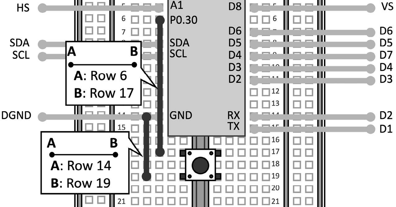
Figure 5.3 – Push-button connected between P0.30 and GND
The push-button does not need an additional resistor because we will employ the microcontroller pull-up one.
Now, open the Arduino IDE and follow these steps to implement a sketch to take pictures whenever we press the push-button:
- Open the CameraCaptureRawBytes sketch from Examples->FROM LIBRARIES->ARDUINO_OV767X:
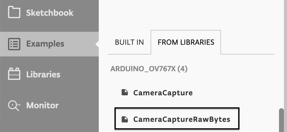
Figure 5.4 – CameraCaptureRawBytes sketch
Copy the content of CameraCaptureRawBytes in a new sketch.
- Declare and initialize a global mbed::DigitalIn object to read the push-button state:
mbed::DigitalIn button(p30);
#define PRESSED 0
Next, set the button mode to PullUp in the setup() function:
button.mode(PullUp);
- Set the baud rate of the serial peripheral to 115600 in the setup() function:
Serial.begin(115600);
- Add an if statement in the loop() function to check whether the push-button is pressed. If the button is pressed, take a picture from the OV7670 camera and send the pixel values over the serial:
if(button == PRESSED) {
Camera.readFrame(data);
Serial.write(data, bytes_per_frame);
}
Note
The variables' names in the pre-built CameraCaptureRawBytes are in PascalCase, so the first letter of each word is capitalized. To keep consistency with the lowercase naming convention used in the book, we have renamed BytesPerFrame to bytes_per_frame.
Compile and upload the sketch on the Arduino Nano. Now, you can open the serial monitor by clicking on Monitor from the Editor menu. From there, you will see all the pixels values transmitted whenever you press the push-button.
Grabbing camera frames from the serial port with Python
In the previous recipe, we showed how to take images from the OV7670, but we didn't present a method for displaying them.
This recipe will use Python to parse the pixel values transmitted serially to display the captured pictures on the screen.
The following Arduino sketch and Python script contain the code referred to in this recipe:
- 02_camera_capture_qvga_rgb565.ino:
- 02_parse_camera_frame.py:
Getting ready
In contrast to all Python programs developed so far, we will write the Python script on our local machine to access the serial port used by the Arduino Nano.
Parsing serial data with Python requires little effort with the pySerial library, which can be installed through the pip Python package manager:
$ pip install pyserial
However, pySerial will not be the only module required for this recipe. Since we need to create images from the data transmitted over the serial, we will use the Python Pillow library (PIL) to facilitate this task.
The PIL module can be installed with the following pip command:
$ pip install Pillow
However, what data format should we expect from the microcontroller?
Transmitting RGB888 images over the serial
To simplify the parsing of the pixels transmitted over the serial, we will make some changes in the Arduino sketch of the previous recipe to send images in RGB888 format. This format packs the pixel in 3 bytes, using 8 bits for each color component.
Using RGB888 means that our Python script can directly create the image with PIL without extra conversions.
However, it is a good practice to transmit the image with metadata to simplify the parsing and check communication errors.
In our case, the metadata will provide the following information:
- The beginning of the image transmission: We send the <image> string to signify the beginning of the communication.
- The image resolution: We send the image resolution as a string of digits to say how many RGB pixels will be transmitted. The width and height will be sent on two different lines.
- The completion of the image transmission: Once we have sent all pixel values, we transmit the </image> string to notify the end of the communication.
The pixel values will be sent right after the image resolution metadata and following the top to bottom, left to right order (raster scan order):
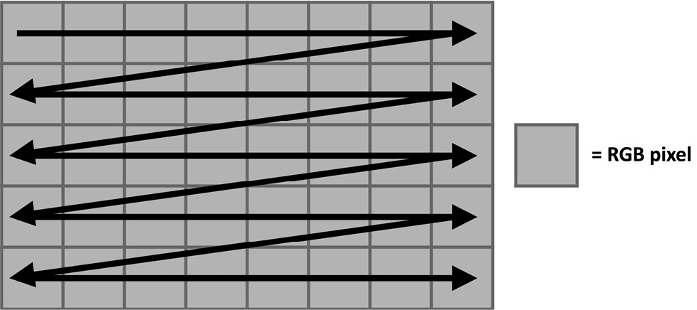
Figure 5.5 – Raster scan order
The color components will be sent as strings of digits terminated with a newline character ( ) and following the RGB ordering. Therefore, the red channel comes first and the blue one last, as shown in the following diagram:
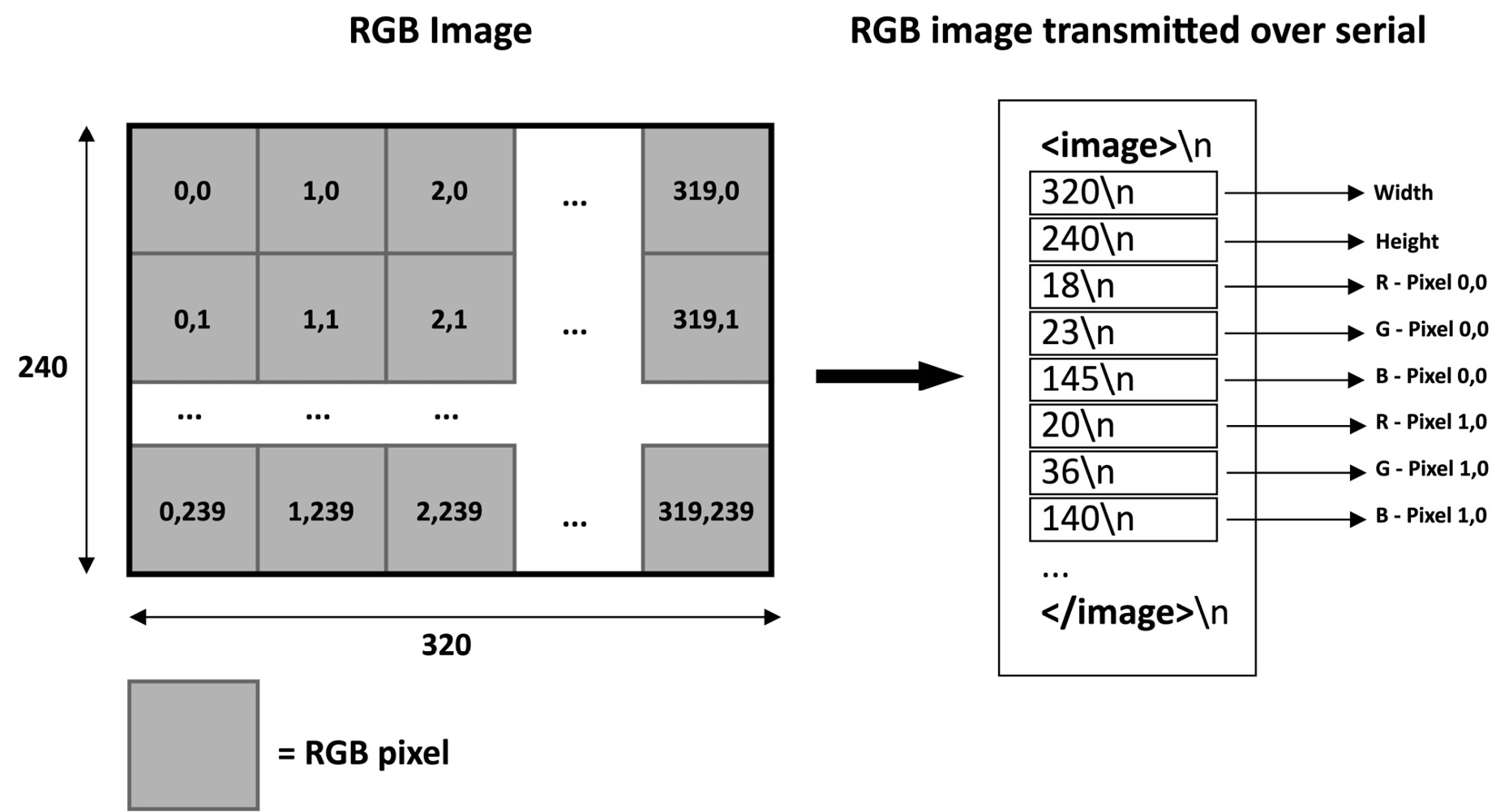
Figure 5.6 – Communication protocol for the serial transmission of an RGB image
As you can observe from the preceding illustration, the pixel values are transmitted following the raster scanning order. Each color component is sent as a string of digits terminated with a newline character ( ).
However, the OV7670 camera is initialized to output images in the RGB565 color format. Therefore, we need to convert the camera pixels to RGB888 before sending them over the serial.
Learning how to convert RGB565 to RGB888
As you may have noticed, RGB565 is the format used in the camera initialization of the CameraCaptureRawBytes sketch:
Camera.begin(QVGA, RGB565, 1)
RGB565 packs the pixel in 2 bytes, reserving 5 bits for the red and blue components and 6 bits for the green one:
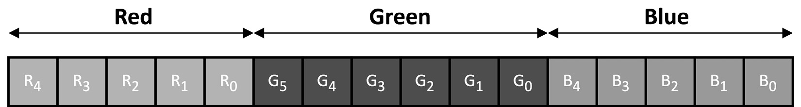
Figure 5.7 – RGB565 color format
This color format finds applicability mainly in embedded systems with limited memory capacity since it reduces the image size. However, memory reduction is achieved by reducing the dynamic range of the color components.
How to do it...
In the following steps, we will see what to change in the Arduino sketch of the previous recipe to send the RGB888 pixels over the serial. Once the sketch is implemented, we will write a Python script to display the image transmitted over the serial on the screen:
- Write a function to convert the RGB565 pixel to RGB888:
void rgb565_rgb888(uint8_t* in, uint8_t* out) {
uint16_t p = (in[0] << 8) | in[1];
out[0] = ((p >> 11) & 0x1f) << 3;
out[1] = ((p >> 5) & 0x3f) << 2;
out[2] = (p & 0x1f) << 3;
}
The function takes 2 bytes from the input buffer to form the 16-bit RGB565 pixel. The first byte (in[0]) is left-shifted by eight positions to place it in the higher half of the uint16_t p variable. The second byte (in[1]) is set in the lower part:
![Figure 5.8 – The RGB565 pixel is formed with in[0] and in[1] bytes](https://imgdetail.ebookreading.net/2023/10/9781801814973/9781801814973__9781801814973__files__image__B17710_05_08.jpg)
Figure 5.8 – The RGB565 pixel is formed with in[0] and in[1] bytes
Once we have the 16-bit pixel, we get the 8-bit color components from p by right-shifting each channel towards the beginning of the least significant byte:
- The 8-bit red channel (out[0]) is obtained by shifting p by 11 positions so that R0 is the first bit of the uint16_t variable. After, we clear all the non-red bits by applying a bitmask with 0x1F (all bits cleared except the first five).
- The 8-bit green channel (out[1]) is obtained by shifting p by five positions so that G0 is the first bit of the uint16_t variable. After, we clear all the non-green bits by applying a bitmask with 0x3F (all bits cleared except the first six).
- The 8-bit blue channel (out[2]) is obtained without shifting because B0 is already the first bit of the uint16_t variable. Therefore, we just need to clear the non-blue bits by applying a bitmask with 0x1F (all bits cleared except the first five).
In the end, we perform an extra left-shifting to move the most significant bit of each channel to the eighth position of the byte.
- Enable testPattern in the setup() function:
Camera.testPattern();
The Camera module will always return a fixed image with color bands when the test pattern mode is enabled.
- In the loop() function, replace Serial.write(data, bytes_per_frame) with the routine to send the RGB888 pixels over the serial:
Camera.readFrame(data);
uint8_t rgb888[3];
Serial.println("<image>");
Serial.println(Camera.width());
Serial.println(Camera.height());
const int bytes_per_pixel = Camera.bytesPerPixel();
for(int i = 0; i < bytes_per_frame; i+=bytes_per_pixel) {
rgb565_rgb888(&data[i], &rgb888[0]);
Serial.println(rgb888[0]);
Serial.println(rgb888[1]);
Serial.println(rgb888[2]);
}
Serial.println("</image>");
The communication starts by sending the <image> string and the resolution of the image (Camera.width(), Camera.height()) over the serial.
Next, we iterate all bytes stored in the camera buffer and apply the RGB565 to RGB888 conversion with the rgb565_rgb888() function. Every color component is then sent as a string of digits with the newline character ( ).
When we complete the conversion, we send the </image> string to signify the end of the data transmission.
Now, you can compile and upload the sketch on the Arduino Nano.
- On your computer, create a new Python script and import the following modules:
import numpy as np
import serial
from PIL import Image
- Initialize pySerial with the port and baud rate used by the Arduino Nano's microcontroller:
port = '/dev/ttyACM0'
baudrate = 115600
ser = serial.Serial()
ser.port = port
ser.baudrate = baudrate
The easiest way to check the serial port name is from the device drop-down menu in the Arduino IDE:

Figure 5.9 – Device drop-down menu in the Arduino Web Editor
In the preceding screenshot, the serial port name is /dev/ttyACM0.
Then, open the serial port and discard the content in the input buffer:
ser.open()
ser.reset_input_buffer()
- Create a utility function to return a line from the serial port as a string:
def serial_readline():
data = ser.readline
return data.decode("utf-8").strip()
The string transmitted by the Arduino Nano over the serial is encoded in UTF-8 and terminates with the newline character. Therefore, we decode the UTF-8 encoded bytes and remove the newline character with .decode("utf-8") and .strip().
- Create a 3D NumPy array to store the pixel values transmitted over the serial. Since the Arduino Nano will send the frame resolution, you can initialize the width and height with 1 and resize the NumPy array later when parsing the serial stream:
width = 1
height = 1
num_ch = 3
image = np.empty((height, width, num_ch), dtype=np.uint8)
- Use a while loop to read the serial data line by line:
while True:
data_str = serial_readline()
Check whether we have the <image> metadata:
if str(data_str) == "<image>":
If so, parse the frame resolution (width and height) and resize the NumPy array accordingly:
w_str = serial_readline()
h_str = serial_readline()
w = int(w_str)
h = int(h_str)
if w != width or h != height:
if w * h != width * height:
image.resize((h, w, num_ch))
else:
image.reshape((h, w, num_ch))
width = w
height = h
- Once you know the frame resolution, parse the pixel values transmitted over the serial, and store them in the NumPy array:
for y in range(0, height):
for x in range(0, width):
for c in range(0, num_ch):
data_str = serial_readline()
image[y][x][c] = int(data_str)
To have a more efficient solution, you may consider the following alternative code without nested for loops:
for i in range(0, width * height * num_ch):
c = int(i % num_ch)
x = int((i / num_ch) % width)
y = int((i / num_ch) / width)
data_str = serial_readline()
image[y][x][c] = int(data_str)
- Check if the last line contains the </image> metadata. If so, display the image on the screen:
data_str = serial_readline()
if str(data_str) == "</image>":
image_pil = Image.fromarray(image)
image_pil.show()
Keep the Arduino Nano connected to your machine and run the Python script. Now, whenever you press the push-button, the Python program will parse the data transmitted over the serial and, after a few seconds, show an image with eight color bands, as reported at the following link:
https://github.com/PacktPublishing/TinyML-Cookbook/blob/main/Chapter05/test_qvga_rgb565.png
If you do not get the image with the test pattern just described, we recommend checking the wiring between the camera and the Arduino Nano.
Converting QQVGA images from YCbCr422 to RGB888
When compiling the previous sketch on Arduino, you may have noticed the Low memory available, stability may occur warning in the Arduino IDE output log.
The Arduino IDE returns this warning because the QVGA image with the RGB565 color format needs a buffer of 153.6 KB, which is roughly 60% of the SRAM available in the microcontroller.
In this recipe, we will show how to acquire an image at a lower resolution and use the YCbCr422 color format to prevent image quality degradation.
The following Arduino sketch contains the code referred to in this recipe:
- 03_camera_capture_qqvga_ycbcr422.ino:
Getting ready
The main ingredients to reduce the image size are behind the resolution and color format.
Images are well known for requiring big chunks of memory, which might be a problem when dealing with microcontrollers.
Lowering the image resolution is a common practice to reduce the image memory size.Standard resolution images adopted on microcontrollers are generally smaller than QVGA (320x240), such as QQVGA (160x120) or QQQVGA (80x60). Even lower-resolution images exist, but they are not always suitable for computer vision applications.
Color encoding is the other lever to reduce the image memory size. As we saw in the previous recipe, the RGB565 format saves memory by lowering the color components' dynamic range. However, the OV7670 camera module offers an alternative and more efficient color encoding: YCbCr422.
Converting YCbCr422 to RGB888
YCbCr422 is digital color encoding that does not express the pixel color in terms of red, green, and blue intensities but rather in terms of brightness (Y), blue-difference (Cb), and red-difference (Cr) chroma components.
The OV7670 camera module can output images in YCbCr422 format, which means that Cb and Cr are shared between two consecutive pixels on the same scanline. Therefore, 4 bytes are used to encode 2 pixels:

Figure 5.10 – 4 bytes in YCbCr422 format packs 2 RGB888 pixels
Although YCbCr422 still needs 2 bytes per pixel as RGB565, it offers better image quality.
The following table reports the formulas to accomplish the color conversion from YCbCr422 to RGB888 using just integer arithmetic operations:

Figure 5.11 – Table reporting the formulas to convert YCbCr422 to RGB888
The i subscript in Ri, Gi, Bi, and Yi represents the pixel index, either 0 (the first pixel) or 1 (the second pixel).
How to do it...
Open the Arduino sketch written in the previous recipe and make the following changes to acquire QQVGA YCbCr422 images from the OV7670 camera module:
- Resize the camera buffer (data) to accommodate a QQVGA image in YCbCr422 color format:
byte data[160 * 120 * 2];
The QQVGA resolution makes the buffer four times smaller than the one used in the previous recipe.
- Write a function to get an RGB888 pixel from the Y, Cb, and Cr components:
template <typename T>
inline T clamp_0_255(T x) {
return std::max(std::min(x, (T)255)), (T)(0));
}
void ycbcr422_rgb888(int32_t Y, int32_t Cb,
int32_t Cr, uint8_t* out) {
Cr = Cr - 128;
Cb = Cb - 128;
out[0] = clamp_0_255((int)(Y + Cr + (Cr >> 2) +
(Cr >> 3) + (Cr >> 5)));
out[1] = clamp_0_255((int)(Y - ((Cb >> 2) + (Cb >> 4) +
(Cb >> 5)) - ((Cr >> 1) +
(Cr >> 3) + (Cr >> 4)) +
(Cr >> 5)));
out[2] = clamp_0_255((int)(Y + Cb + (Cb >> 1) +
(Cb >> 2) + (Cb >> 6)));
}
The function returns two pixels because the Cb and Cr components are shared between two pixels.
The conversion is performed using the formulas provided in the Getting ready section.
Attention
Please note that the OV7670 driver returns the Cr component before the Cb one.
- Initialize the OV7670 camera to capture QQVGA frames with YCbCr422 (YUV422) color format in the setup() function:
if (!Camera.begin(QQVGA, YUV422, 1)) {
Serial.println("Failed to initialize camera!");
while (1);
}
Unfortunately, the OV7670 driver interchanges YCbCr422 with YUV422, leading to some confusion. The main difference between YUV and YCbCr is that YUV is for analog TV. Therefore, although we pass YUV422 to Camera.begin(), we actually initialize the device for YCbCr422.
- In the loop() function, remove the statement that iterates over the RGB565 pixels stored in the previous camera buffer. Next, write a routine to read 4 bytes from the YCbCr422 camera buffer and return two RGB888 pixels:
const int step_bytes = Camera.bytesPerPixel() * 2;
for(int i = 0; i < bytes_per_frame; i+=step_bytes) {
const int32_t Y0 = data[i + 0];
const int32_t Cr = data[i + 1];
const int32_t Y1 = data[i + 2];
const int32_t Cb = data[i + 3];
ycbcr422_to_rgb888_i(Y0, Cb, Cr, &rgb888[0]);
Serial.println(rgb888[0]);
Serial.println(rgb888[1]);
Serial.println(rgb888[2]);
ycbcr422_to_rgb888_i(Y1, Cb, Cr, &rgb888[0]);
Serial.println(rgb888[0]);
Serial.println(rgb888[1]);
Serial.println(rgb888[2]);
}
Compile and upload the sketch on the Arduino Nano. Execute the Python script and press the push-button on the breadboard. After a few seconds, you should see on the screen, again, an image with eight color bands, as reported at the following link: https://github.com/PacktPublishing/TinyML-Cookbook/blob/main/Chapter05/test_qqvga_ycbcr422.png.
The image should be smaller but with more vivid colors than the one captured with the RGB565 format.
Building the dataset for indoor scene classification
Now that we can capture frames from the camera, it is time to create the dataset for classifying indoor environments.
In this recipe, we will construct the dataset by collecting the kitchen and bathroom images with the OV7670 camera.
The following Python script contains the code referred to in this recipe:
- 04_build_dataset.py:
Getting ready
Training a deep neural network from scratch for image classification commonly requires a dataset with 1,000 images per class. As you might guess, this solution is impractical for us since collecting thousands of pictures takes a lot of time.
Therefore, we will consider an alternative ML technique: transfer learning.
Transfer learning is a popular method that uses a pre-trained model to train a deep neural network with a small dataset. This ML technique will be used in the following recipe and only requires a dataset with just 20 samples per class to get a basic working model.
How to do it...
Before implementing the Python script, remove the test pattern mode (Camera.testPattern()) in the Arduino sketch so that you can get live images. After that, compile and upload the sketch on the platform.
The Python script implemented in this recipe will reuse part of the code developed in the earlier Grabbing camera frames from the serial port with Python recipe. The following steps will show what changes to make in the Python script to save the captured images as .png files and build a dataset for recognizing kitchens and bathrooms:
- Import the UUID Python module:
import uuid
UUID will be used to produce unique filenames for .png files.
- Add a variable at the beginning of the program for the label's name:
label = "test"
The label will be the prefix for the filename of the .png files.
- After receiving the image over the serial, crop it into a square shape and display it on the screen:
crop_area = (0, 0, height, height)
image_pil = Image.fromarray(image)
image_cropped = image_pil.crop(crop_area)
image_cropped.show()
We crop the acquired image from the serial port into a square shape because the pre-trained model will consume an input with a square aspect ratio. We crop the left side of the image by taking an area with dimensions matching the height of the original picture, as shown in the following figure:

Figure 5.12 – Cropping area
The picture is then displayed on the screen.
- Ask the user if the image can be saved and read the response with the Python input() function. If the user types y from the keyboard, ask for the label's name and save the image as a .png file:
key = input("Save image? [y] for YES: ")
if key == 'y':
str_label = "Write label or leave it blank to use [{}]: ".format(label)
label_new = input(str_label)
if label_new != '':
label = label_new
unique_id = str(uuid.uuid4())
filename = label + "_"+ unique_id + ".png"
image_cropped.save(filename)
If the user leaves the label empty, the program will use the last label provided.
The filename for the .png file is <label>_<unique_id>, where <label> is the label chosen by the user and <unique_id> is the unique identifier generated by the UUID library.
- Acquire 20 images of kitchens and the bathrooms with the OV7670 camera. Since we only take a few pictures per class, we recommend you point the camera to specific elements of the rooms.
Remember to take 20 pictures for the unknown class as well, representing cases where we have neither a kitchen nor a bathroom.
Once you have acquired all the images, put them in separate subdirectories, matching the name of the corresponding class, as shown in the following directory structure:
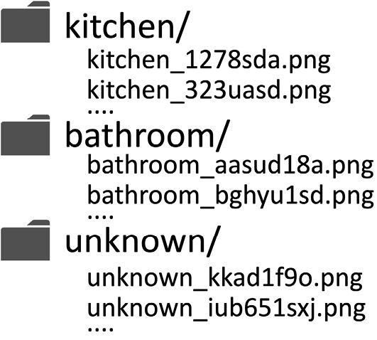
Figure 5.13 – Example of a directory structure
In the end, generate a .zip file with the three folders.
Transfer learning with Keras
Transfer learning is an effective technique for getting immediate results with deep learning when dealing with small datasets.
In this recipe, we will apply transfer learning alongside the MobileNet v2 pre-trained model to recognize indoor environments.
The following Colab notebook (the Transfer learning with Keras section) contains the code referred to in this recipe:
- prepare_model.ipynb:
Getting ready
Transfer learning exploits a pre-trained model to obtain a working ML model in a short time.
When doing image classification with transfer learning, the pre-trained model (convolution based network) is coupled with a trainable classifier (head), as shown in the following figure:

Figure 5.14 – Model architecture with transfer learning
As you can observe from the previous illustration, the pre-trained model is the backbone of feature extraction and feeds the classifier, commonly made of global pooling, dense, and softmax layers.
In our scenario, we will only train the classifier. Hence, the pre-trained model will be frozen and act as a fixed feature extractor.
Keras provides different pre-trained models, such as VGG16, ResNet50, InceptionV3, MobileNet, and so on. Therefore, which one should we use?
When considering a pre-trained model for TinyML, model size is the metric to keep in mind to fit the deep learning architecture into memory-constrained devices.
From the list of pre-trained models offered by Keras (https://keras.io/api/applications/), MobileNet v2 is the network with fewer parameters and tailored for being deployed on target devices with reduced computational power.
Exploring the MobileNet network design choices
MobileNet v2 is the second generation of MobileNet networks and, compared to the previous one (MobileNet v1), it has half as many operations and higher accuracy.
This model is the perfect place to take a cue from the architectural choices that made MobileNet networks small, fast, and accurate for edge inferencing.
One of the successful design choices that made the first generation of MobileNet networks suitable for edge inferencing was the adoption of depthwise convolution.
As we know, traditional convolution layers are well known for being computationally expensive. Furthermore, when dealing with 3x3 or greater kernel sizes, this operator typically needs extra temporary memory to lower the computation to a matrix multiplication routine.
The idea behind MobileNet v1 was to replace standard convolution 2D with depthwise separable convolution, as shown in the following diagram:
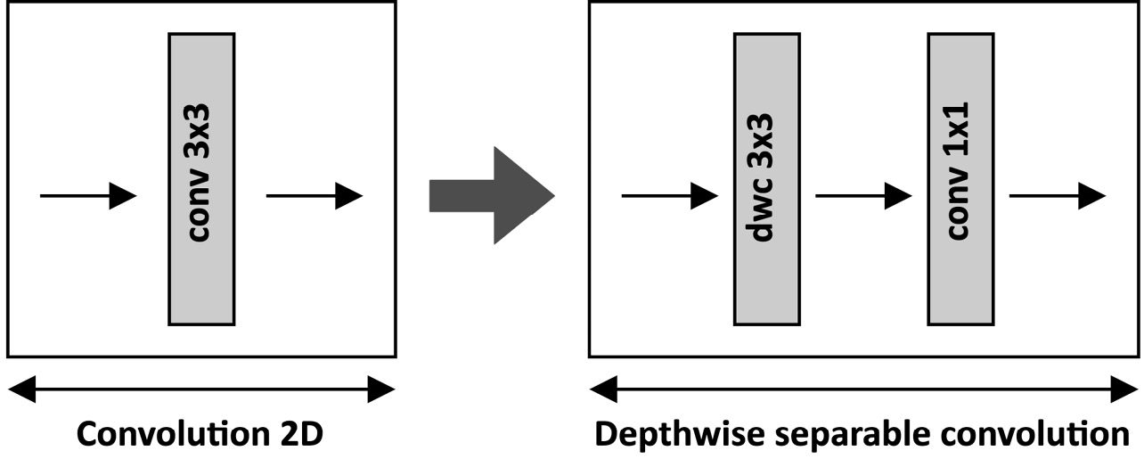
Figure 5.15 – Depthwise separable convolution
As you can observe from the preceding illustration, depthwise separable convolution consists of a depthwise convolution with a 3x3 filter size followed by a convolution layer with a 1x1 kernel size (also known as pointwise convolution). This solution brings less trainable parameters, less memory usage, and a lower computational cost.
Tip
Chapter 7, Running a Tiny CIFAR-10 Model on a Virtual Platform with the Zephyr OS will provide more information on the benefits given by depthwise separable convolution.
The computational cost on MobileNet v2 was reduced further by performing the convolutions on tensors with fewer channels.
From an ideal computational perspective, all the layers should work on tensors with few channels (feature maps) to improve the model latency. Practically, and from an accuracy perspective, it means that our compact tensors can keep the relevant features for the problem we want to solve.
Depthwise separable convolution alone cannot help because a reduction in the number of feature maps causes a drop in the model accuracy. Therefore, MobileNet v2 introduced the bottleneck residual block to keep the number of channels used in the network smaller:

Figure 5.16 – Bottleneck residual block
The bottleneck residual block acts as a feature compressor. As illustrated in the preceding diagram, the input is processed by the pointwise convolution, which expands (or increases) the number of features maps. Then, the convolution's output feeds the depthwise separable convolution layer to compress the features in fewer output channels.
How to do it...
Create a new Colab notebook. Next, upload the .zip file containing the dataset (dataset.zip) by using the upload button at the top of the file explorer:

Figure 5.17 – Upload button at the top of the file explorer
Now, follow these steps to apply transfer learning with the MobileNet v2 pre-trained model:
- Unzip the dataset:
import zipfile
with zipfile.ZipFile("dataset.zip", 'r') as zip_ref:
zip_ref.extractall(".")
data_dir = "dataset"
- Prepare the training and validation datasets:
train_ds = tf.keras.utils.image_dataset_from_directory(
data_dir,
validation_split=0.2,
subset="training",
seed=123,
interpolation="bilinear",
image_size=(48, 48))
val_ds = tf.keras.utils.image_dataset_from_directory(
data_dir,
validation_split=0.2,
subset="validation",
seed=123,
interpolation="bilinear",
image_size=(48, 48))
- The preceding code resizes the input images to 48x48 with the bilinear interpolation and produces the training and validation datasets with an 80/20 split.
- Rescale the pixel values from [0, 255] to [-1, 1]:
rescale = tf.keras.layers.Rescaling(1./255, offset= -1)
train_ds = train_ds.map(lambda x, y: (rescale(x), y))
val_ds = val_ds.map(lambda x, y: (rescale(x), y))
The reason for rescaling the pixels values from [0, 255] to [-1, 1] is because the pre-trained model expects this interval data range for the input tensor.
- Import the MobileNet v2 pre-trained model with the weights trained on the ImageNet dataset and alpha=0.35. Furthermore, set the input image at the lowest resolution allowed by the pre-trained model (48, 48, 3) and exclude the top (fully-connected) layers:
base_model = MobileNetV2(input_shape=(48, 48, 3),
include_top=False,
weights='imagenet',
alpha=0.35)
Keras offers more than one variant of MobileNet v2. From the list of MobileNet v2 Keras models (https://github.com/keras-team/keras-applications/blob/master/keras_applications/mobilenet_v2.py), we choose mobilenet_v2_0.35_96, which has the smallest input size (48,48,3) and the smallest alpha value (0.35).
- Freeze the weights so that you do not update these values during training:
base_model.trainable = False
feat_extr = base_model
- Augment the input data:
augmen = tf.keras.Sequential([
tf.keras.layers.experimental.preprocessing.RandomFlip('horizontal'), tf.keras.layers.experimental.preprocessing.RandomRotation(0.2),])
train_ds = train_ds.map(lambda x, y: (augmen(x), y))
val_ds = val_ds.map(lambda x, y: (augmen(x), y))
Since we don't have a large dataset, we recommend artificially applying some random transformations on the images to prevent overfitting.
- Prepare the classification head with a global pooling followed by a dense layer with a softmax activation:
global_avg_layer = tf.keras.layers.GlobalAveragePooling2D()
dense_layer = tf.keras.layers.Dense(3,
activation='softmax')
- Build the model architecture:
inputs = tf.keras.Input(shape=MODEL_INPUT_SIZE)
x = global_avg_layer(feat_extr.layers[-1].output)
x = tf.keras.layers.Dropout(0.2)(x)
outputs = dense_layer(x)
model = tf.keras.Model(inputs=feat_extr.inputs,
outputs=outputs)
We recommend passing training=False to the feature extractor module to not update the batch normalization layers' internal variables (mean and variance) in MobileNet v2.
- Compile the model with a 0.0005 learning rate:
lr = 0.0005
model.compile(
optimizer=tf.keras.optimizers.Adam(learning_rate=lr),
loss=tf.losses.SparseCategoricalCrossentropy(from_logits=False),
metrics=['accuracy'])
The default learning rate used by TensorFlow is 0.001. The reason for reducing the learning rate to 0.0005 is to prevent overfitting.
- Train the model with 10 epochs:
model.fit(
train_ds,
validation_data=val_ds,
epochs=10)
The expected accuracy on the validation dataset should be around 90% or more.
- Save the TensorFlow model as SavedModel:
model.save("indoor_scene_recognition")
The model is now ready to be quantized with the TFLite converter.
Preparing and testing the quantized TFLite model
As we know from Chapter 3, Building a Weather Station with TensorFlow Lite for Microcontrollers, the model requires quantization to 8 bits to run more efficiently on a microcontroller. However, how do we know if the model can fit into the Arduino Nano? Furthermore, how do we know if the quantized model preserves the accuracy of the floating-point variant?
These questions will be answered in this recipe, where we will show how to evaluate the program memory utilization and the accuracy of the quantized model generated by the TFLite converter. After analyzing the memory usage and accuracy validation, we will convert the TFLite model to a C-byte array.
The following Colab notebook (the Preparing and testing the quantized TFLite model section) contains the code referred to in this recipe:
- prepare_model.ipynb:
Getting ready
The model's memory requirement and accuracy evaluation should always be done to avoid unpleasant surprises when deploying the model on the target device. For example, the C-byte array generated from the TFLite model is typically a constant object stored in the microcontroller program memory. However, the program memory has a limited capacity, and usually, it does not exceed 1 MB.
The memory requirement is not the only problem we may encounter, though. Quantization is an effective technique to reduce the model size and significantly improve latency. However, the adoption of arithmetic with limited precision may change the model's accuracy. For this reason, it is crucial to assess the accuracy of the quantized model to be sure that the application works as expected. Unfortunately, TFLite does not provide a built-in function to evaluate the accuracy of the test dataset. Hence, we will need to run the quantized TFLite model through the Python TFLite interpreter over the test samples to check how many are correctly classified.
How to do it...
Let's start by collecting some test samples with the OV7670 camera module. You can follow the same steps presented in the early Building the dataset for indoor scene classification recipe. You just need to take a few pictures (for example, 10) for each output class and create a .zip file (test_samples.zip) with the same folder structure we had for the training dataset.
Next, upload the .zip file in Colab and follow the following steps to evaluate the accuracy of the quantized model and examine the model size:
- Unzip the test_samples.zip file:
with zipfile.ZipFile("test_samples.zip", 'r') as zip_ref:
zip_ref.extractall(".")
test_dir = "test_samples"
- Resize the test images to 48x48 with bilinear interpolation:
test_ds = tf.keras.utils.image_dataset_from_directory(
test_dir,
interpolation="bilinear",
image_size=(48, 48))
- Rescale the pixels values from [0, 255] to [-1, 1]:
test_ds = test_ds.map(lambda x, y: (rescale(x), y))
- Convert the TensorFlow model to TensorFlow Lite format (FlatBuffers) with the TensorFlow Lite converter tool. Apply the 8-bit quantization to the entire model except for the output layer:
repr_ds = test_ds.unbatch()
def representative_data_gen():
for i_value, o_value in repr_ds.batch(1).take(60):
yield [i_value]
TF_MODEL = "indoor_scene_recognition"
converter = tf.lite.TFLiteConverter.from_saved_model(TF_MODEL)
converter.representative_dataset = tf.lite.RepresentativeDataset(representative_data_gen)
converter.optimizations = [tf.lite.Optimize.DEFAULT]
converter.target_spec.supported_ops = [tf.lite.OpsSet.TFLITE_BUILTINS_INT8]
converter.inference_input_type = tf.int8
tfl_model = converter.convert()
The conversion is done in the same way we did it in Chapter 3, Building a Weather Station with TensorFlow Lite for Microcontrollers, except for the output data type. In this case, the output is kept in floating-point format to avoid the dequantization of the output result.
- Get the TFLite model size in bytes:
print(len(tfl_model), "bytes")
The generated TFLite object (tfl_model) is what we deploy on the microcontroller, which contains the model architecture and the weights of the trainable layers. Since the weights are constant, the TFLite model can be stored in the microcontroller program memory, and the length of the tfl_model object provides its memory usage. The expected model size is 627880, roughly 63% of the total program memory.
- Initialize the TFLite interpreter:
interpreter = tf.lite.Interpreter(model_content=tfl_model)
interpreter.allocate_tensors()
Unfortunately, TFLite does not offer pre-built functions to evaluate the model accuracy as the TensorFlow counterpart. Therefore, we require running the quantized TensorFlow Lite model in Python to evaluate the accuracy of the test dataset. The Python TFLite interpreter is responsible for loading and executing the TFLite model.
- Get the input quantization parameters:
i_details = interpreter.get_input_details()[0]
o_details = interpreter.get_output_details()[0]
i_quant = i_details["quantization_parameters"]
i_scale = i_quant['scales'][0]
i_zero_point = i_quant['zero_points'][0]
- Evaluate the accuracy of the quantized TFLite model:
test_ds0 = test_ds.unbatch()
num_correct_samples = 0
num_total_samples = len(list(test_ds0.batch(1)))
for i_value, o_value in test_ds0.batch(1):
i_value = (i_value / i_scale) + i_zero_point
i_value = tf.cast(i_value, dtype=tf.int8)
interpreter.set_tensor(i_details["index"], i_value)
interpreter.invoke()
o_pred = interpreter.get_tensor(o_details["index"])[0]
if np.argmax(o_pred) == o_value:
num_correct_samples += 1
print("Accuracy:", num_correct_samples/num_total_samples)
- Convert the TFLite model to a C-byte array with xxd:
open("model.tflite", "wb").write(tflite_model)
!apt-get update && apt-get -qq install xxd
!xxd -c 60 -i model.tflite > indoor_scene_recognition.h
The command generates a C header file containing the TensorFlow Lite model as an unsigned char array. Since the Arduino Web Editor truncates C files exceeding 20,000 lines, we recommend passing the -c 60 option to xxd. This option increases the number of columns per line from 16 (the default) to 60 to have roughly 10,500 lines in the file.
You can now download the indoor_scene_recognition.h file from Colab's left pane.
Reducing RAM usage by fusing crop, resize, rescale, and quantize
In this last recipe, we will deploy the application on the Arduino Nano. However, a few extra operators are needed to recognize indoor environments with our tiny device.
In this recipe, we will learn how to fuse crop, resize, rescale, and quantize operators to reduce RAM usage. These extra operators will be needed to prepare the TFLite model's input.
The following Arduino sketch contains the code referred to in this recipe:
- 07_indoor_scene_recognition.ino:
Getting ready
To get ready for this recipe, we need to know what parts of the application affect RAM usage.
RAM usage is impacted by the variables allocated during the program execution, such as the input, output, and intermediate tensors of the ML model. However, the model is not solely responsible for memory utilization. In fact, the image acquired from the OV7670 camera needs to be processed with the following operations to provide the appropriate input to the model:
- Convert the color format from YCbCr422 to RGB888.
- Crop the camera frame to match the input shape aspect ratio of the TFLite model.
- Resize the camera frame to match the expected input shape of the TFLite model.
- Rescale the pixel values from [0, 255] to [-1, 1].
- Quantize the floating-point pixel values.
Each of the preceding operations reads values from a buffer and returns the computation result in a new one, as shown in the following figure:
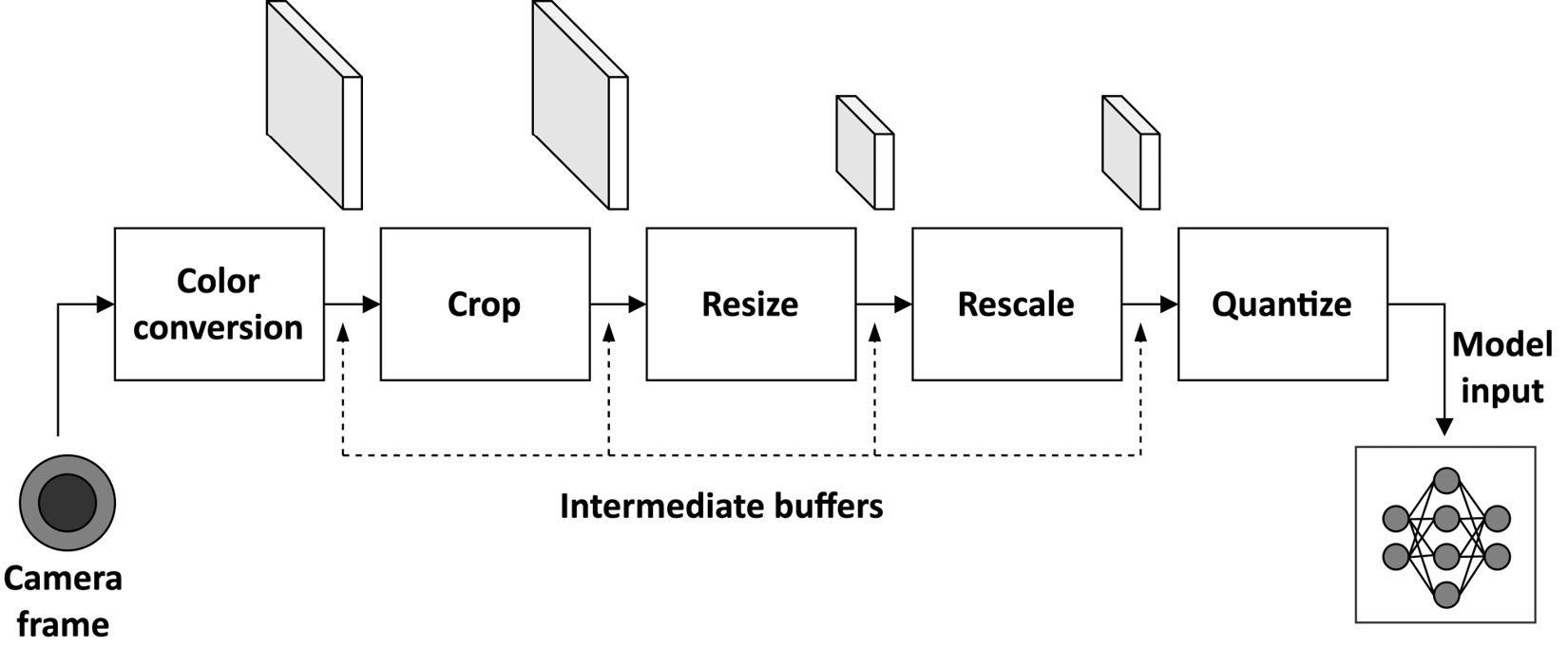
Figure 5.18 – Input preparation pipeline
Therefore, RAM usage is also affected by the camera frame and intermediate buffers passed from one operation to the next.
Our goal is to execute the processing pipeline described previously using as small intermediate buffers as possible.
To achieve this goal, the data propagated throughout the pipeline must represent a portion of the entire input to be processed. By adopting this technique, commonly called operator fusion, the camera frame will be the only considerable chunk of memory to reside in RAM in addition to the input, output, and intermediate tensors of the TFLite model.
Before showing how to implement this final recipe, let's see how to implement resizing in more detail.
Resizing with bilinear interpolation
Resizing is an image processing function used to alter the image's resolution (width and height), as shown in the following figure:

Figure 5.19 – Resize operation
The resulting image is created from the pixels of the input image. Generally, the following formulas are applied to map the spatial coordinates of the output pixels with the corresponding input ones:


From the previous two formulas, (![]() ) are the spatial coordinates of the input pixel, (
) are the spatial coordinates of the input pixel, (![]() ) are the spatial coordinates of the output pixel, (
) are the spatial coordinates of the output pixel, (![]() ) are the dimensions of the input image, and (
) are the dimensions of the input image, and (![]() ) are the dimensions of the output image. As we know, a digital image is a grid of pixels. However, when applying the preceding two formulas, we don't always get an integer spatial coordinate, which means that the actual input sample doesn't always exist. This is one of the reasons why image quality degrades whenever we change the resolution of an image. However, some interpolation techniques exist to alleviate the problem, such as nearest-neighbor, bilinear, or bicubic interpolation.
) are the dimensions of the output image. As we know, a digital image is a grid of pixels. However, when applying the preceding two formulas, we don't always get an integer spatial coordinate, which means that the actual input sample doesn't always exist. This is one of the reasons why image quality degrades whenever we change the resolution of an image. However, some interpolation techniques exist to alleviate the problem, such as nearest-neighbor, bilinear, or bicubic interpolation.
Bilinear interpolation is the technique adopted in this recipe to improve the image quality of the resized image. As shown in the following diagram, this method takes the four closest pixels to the input sampling point in a 2x2 grid:
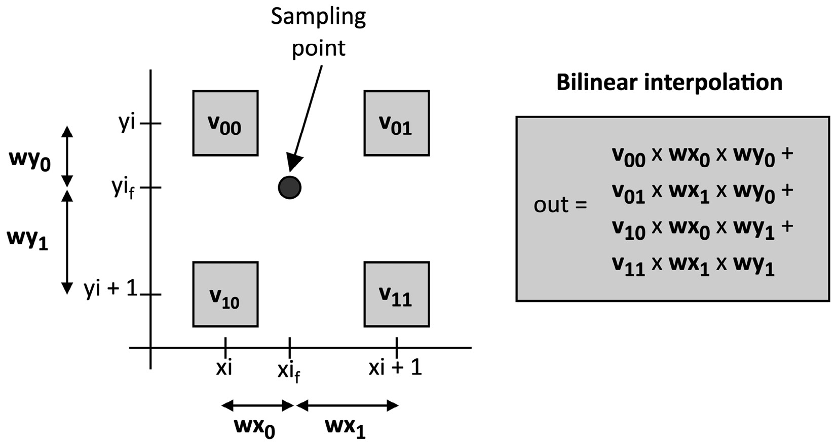
Figure 5.20 – Bilinear interpolation
The interpolation function calculates the output pixel with a weighted average of the four nearest pixels to the input sampling point, as described by the formula in the previous figure.
In our case, we have shown an example of bilinear interpolation applied to a single color component image. However, this method works regardless of the number of color components since we can interpolate the values independently.
How to do it...
Unplug the USB cable from the Arduino Nano and remove the push-button from the breadboard. After that, open the Arduino IDE and copy the sketch developed in the Converting QQVGA images from YCbCr422 to RGB888 recipe in a new project. Next, import the indoor_scene_recognition.h header file into the Arduino IDE.
In the sketch, remove the code in the loop() function and all the references to the push-button usages.
The following are the necessary steps to recognize indoor environments with the Arduino Nano:
- Include the indoor_scene_recognition.h header file:
#include "indoor_scene_recognition.h"
- Include the header files for using the TFLu runtime:
#include <TensorFlowLite.h>
#include <tensorflow/lite/micro/all_ops_resolver.h>
#include <tensorflow/lite/micro/micro_error_reporter.h>
#include <tensorflow/lite/micro/micro_interpreter.h>
#include <tensorflow/lite/schema/schema_generated.h>
#include <tensorflow/lite/version.h>
The header files are the same ones described in Chapter 3, Building a Weather Station with TensorFlow Lite for Microcontrollers.
- Declare the variables related to TFLu initialization/runtime as global:
const tflite::Model* tflu_model = nullptr;
tflite::MicroInterpreter* tflu_interpreter = nullptr;
TfLiteTensor* tflu_i_tensor = nullptr;
TfLiteTensor* tflu_o_tensor = nullptr;
tflite::MicroErrorReporter tflu_error;
constexpr int tensor_arena_size = 144000;
uint8_t *tensor_arena = nullptr;
float tflu_scale = 0.0f;
int32_t tflu_zeropoint = 0;
- The variables reported in the preceding code are the same ones used in Chapter 3, Building a Weather Station with TensorFlow Lite for Microcontrollers, with the only exception being the output quantization parameters since they are not required in this case. The tensor arena size is set to 144000 to accommodate the input, output, and intermediate tensors of the TFLite model.
- Declare and initialize the resolutions of the cropped camera frame and input shape as global variables:
int height_i = 120; int width_i = hi;
int height_o = 48; int width_o = 48;
Since we crop the camera frame before resizing it, we can make cropping simpler by taking a square area matching the height of the camera frame on the left side.
- Declare and initialize the resolution scaling factors to resize the camera frame as global variables:
float scale_x = (float)width_i / (float)width_o;
float scale_y = scale_x;
- Write the function to calculate the bilinear interpolation for a single color component pixel:
uint8_t bilinear_inter(uint8_t v00, uint8_t v01,
uint8_t v10, uint8_t v11,
float xi_f, float yi_f,
int xi, int yi) {
const float wx1 = (xi_f - xi);
const float wx0 = (1.f – wx1);
const float wy1 = (yi_f - yi);
const float wy0 = (1.f - wy1);
return clamp_0_255((v00 * wx0 * wy0) +
(v01 * wx1 * wy0) +
(v10 * wx0 * wy1) +
(v11 * wx1 * wy1));
}
The preceding function calculates the distance-based weights and applies the bilinear interpolation formula described in the Getting ready section of this recipe.
- Write the function to rescale the pixel values from [0,255] to [-1,1]:
float rescaling(float x, float scale, float offset) {
return (x * scale) - offset;
}
Next, write the function to quantize the input image:
int8_t quantize(float x, float scale, float zero_point) {
return (x / scale) + zero_point;
}
Tip
Since rescaling and quantizing are executed one after the other, you may think of fusing them in a single function to make the implementation more efficient in terms of arithmetic instructions executed.
- In the setup() function, dynamically allocate the memory for the tensor arena:
tensor_arena = (uint8_t *)malloc(tensor_arena_size);
We allocate the tensor arena with the malloc() function to place the memory in the heap. As we know, the heap is the area of RAM related to the dynamic memory and can only be released explicitly by the user with the free() function. The heap is opposed to the stack memory, where the data lifetime is limited to the scope. The stack and heap memory sizes are defined in the startup code, executed by the microcontroller when the system resets. Since the stack is typically much smaller than the heap, it is preferable to allocate the TFLu working space in the heap because the tensor arena takes a significant portion of RAM (144 KB).
- Load the indoor_scene_recognition model, initialize the TFLu interpreter, and allocate the tensors: shankar
tflu_model = tflite::GetModel(
indoor_scene_recognition);
tflite::AllOpsResolver tflu_ops_resolver;
tflu_interpreter = new tflite::MicroInterpreter(tflu_model, tflu_ops_resolver, tensor_arena, tensor_arena_size, &tflu_error);
tflu_interpreter->AllocateTensors();
Next, get the pointers to the input and output tensors:
tflu_i_tensor = tflu_interpreter->input(0);
tflu_o_tensor = tflu_interpreter->output(0);
Finally, get the input quantization parameters:
const auto* i_quantization =
reinterpret_cast<TfLiteAffineQuantization*>(
tflu_i_tensor->quantization.params);
tflu_scale = i_quantization->scale->data[0];
tflu_zeropoint = i_quantization->zero_point->data[0];
}
- Iterate over the spatial coordinates of the MobileNet v2 input shape in the loop() function. Then, calculate the corresponding sampling point position for each output coordinate. Next, round down to the nearest integer value the sampling point coordinate:
for (int yo = 0; yo < height_o; yo++) {
float yi_f = (yo * scale_y);
int yi = (int)std::floor(yi_f);
for(int xo = 0; xo < width_o; xo++) {
float xi_f = (xo * scale_x);
int xi = (int)std::floor(xi_f);
As you can observe from the code, we iterate over the spatial coordinates of the MobileNet v2 input shape (48x48). For each xo and yo, we calculate the sampling position (xi_f and yi_f) in the camera frame required for the resize operation. Since we apply bilinear interpolation to resize the image, we round down to the nearest integer xi_f and yi_f to get the spatial coordinates of the top-left pixel in the 2x2 sampling grid.
Once you have the input coordinates, calculate the camera buffer offsets to read the four YCbCr422 pixels needed for the bilinear interpolation:
int x0 = xi;
int y0 = yi;
int x1 = std::min(xi + 1, width_i - 1);
int y1 = std::min(yi + 1, height_i - 1);
int stride_in_y = Camera.width() * bytes_per_pixel;
int ix_y00 = x0 * sizeof(int16_t) + y0 * stride_in_y;
int ix_y01 = x1 * sizeof(int16_t) + y0 * stride_in_y;
int ix_y10 = x0 * sizeof(int16_t) + y1 * stride_in_y;
int ix_y11 = x1 * sizeof(int16_t) + y1 * stride_in_y;
- Read the Y component for each of the four pixels:
int Y00 = data[ix_y00];
int Y01 = data[ix_y01];
int Y10 = data[ix_y10];
int Y11 = data[ix_y11];
Next, read the red-difference components (Cr):
int offset_cr00 = xi % 2 == 0? 1 : -1;
int offset_cr01 = (xi + 1) % 2 == 0? 1 : -1;
int Cr00 = data[ix_y00 + offset_cr00];
int Cr01 = data[ix_y01 + offset_cr01];
int Cr10 = data[ix_y10 + offset_cr00];
int Cr11 = data[ix_y11 + offset_cr01];
After, read the blue-difference components (Cb):
int offset_cb00 = offset_cr00 + 2;
int offset_cb01 = offset_cr01 + 2;
int Cb00 = data[ix_y00 + offset_cb00];
int Cb01 = data[ix_y01 + offset_cb01];
int Cb10 = data[ix_y10 + offset_cb00];
int Cb11 = data[ix_y11 + offset_cb01];
- Convert the YCbCr422 pixels to RGB888:
uint8_t rgb00[3], rgb01[3], rgb10[3], rgb11[3];
ycbcr422_rgb888(Y00, Cb00, Cr00, rgb00);
ycbcr422_rgb888(Y01, Cb01, Cr01, rgb01);
ycbcr422_rgb888(Y10, Cb10, Cr10, rgb10);
ycbcr422_rgb888(Y11, Cb11, Cr11, rgb11);
- Iterate over the channels of the RGB pixels:
uint8_t c_i; float c_f; int8_t c_q;
for(int i = 0; i < 3; i++) {
For each color component, apply bilinear interpolation:
c_i = bilinear(rgb00[i], rgb01[i],
rgb10[i], rgb11[i],
xi_f, yi_f, xi, yi);
Next, rescale and quantize the color component:
c_f = rescale((float)c, 1.f/255.f, -1.f);
c_q = quantize(c_f, tflu_scale, tflu_zeropoint);
In the end, store the quantized color component in the input tensor of the TFLite model and close the for loop that iterates over the spatial coordinates of the MobileNet v2 input shape:
tflu_i_tensor->data.int8[idx++] = c_q;
}
}
}
- Run the model inference and return the classification result over the serial:
TfLiteStatus invoke_status = tflu_interpreter->Invoke();
size_t ix_max = 0;
float pb_max = 0;
for (size_t ix = 0; ix < 3; ix++) {
if(tflu_o_tensor->data.f[ix] > pb_max) {
ix_max = ix;
pb_max = tflu_o_tensor->data.f[ix];
}
}
const char *label[] = {"bathroom", "kitchen", "unknown"};
Serial.println(label[ix_max]);
Compile and upload the sketch on the Arduino Nano. Your application should now recognize your rooms and report the classification result in the serial monitor!