
Fault Tolerance
3.2.1. Fault, Failure, Availability, Reliability
3.4. Typical Module Failure Rates
3.5. Hardware Approaches to Fault Tolerance
3.5.1. The Basic N-Plex Idea: How to Build Failfast Modules
3.5.2. Failfast versus Failvote Voters in an N-Plex
3.6.1. N-Version Programming and Software Fault Tolerance
3.7. Fault Model and Software Fault Masking
3.7.1. An Overview of the Model
3.7.2. Building Highly Available Storage
3.7.2.1. The Structure of Storage Modules
3.7.2.2. Definition of Store and of Store Read and Write
3.7.2.4. Reliable Storage via N-Plexing and Repair
3.7.3. Highly Available Processes
3.7.3.3. Reliable Processes via Checkpoint-Restart
3.7.3.4. Reliable and Available Processes via Process Pairs
3.7.3.5. The Finer Points of Process-Pair Takeover
3.7.3.6. Persistent Processes-The Taming of Process Pairs
3.7.3.7. Reliable Processes plus Transactions Make Available Processes
3.1 Introduction
This chapter presents three views of fault tolerance: the hardware view, the software view, and the global (holistic) view. It sketches the fault-tolerance problem and shows that the presence of design faults is the ultimate limit to system availability; we have techniques that mask other kinds of faults.
After a brief historical perspective, the chapter begins with standard definitions. Next, some empirical studies and measurements of current systems and typical module failure rates are presented. Then hardware approaches to fault tolerance are surveyed. This leads to the issue of software fault tolerance (tolerating software bugs). The bulk of the chapter presents the fault model and software masking techniques typical of non-transactional systems. Transaction processing systems use these more primitive techniques to implement transactional storage, execution, and messages. The chapter then mentions the meta-system design rules (KISS, Murphy’s Law, and end-to-end arguments) and concludes with a discussion of system delusion that demonstrates an end-to-end issue.
The material of this chapter requires some very simple probability theory. For readers who may have forgotten this theory, the chapter begins with a crash course on probability. Readers who already know this material can skip it, but if you do not know it, don’t panic! It is easy.
3.1.1 A Crash Course in Simple Probability
The probability of an event, A, happening in a certain period is denoted P(A). Probabilities range between zero and one. Zero probability means that the event never occurs; one means that the event certainly occurs. The probability that an event, A, does not occur is 1 – P(A). A and B are independent events if the occurrence of one does not affect the probability of the occurrence of the other. Given independent events A and B, consider the following possibilities and their equations:
Both happen. The probability of both A and B happening in that period is the product of their probabilities:
![]()
At least one happens. The probability of at least one of A and B happening is the probability that A happens plus the product of the probability that A does not happen and that B happens:

This equation has a small term P(A) • P(B) that can be ignored if both probabilities are very small.
![]()
For example, if the chance a system fails in a day is .01, the chance the telephone network fails is .02, and the chance the terminal fails is .03, then the chance of all three failing (using Equation 3.1) is .01 • .02 • .03, or 6 • 10−6. The chance of any one of the three failing (using Equation 3.3) is .01 + .02 + .03, or .06.
Failure rates are often memoryless: If the system has been operating for a month, it is no more likely to fail now than it was a month ago. It is as though in each time unit the system flips the failure coin, and with probability P(A) the coin comes up fail; otherwise, the system keeps working without failure. To illustrate: The chance of your dying in the next ten minutes is just about the same as the chance of your dying tomorrow at this time. In the short term, then, your death rate (hazard) is memory less. Of course, when you are 100 years old the hazard function is likely to be higher.
Failure rates are such tiny numbers (say, 10−6) that the reciprocals of the probabilities are used. If the event rate P(A) is memory less and much less than one, the mean time (average time) before the event is expected to occur MT(A) is the reciprocal of the rate, or 1/P(A):
Mean time to event. If the probability P(A) of event A per unit of time is much less than one and is memoryless, then the mean time to event A is the reciprocal of the probability of the event:
![]()
The mean time to failure of the components used in the previous example is 100 days (1/.01) for the system, 50 days (1/.02) for the network, and 33 days (1/.03) for the terminal. The mean time to any of them failing is about 17 days (1/.06), and the mean time to all of them failing is 170,000 days (1/(6 • 10−6)).
System designers are often presented with modules A, B, C, which fail independently and have mean times to failures MT(A), MT(B), MT(C). If they are simply combined into a group G, then the failure of any one is likely to fail the whole group. What is MT(G)? Using Equation 3.3, the probability, P(G), that any one of them fails is approximately P(A) + P(B) + P(C). So, using Equation 3.4:
Mean time to any event. If events A, B, C have mean time MT(A), MT(B), MT(C), then the mean time to the first one of the three events is:
Given N events A, all with the same mean time to occur, MT(A), the mean time to the first event is:
![]()
This is the math needed for this chapter. But, it is very important to understand three key assumptions that underlie these assumptions: (1) The event probabilities must be independent, (2) the probabilities must be small, and (3) the distributions must be memoryless. Exercises 1 and 2 explore these points.
3.1.2 An External View of Fault Tolerance
Fault tolerance is a major concern of transaction processing. Early batch transaction processing systems achieved fault tolerance by using the old master-new master technique, in which the batch of transactions accumulated during the day, week, or month was applied to the old master file, producing a new master file. If the batch run failed, the operation was restarted. To protect against loss or damage of the transaction file (typically a deck of cards), or the master file (typically a tape), an archive copy of each was maintained. Recovery consisted of carefully making a copy of the old master or transaction batch, then using the copy to rerun the batch (see Figure 3.1). Copies of the old masters were retained for five days, then week-old, month-old, and year-old copies were kept. In addition, all transaction inputs were kept. With this data, any old state could be reconstructed.
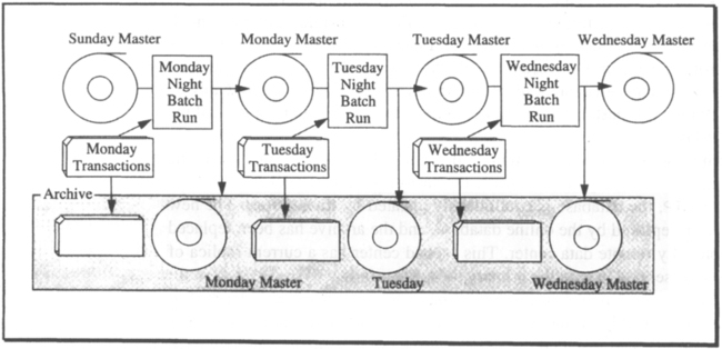
Programs had internal checks to detect missing and incorrect data. When data was corrupted or missing, the redundant data in the old masters and in the transaction histories made it possible to reconstruct a correct current state.
This design tolerated any single failure and could tolerate several multi-failure scenarios. A failure might delay the batch processing, but the system could tolerate any failure short of destruction of both the archive and active copies of the files. In modern terminology, the old master-new master scheme tolerates any single fault; it is single-fault tolerant. It could be made n-fault tolerant by making n + 1 copies of each item, with n + 1 tape drives and operators, and storing them in n + 1 archives. But this was rarely done—single-fault tolerance was usually considered adequate, especially since the master file could probably be reconstructed from the old, old master (the Sunday Master in Figure 3.1) and the log (all the transactions since Sunday).
The more modern version of the same system is shown in Figure 3.2. In that system, the transactions are not batched but are processed while the customer waits. Using online transaction processing, or OLTP, the database is continuously updated by transactions. The new master database has been replaced by the online database, and the archive has been replaced by a second, geographically remote data center. This second center has a current replica of the data and can take over service in case the primary data center fails.

The bank with the system depicted in Figure 3.2 has gone to considerable lengths to provide its customers with a highly available service. It bought dual fault-tolerant data centers, dual telephone networks, and installed dual automated teller machines (ATMs) at each kiosk. In this example, the ATMs are the most unreliable component of the system, yielding about 99% availability. To mask the unreliability of the ATMs, the bank puts two at each customer site. If one ATM fails, the client can step to the adjacent one to perform the task. This is a good example of analyzing the overall system availability and applying redundancy where it is most appropriate.
Figure 3.2 raises the issue of what it means for a system of many components to be available. If the bank in that figure has 10,000 ATM kiosks, some kiosks (pairs of ATMs) will be out of service at any instant. In addition, it is always possible that the database is down, or at least the part that some customer wants to access is unavailable (being recovered). The system is probably never completely “up,” so the concept of system availability becomes:
System availability. The fraction of the offered load that is processed with acceptable response times.
System availability is usually expressed as a percentage. To apply this idea, suppose the ATMs in Figure 3.2 average one unscheduled outage every 100 days, and the problem takes on average a day to fix.1 Such a high failure rate (1%) dominates the system availability. From the customer’s perspective the system availability is 99% (=100% – 1%) without the duplexed ATMs. If the ATMs are duplexed at each site and if they have independent failure modes, then the customer is denied service only if both ATMs are broken. What is the chance of that? Using Equation 3.1, if the probability of one ATM failing in a day is 1%, then the chance of both breaking in the same day is .01% (.01 • .01). The ATM-pair availability is therefore 99.99%. Using Equation 3.4, this is a 10,000-day mean time to both failing. With 10,000 such kiosks, only one would normally be out of service at any instant.
A 99% availability was considered good in 1980, but by 1990 most systems are operating at better than 99.9% availability. After all, 99% availability is 100 minutes per week of denied service. As the nines begin to pile up in the availability measure, it becomes more convenient to think of availability in terms of denial-of-service measured in minutes per year. For example, 99.999% availability is about 5 minutes of service denial per year (see Table 3.3). Even this metric, though, is a little cumbersome so we introduce the concept of availability class, or simply class. This metric is analogous to the hardness of diamonds or the class of a clean room:
Table 3.3
Availability of typical systems classes. In 1990, the best systems were in the high-availability range with Class 5. The best of the general-purpose systems were in the fault-tolerant range.
| System Type | Unavailability(min/year) | Availability | Class |
| Unmanaged | 52,560 | 90.% | 1 |
| Managed | 5,256 | 99.% | 2 |
| Well-managed | 526 | 99.9% | 3 |
| Fault-tolerant | 53 | 99.99% | 4 |
| High-availability | 5 | 99.999% | 5 |
| Very-high-availability | .5 | 99.9999% | 6 |
| Ultra-availability | .05 | 99.99999% | 7 |

Availability class. The number of leading nines in the availability figure for a system or module. More formally, if the system availability is A, the system class is
![]()
Alternatively, the denial-of-service metric can be measured on a system-wide basis or on a per-customer basis. To see the per-customer view, consider the 99% available ATM that denies service to a customer an average of one time in 100 tries. If the customer uses an ATM twice a week, then a single ATM will deny a customer service once a year on average (≈ 2 • 52 weeks = 104 tries). A duplexed ATM will deny the customer service about once every hundred years. For most people, this is the difference between rarely down and never down.
To give a sense of these metrics, nuclear reactor monitoring equipment is specified to be class 5, telephone switches are specified to be class 6, and in-flight computers are specified to be class 9. In practice, these demanding specifications are sometimes met.
3.2 Definitions
Fault tolerance discussions benefit from terminology and concepts developed by an IFIP Working Group (IFIP WG 10.4) and by the IEEE Technical Committee on Fault-Tolerant Computing. The following sections review the key definitions set forth by these organizations.
3.2.1 Fault, Failure, Availability, Reliability
A system can be viewed as a single module, yet most systems are composed of multiple modules. These modules have internal structures consisting of smaller modules. Although this presentation discusses the behavior of a single module, the terminology applies recursively to modules with internal modules.
Each module has an ideal specified behavior and an observed behavior. A failure occurs when the observed behavior deviates from the specified behavior. A failure occurs because of an error, or a defect in the module. The cause of the error is a fault. The time between the occurrence of the error and the resulting failure is the error latency. When the error causes a failure, it becomes effective; before that, the failure is latent (see Figure 3.4).

For example, a programmer’s mistake is a fault. It creates a latent error in the software. When the erroneous instructions are executed with certain data values, they cause a failure and the error becomes effective. As a second example, a cosmic ray (fault) may discharge a memory cell, causing a memory error. When the memory is read, it produces the wrong answer (memory failure), and the error becomes effective.
The observed module behavior alternates between service accomplishment, when the module acts as specified, and service interruption, when the module’s behavior deviates from the specified behavior. These states are illustrated in Figure 3.4.
Module reliability measures the time from an initial instant to the next failure event. Reliability is statistically quantified as mean-time-to-failure (MTTF); service interruption is statistically quantified as mean-time-to-repair (MTTR).
Module availability measure the ratio of service-accomplishment to elapsed time. Availability is statistically quantified as
![]()
3.2.2 Taxonomy of Fault Avoidance and Fault Tolerance
Module reliability can be improved by reducing failures, and failures can be avoided by valid construction and by error correction. The following taxonomy of validation and correction from the IFIP Working Group [Laprie 1985] may help to define the terms.
Validation can remove errors during the construction process, thus ensuring that the constructed module conforms to the specified module. Since physical components fail during operation, validation alone cannot ensure high reliability or high availability. Error correction reduces failures by using redundancy to tolerate faults. Error correction is of two types.
The first type of error correction, latent error processing, tries to detect and repair latent errors before they become effective. Preventive maintenance is an example of latent error processing. The second type, effective error processing, tries to correct the error after it becomes effective. Effective error processing can either mask the error or recover from the error.
Error masking uses redundant information to deliver the correct service and to construct a correct new state. Error correcting codes (ECC) used for electronic, magnetic, and optical storage are examples of masking. Error recovery denies the requested service and sets the module to an error-free state. Error recovery can take two forms.
The first form of error recovery, backward error recovery, returns to a previous correct state. Checkpoint/restart is an example of backward error recovery. The second form, forward error recovery, constructs a new correct state. Redundancy in time, such as resending a damaged message or rereading a disk page, is an example of forward error recovery.
3.2.3 Repair, Failfast, Modularity, Recursive Design
Section 3.7 specifies the correct behavior and some faults of the classic software modules: processes, messages, and storage. A failure that merely constitutes a delay of the correct behavior—for example, responding in one day rather than in one second—is called a timing failure. Faults can be hard or soft. A module with a hard fault will not function correctly—it will continue with a high probability of failing—until it is repaired. A module with a soft fault appears to be repaired after the failure. Soft faults are also known as transient or intermittent faults. Timing faults, for example, are often soft.
Recall that the time between the occurrence of a fault (the error) and its detection (the failure) is called the fault latency. A module is failfast if it stops execution when it detects a fault (stops when it fails), and if it has a small fault latency (the fail and the fast). The term failstop is sometimes used to mean the same thing.
As shown later, failfast behavior is important because latent errors can turn a single fault into a cascade of faults when the recovery system tries to use the latent faulty components. Failfast minimizes fault latency and so minimizes latent faults.
Modules are built recursively. That is, the system is a module composed of modules, which in turn are composed of modules, and so on down to leptons and quarks. The goal is to start with ordinary hardware, organize it into failfast hardware and software modules, and build up a system (a super module) that has no faults and, accordingly, is a highly available system (module). This goal can be approached with the controlled use of redundancy and with techniques that allow the super-module to mask, or hide, the failures of its component modules. Many examples of this idea appear throughout this chapter and this book.
3.3 Empirical Studies
As Figures 3.1 and 3.2 show, there has been substantial progress in fault tolerance over the last few decades. Early computers were expected to fail once a day (very early ones failed even more often). Today it is common for modules, workstations, disks, memories, processors, and so on, to have mean-time-to-failure (MTTF) ratings of ten years or more (100,000 hours or more). Whole systems composed of hundreds or thousands of such modules can offer MTTF of one month if nothing special is done, or 100 years if great care is taken. The following subsections cite some of the empirical data that support this claim.
3.3.1 Outages Are Rare Events
In former times, everyone knew why computers failed: It was the hardware. Now that hardware is very reliable, outages (service unavailability) are rare, and, since much of our experience is anecdotal, patterns are not so easy to discern. The American telephone network had two major problems in 1990. In one outage, a fire in a midwest switch disabled most of the Chicago area for several days; in another outage, a software error clogged the long-haul network for eight hours. The New York Stock Exchange had four outages in the 1980s. It closed for a day because of a snowstorm, it closed for four hours due to a fire in the machine room, it closed 45 seconds early because of a software error, and trading stopped for three hours due to a financial panic. The Internet was accidentally clogged by a student one day, and so on.
If we look at hundreds of events from many different fault-tolerant systems, the main pattern that emerges is that these events are rare—in fact, very rare. Each is the combination of special circumstances. Some patterns do emerge, however, if we look at the sources of failures.
Perhaps the first thing to notice from the anecdotes above, and this is borne out in the broader context as well, is that few of the outages were caused by hardware faults. Fault-tolerance masks most hardware faults. If a fault-tolerant system failed due to a hardware fault, there was probably also a software error (the software should have masked the hardware fault) or an operator error (the operator did not initiate repair) or a maintenance error (all the standby spares were broken and had not been repaired) or an environmental failure (the machine room was on fire). As explained in greater detail in Sections 3.5 and 3.6, hardware designers have developed very simple and effective ways of making arbitrarily reliable hardware, and software designers have developed ways to mask most of the residual hardware faults. As hardware prices plummet, the use of these techniques is becoming standard. Outages (denial of service) can be traced to a few broad categories of causes:
Environment. Facilities failures such as the machine room, cooling, external power, data communication lines, weather, earthquakes, fires, floods, acts of war, and sabotage.
Operations. All the procedures and activities of normal system administration, system configuration, and system operation.
Maintenance. All the procedures and activities performed to maintain and repair the hardware and facilities. This does not include software maintenance, which is lumped in with software.
Hardware. The physical devices, exclusive of environmental support (air conditioning and utilities).
Software. All the programs in the system.
Process. Outages due to something else. Examples are labor disputes (strikes), shutdowns due to administrative decisions (the stock exchange shutdown at panic), and so on.
This taxonomy gives considerable latitude to interpretation. For instance, if a disgruntled operator destroys the system, is the damage due to sabotage (environment) or operations? Sabotage (environment) is probably the correct interpretation, because it was not a simple operations or maintenance mistake. If the system is located in an area of intense electrical storms, but lacks surge protection, is environment or process the cause? Process should probably be held accountable, because the problem has a solution that the customer has not installed.
3.3.2 Studies of Conventional Systems
Given this taxonomy, what emerges from measurements of “real” systems? Unfortunately, that is a secret. Almost no one wants to tell the world how reliable his system is. Since hundreds or thousands of systems must be examined to see any patterns, there is little hope of forming a clear picture of the situation.
The most extensive public study was done by the Japanese Information Processing Development Corporation (JIPDEC) in 1985. It surveyed the outages reported by 1,383 institutions in 1985 [Watanabe 1986]. The institutions reported 7,517 outages, with average durations of 90 minutes, resulting in a MTTF of about ten weeks and an availability of 99.91%. The study is summarized in Figure 3.5.
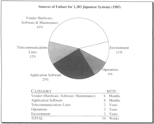
This study is especially interesting since these are not fault-tolerant systems. They are just ordinary computers managed by people who have a justly deserved reputation for careful planning and good quality. These statistics compare favorably with the best numbers reported by comparable groups in the United States, and are better by a factor of ten than typical reports (see, for example, the study by Mourad [1985]).
The categories shown in Figure 3.5 do not correspond exactly to the ones introduced earlier; they lump hardware, vendor software, and vendor maintenance together. But the study shows one thing very clearly: if the vendor provided perfect hardware, software, and maintenance, the system MTTF would be four months (this is an application of Equation 3.5). If the goal is to build systems that do not fail for years or decades, then all aspects of availability must be addressed—simple hardware fault tolerance is not enough.
3.3.3 A Study of a Fault-Tolerant System
A more recent study of a fault-tolerant system provides a similar picture. Unfortunately, the study was based on outages reported to the vendor, and therefore it grossly underreports outages due to environment, operations, and application software. It really captures only the top wedge of the figure above. But since data is so scarce in this area, the results are presented with that caveat. The study covered the reported outages of Tandem computer systems between 1985 and 1990, encompassing approximately 7,000 customer years, 30,000 system years, 80,000 processor years, and over 200,000 disk years. The summary information for three periods is shown in Table 3.6.
Table 3.6
Summary of Tandem reported system outage data.
| 1985 | 1987 | 1989 | |
| Customers | 1,000 | 1,300 | 2,000 |
| Outage Customers | 176 | 205 | 164 |
| Systems | 2,400 | 6,000 | 9,000 |
| Processors | 7,000 | 15,000 | 25,500 |
| Disks | 16,000 | 46,000 | 74,000 |
| Reported Outages | 285 | 294 | 438 |
| System MTTF | 8 years | 20 years | 21 years |

Table 3.6 summarizes the statistical base, and Figures 3.7 and 3.8 display the information by category. They show the causes of outages and the historical trends: Reported system outages per 1,000 years (per millennium) improved by a factor of two by 1987 and then held steady. Most of the improvement came from improvements in hardware and maintenance, which together shrank from 50% of the outages to under 10%. By contrast, operations grew from 9% to 15% of outages. Software’s share of the problem got much bigger during the period, growing from 33% to more than 60% of the outages.

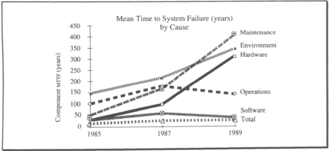
Figure 3.7 seems to imply that operations and software got worse, but that is not the case. Figure 3.8 shows that software and operations MTTF stayed about constant, while the other fault sources improved considerably.
Two forces explain the maintenance improvements: technology and design. Disks give the best example of both forces. In 1985, each disk had to be serviced once a year. This involved powering down the disk, replacing an air filter, adjusting the power system, and sometimes adjusting head alignment. In addition, the typical 1985 disk required one unscheduled service call per year for repair. This resulted in 32,000 tasks per year in 1985 for customer engineers, and it created many opportunities for mistakes. In addition, the disk cabinets and connectors were not designed for maintenance, rendering maintenance tasks awkward and requiring special tools. If technology and design had not changed, engineers would have been performing 150,000 maintenance tasks per year in 1989—the equivalent of 175 full-time people just doing the error-prone task of disk maintenance.
Instead, 1990-vintage disks have no scheduled maintenance. Fiber-optic connectors reduce cabling and connectors by a factor of 20, and installation and repair require no tools (only thumb screws are used). All field-replaceable units have built-in self-test and light-emitting diodes that indicate correct operation. In addition, disk MTTF rose from 8,000 hours to over 100,000 hours (observed) since 1985. Disk controllers and power supplies experienced similar dramatic improvements. The result was that the disk population grew ba factor of five while the absolute number of outages induced by disk maintenance shrank by a factor of four—a 2,000% improvement. Almost all the reported disk maintenance problems were with older disks or were incident to installing new disks.
This is just one example of how technology and design have improved the maintenance picture. Since 1985, the size of Tandem’s customer engineering staff has held almost constant and shifted its focus from maintenance to installation, even while the installed base tripled. This is an industry trend; other vendors report similar experience. Hardware maintenance is being simplified or eliminated.
Other hardware experienced a similar improvement in MTTF. Based on Table 3.6, during 1989 there were well over 30,000 hardware faults, yet only 29 resulted in a reported system outage. The vast majority were masked by the software (the Tandem system is single-fault tolerant, requiring two hardware faults to cause an outage). The MTTF of a duplexed pair goes up as the square of the MTTF of the individual modules (see Section 3.6). Thus, minor changes in module MTTF can have a dramatic effect on system MTTF. The clear conclusion is that hardware designers did a wonderful job. Hardware faults were rare, and all but 4% of the ones that did occur were masked by software.
While hardware and maintenance show a clear trend toward improvement, operations and software did not improve. The reason for this lies in the fact that few tools were provided to the operators; thus there is no reason to expect their performance to have changed. According to Figure 3.8, every 150 system-years some operator made a mistake serious enough to crash a system. Clearly, mistakes were made more frequently than that, but most operations mistakes were masked by the system, which has some operator fault tolerance.
Operations mistakes were split evenly between two broad categories: configuration and procedures. Configuration mistakes involve such things as having a startup file that asks the transaction manager to reinitialize itself. This works fine the first time the system starts, but it causes loss of transactions and data integrity when the system is restarted from a crash. Mixing incompatible software versions or using an old version of software are common configuration faults. The most common procedural mistake is letting the system fill up by allowing a file to get so big that either there is no more disk space for it or no new records can be added to it.
No clearer pattern of operations faults emerges from the Tandem study. The basic problem of improving operations is that the only known technique is to eliminate or automate the operations process, replacing operators with software.
As Figure 3.7 shows, software is a major source of outages. The software base (number of lines of code) grew by a factor of three during the study period, but the software MTTF held almost constant. This reflects a substantial improvement in software quality. But if these trends continue, the software will continue to grow at the same rate that the quality improves, and software MTTF will not improve. The software in this study uses many of the software fault tolerance techniques described later in this chapter. But that is not enough; a tenfold improvement in software quality is needed to achieve Class 5 availability. At present, no technique offers such an improvement without huge expense. Section 3.6 surveys the most effective approaches: N-version programming and process-pairs combined with transactions.
Thus far, we examined the failure rates of whole systems. We now look at typical failure rates for system components such as processors, disks, networks, and software.
3.4 Typical Module Failure Rates
System designers need rules of thumb for module failure modes, rates, and repair times. There are huge variations among these. Intervals between failures seem to obey exponential, or even hyper-exponential distributions. This makes talking about averages deceptive. In addition, failure rates often vary over time, following a bathtub curve (see Figure 3.9). The rate in the beginning, often called the burn-in rate, is high. After that, the rate remains low and nearly constant for many years. Then the device begins to age mechanically, or wear out, and the rate rises. Failure rates are usually quoted for the bottom of the bathtub curve. To mask burn-in, manufacturers often operate modules for a few hours or days to detect burn-in faults. Only modules passing this burn-in period are sent to customers.

Two kinds of failure rates are of interest: quoted and observed. Quoted failure rates are those promised by the vendor, while observed failure rates are those seen by the customer. For phone lines and for some modules, the observed numbers are much better than the quoted numbers because the quoted numbers are often guarantees, and the customer has a right to complain if the rate falls below the quoted rate. MTTF is usually quoted in hours, generally with only the first digit significant. Often only the magnitude of the MTTF is significant, so that 10,000 hours could actually be 7,000 or 12,000. With about 8,760 hours in a year, each year has about 10,000 hours. A 50,000-hour MTTF, therefore, means about a 5-year MTTF. Given these very approximate measures, here are some typical MTTFs:
Connectors and cables. Connectors and cables are commonly rated at 1,000 years MTTF. Their failure modes are corrosion of contacts, bent connector pins, and electrical erosion. Connectors and cables have high burn-in failure rates.
Logic boards. Depending on cooling, environment, and internal fault masking, logic boards are rated at between 3 and 20 years MTTF. The ratio of soft to hard faults varies from a low of 1:1 to 5:1 (typical) to greater than 10:1 for badly designed circuits.
Disks. Workstation and PC disks are notoriously unreliable (one-year MTTF observed), whereas “expensive disks” are quite reliable (rated at 5 years, with over 20 years MTTF observed). Table 3.10 gives these statistics (the term ECC refers to the extensive error correcting codes found in disk controllers to mask bad spots on the disk). Recent (June 1990) reports of IBM drives report 570 months MTTF for a population of 3,889 drives. This is approximately a 50-year MTTF. These drives will be obsolete long before they wear out or fail.
Table 3.10
mttf of various disk failures [Schulze 1989].
| Type of Error | MTTF | Recovery | Consequences |
| Soft data read error | 1 hour | Retry or ECC | None |
| Recoverable seek error | 6 hours | Retry | None |
| Maskable hard data read error | 3 days | ECC | Remap to new sector and rewrite good data |
| Unrecoverable data read error | 1 year | None | Remap to new sector, old data lost |
| Device needs repair | 5 years | Repair | Data unavailable |
| Miscorrected data read error | 107 years | None | Read wrong data |

Workstations. Workstation reliability varies enormously. The marketplace is extremely competitive, and manufacturers often economize by having inadequate power, cooling, or connectors. A minimal good-quality terminal is usually rated at three to five years (the display is often the weak link). Workstation hardware is usually rated at one to five years, disks often being the weak link. Workstation software seems to have a two-week MTTF [Long 1990].
Software. Production software has ≈3 design faults per 1,000 lines of code. Most of these bugs are soft; they can be masked by retry or restart. The ratio of soft to hard faults varies, but 100:1 is usual (see Subsection 3.6.2).
Data communications lines (USA). The telephone systems of North America and northern Europe are among the most reliable systems in the world. They are spectacularly well managed and provide admirable service. (The story is not so pleasant elsewhere.) With the advent of fiber optics, line quality is getting even better. Line quality is measured in error-free seconds. Raw fiber media rates are 10−9 BER (bit error rate). This suggests that one message in a million is lost. When all the intermediate components are added, error rates often rise to 10−5. If a message is about a kilobit, this suggests that 1:100 or 1:1000 messages are corrupted. These are soft error rates. Hard errors (outages) vary enormously and are clustered in bursts. Suppliers usually promise 95% error-free seconds, 10−6 BER, and 99.7% availability. There are frequent dropouts of 100 ms or less when no good data is transmitted. Duplexing the lines via independent paths should mask almost all such transient faults. Such duplexing is a service provided in most countries.
LANs. Raw cable and fiber are rated at 10−9 BER and 10−6 bad messages per hour. Most LAN problems arise from protocol violations or from overloads. One study of an Ethernet LAN over a 7-month period observed nine overload events due to broadcast storms, thrashing clients, babbling nodes, protocol mismatch, and analog noise [Maxion 1990]. This suggests a 3-week MTTF.
Power failures. Power is the most serious problem outside Japan and northern Europe. Based on Table 3.11, any system wanting MTTF measured in years should carefully condition its input power and should install a local uninterruptible power supply. In one study of a North American customer who did not do this, 75% of unscheduled outages were related to power failure. Table 3.11 summarizes the rates.
Table 3.11
Frequency and average duration of power outages in Europe and North America. Power in Japan is reputed to be comparable to that in Germany. Power in the Third World is reputed to be worse than that in Italy. Areas with severe electrical storms should expect much worse service. These numbers do not include sags (outages of less than a second) and surges (over-voltages that can burn out equipment). North American source is Tullis [1984].
| Out min/year | Events/year | Avg event(min) | ||
| North America | 125 | 2.3 | 54 | |
| England | 67 | 0.72 | 92 | |
| France | urban | 33 | 0.8 | 41 |
| rural | 390 | 5 | 78 | |
| Germany | urban | 7 | 0.33 | 20 |
| rural | 54 | 1.2 | 45 | |
| Italy | urban | 120 | 2.5 | 48 |
| rural | 300 | 5 | 60 |

These statistics indicate how frequently modules fail. The other important number is how quickly they are repaired. How long does it usually take a system to be repaired? Several studies indicate that two hours is a typical module repair time if the site is near a service center and reservoir of spare parts. Once repair is complete, the system must initiate recovery. The network probably will have shut down by then (most time-outs are less than two hours). One end-to-end indication of system repair times is the Japanese study mentioned previously (see Figure 3.5), which reported an average of 90 minutes. Another study of outage durations reports a median and mean of twice that (see Figure 3.12)—essentially two hours to diagnose and repair the system and about one hour to bring the application and network back to full operation.

Based on Figure 3.12, outages roughly follow a Poisson distribution. The distribution, however, has a very long tail, since long outages are over-represented.
The statistics in this section tell us that modules fail. The question, then, is how can we build a highly reliable system out of imperfect modules? The next few sections present the various approaches to this problem. First, the hardware approach is covered, then fault-tolerant and failfast software, and finally software masking of software and hardware faults.
3.5 Hardware Approaches to Fault Tolerance
John von Neumann pioneered the idea of building fault-tolerant computer systems. Starting with unreliable components, a model of neurons, he did a design for the human mind (a giant brain) with a 60-year MTTF. His charming and seminal paper concludes that the design requires a redundancy of about 20,000: 20,000 wires in each bundle and 20,000 neurons making each decision. Such redundancy was needed in his view, because he considered any fault in the system as a failure. His system had only one level of modularity, it lacked the notion of failfast, and it lacked the notion of repair. These three ideas and their interaction are extremely important. Because they allow computer systems to get by quite well with 104 times lower redundancy (2 rather than 20,000), they are well worth understanding.
3.5.1 The Basic N-Plex Idea: How to Build Failfast Modules
Failfast modules are easily constructed from ordinary hardware. The simplest design, called pairing or duplexing, connects the inputs and outputs of two modules to a comparator that stops if the module outputs disagree; this is the failfast aspect of the design. Although a pair fails about twice as often as a single module, a failfast module gives clean failure semantics; it also reduces the number of cases fault-tolerant software needs to deal with by converting all failures to a very simple class: stopping. To provide both failfast behavior and increased module MTTF, modules are n-plexed, and a voter takes a majority of their outputs. If there is no majority, the voter stops the n-plex module. The most common case in the n-plex design in which n is greater than 2 (n = 2 is simply pairing) is n = 3. This is generally called triple module redundancy, or TMR. The double and triple redundancy cases are shown in Part A of Figure 3.13.

The basic n-plex design generalizes to a recursive one that allows failfast modules to be aggregated into bigger failfast modules, and that tolerates voter failures and connector failures. In that design, each n-plexed module has n voters and n outputs (see Part B of Figure 3.13).
3.5.2 Failfast versus Failvote Voters in an N-Plex
As the voting scheme is described in the previous section, the voter requires that a majority of the modules be available. If there is no majority, the voter stops. This is called failvote. An alternative scheme, called either failfast voting or failfast represents a fundamental refinement. This scheme has the voter first sense which modules are available and then use the majority of the available modules. Thus, a failfast voter can operate with less than a majority of the modules.
If each of the component modules is failfast, then a failfast voter can operate by observing the outputs of the non-faulty modules. In theory, a voter combining the outputs of failfast sub-modules never detects a mismatch; it just detects missing votes from failed modules. For example, disk modules are usually assumed to be failfast. A failfast voter managing a pair of disks can detect disk failures and can still operate if only one of the two disks is functional. This permits the supermodule (disk pair) to function with only one module.
Even if the component modules are not failfast, the voter can still operate with failfast voting. To do so, a module is marked as failed each time it miscompares, and the voter ignores its inputs until it is repaired. Thus the voter forms a majority from the non-faulty modules. Take as an example a 10-plexed module composed of ordinary (not necessarily failfast) modules. A failvote voter operating the 10-plex will fail when five modules have failed. A failfast voter will continue operating until the ninth module fail, because a failfast voter on non-failfast modules requires only two available modules to operate. This indicates that fail-fast voting has better reliability than failvote voting.
Consider a failvote n-plex and ignore failures of the voters (comparators) and connectors. (For the scenario that follows, refer to Figure 3.14.) Given modules, each of which is failfast, with an MTTF of 10 years, the MTTF of the paired supermodule is about five years (10/2 years, using Equation 3.6).2 The MTTF for the triplex system is about 8.3 years (using Equation 3.6, it is 10/3, or about 3.3 years to the first failure and 10/2, or 5 years to the second and fatal failure). The analysis of pair-and-spare is a little more tricky, since the first pair will fail the first time one of the four processors fails. Equation 3.6 says that is expected to happen in 10/4, or 2.5 years. After one pair fails, the remaining pair is expected to operate for five years, as computed here. Thus, pair and spare has a 7.5-year MTTF. This logic (simply adding the times), incidentally, shows how the memoryless property simplifies analysis.

So far, all this redundancy does not look like a good idea. All three schemes cut the MTTF, making failure more likely. However, there are two extenuating circumstances. First, and most important, n-plexing yields failfast modules. Failfast modules have vastly simplified failure characteristics; they either work correctly or they stop. This simplicity makes it possible to reason about their behavior. If modules can have arbitrary failure behavior, there is little hope of building fault-tolerant systems.
The second benefit of triplexing and pair-and-spare is that if soft (transient) faults dominate, then pair-and-spare or TMR can be a big improvement (recall that modules continue to function after soft errors). Both schemes mask virtually all soft faults, and two of the three would have to have exactly the same fault for the voter to pass on the faulty result. Thus if the ratio of hard faults to total faults is 1:100, and if TMR masks all transient faults, the module MTTF rises by a factor of 100 to become 1,000 years MTTF; in addition, TMR failvote improves the MTTF from about 8.3 years to about 8,333 (≈10,000 • (1/3 + 1/2)) using Figure 3.14).
3.5.3 N-Plex plus Repair Results in High Availability
The key to getting this hundred-fold MTTF improvement is repairing the faulted module immediately after the fault. If the module has no internal state, recovery from a soft fault is easy; the module goes on to compute the next state from its next inputs. But typically, the faulted module is a processor or memory with an incorrect internal state. To repair it, the design must somehow resynchronize the faulted module with the other two modules. The easy way to do this is to reset all the modules to their initial states, but this will probably reflect the fault outside the module. Mechanisms to resynchronize the faulted module without disrupting the service of the other two modules are usually complex and ad hoc. For storage modules, such mechanisms consist of rewriting the state of the faulted storage cell. For processing modules, they generally set the state (registers) of the faulted processor to the state of one of the good processors.
The huge benefit of tolerating soft faults is just one aspect of the key to availability: repair. Soft errors postulate instant mean time to module repair; when the module faults, it is instantly repaired. Failvote duplex and failfast TMR both provide excellent reliability and availability if repair is added to the model.
The failure analysis of a failvote n-plex is easy to follow. Each module goes through the cycle of operation, fault, repair, and then operation again. The supermodule (the n-plex module) will fail if all the component modules fail at once. More formally, the n-plex will fail if all but one module are unavailable, and then the available module fails. The analysis first determines the probability that a particular module, N, will be the last to fail (all others have already failed and are still down). The probability that a particular module is unavailable is
![]()
Using Equation 3.1 with Equation 3.7, the probability that the other n – 1 modules are unavailable is then
![]()
Using Equation 3.4, the probability that a module, N, fails is
![]()
Equation 3.1 can combine Equations 3.8, and 3.9 to compute the probability that the last module N fails, and that all the other modules are unavailable:
![]()
This is the probability that module N causes the n-plex failure. There are n such identical modules. To compute the probability that any one of these n modules causes an n-plex failure, Equation 3.10 is combined n times using Equation 3.3:
![]()
Equation 3.11 is therefore the probability that a failvote n-plex will completely fail. Using Equation 3.4 with Equation 3.11 gives the mean time to total failure for a failfast n-plex:
![]()
Applying Equation 3.12 and using the 1-year MTTF with a 4-hour MTTR,
![]()
The corresponding result for a TMR group is
![]()
Starting with two modest one-year MTTF modules, we have now built a one-millennium module! Thousands of these could be used to build a supermodule with a one-year MTTF. The construction can be repeated to obtain a system with a one-millennium MTTF—a powerful idea (see Table 3.15).
Table 3.15
mttf estimates for various architectures using 1-year mttf modules with 4-hour mttr. Note: in the cost column, the letter ε represents a small additional cost.
| MTTF | Equation | Cost | |
| Simplex | 1 year | MTTF | 1 |
| Duplex: failvote | ≈0.5 years | ≈MTTF/2 | 2+ε |
| Duplex: failfast | ≈1.5 years | ≈MTTF(3/2) | 2+ε |
| Triplex: failvote | ≈.8 year | ≈MTTF(5/6) | 3+ε |
| Triplex: failfast | ≈1.8 year | ≈MTTF(11/6) | 3+ε |
| Pair and Spare: failvote | ≈7 year | ≈MTTF(3/4) | 4+ε |
| Triplex: failfast with repair | >10years | ≈MTTF/3MTTR | 3+ε |
| Duplex failfast + repair | >10 years | ≈MTTF/2MTTR | 2+ε |

3.5.4 The Voter’s Problem
There is a nasty flaw in the previous reasoning: Namely, the assumption that the voters and connectors are faultless. The recursive construction was careful to replicate the voters and connectors for this very reason, so that the construction actually tolerates failures in connectors and voters. Fundamentally, however, system reliability and availability are limited by the reliability of the top-level voters.
In some situations, voting can be carried all the way to the physical system. For example, by putting three motors on the airplane flaps or reactor rods and having them “vote” at the physical level, two can overcome the force of the third. Often the voter cannot be moved to the transducer. In those situations, the message itself must be failfast—it must have a checksum or some other consistency check—and the client must become the voter. Two examples of moving the voter to the client appear in Figure 3.16.

The first example in Figure 3.16 is a repetition of the banking system depicted in Figure 3.2. It shows the failure rates for the various system components and indicates that the ATM is the least reliable component. But using the pair-and-spare scheme produces instant repair times (repair in the sense of providing service): If one ATM fails, the client can step to the adjacent ATM. That moves the voter into the customer. If each ATM is failfast, the customer can operate with a correct one.
The second example in Figure 3.16 shows a disk pair. Data is read from either disk and written to both. Each disk and each controller is a failfast module. In addition, the wires are failfast, because the messages they carry are checksum protected. If the message checksum is wrong, the message is discarded. But the client (the processor in this case) must try the second channel (the second path) to the device if the first fails, much as the bank client must try the second ATM if the first fails. These are both examples of moving the voter into the client.
3.5.5 Summary
The foregoing presentation is from the traditional perspective of hardware fault tolerance. The next two sections develop similar ideas from a software perspective. To bridge these two perspectives, it is important to see the following connections:
Failfast is atomic. Failfast means that a hardware (or software) module either works correctly or does nothing. This is the atomic, all-or-nothing aspect of the ACID property (the A in ACID). Atomicity vastly simplifies reasoning about the way a system will fail.
Failfast is possible. There may be skepticism that it is possible to build failfast modules, but Figure 3.13 shows how to build arbitrarily complex hardware systems with the failfast property through suitable use of redundancy.
Reliable plus repair is consistent and durable. If modules fail and are repaired, then a module will always make correct state transitions (eventually), and the module state will be durable. The module will eventually be repaired and continue service. Consistent and durable are represented by the C and D of ACID.
To summarize, reliability plus repair means doing the right thing eventually; the module may stop, but eventually it is repaired and continues to function. Failfast is the A of ACID, and reliability plus repair are the A, C, and D of ACID. High availability modules can be built by n-plexing failfast modules and by using a failfast voting scheme.
Historically, transaction processing systems have been geared toward reliability—never losing the database. But for many reasons, they often delivered poor availability. Many TP systems were designed in an era when one failure per day was considered typical and when 98% availability was considered high. Technology advances and declining hardware prices have shifted the emphasis from reliability to availability, which means doing the right thing and doing it on time. Repair is the key to reliability, since with enough repair the job eventually gets done. Instant repair is the key to high availability: It almost always masks the failure such that module failures do not cause a denial of service. Combined with failfast, instant repair makes all single faults appear to be soft faults. Both TMR and pair-and-spare provide instant MTTR for hardware faults. These techniques make it possible to buy conventional components off the shelf and combine them to build super-reliable and super-available modules. The next sections show how to achieve instant software MTTR, implying highly available software systems.
3.6 Software Is the Problem
Both the Japanese study and the Tandem study of the causes of system failures point to software as a major source of problems (Subsection 3.3.2). There is a clear trend toward using software to mask hardware, environmental, operations, and maintenance faults. Thus, as all the other faults are masked, the software residue remains. In addition, software is being used to automate operations and simplify maintenance. All this implies millions of new lines of code. In general, production programs engineered using the best techniques (structured programming, walk-throughs, careful code inspections, extensive quality assurance, alpha and beta testing) have two or three bugs per thousand lines of code. Using this rule of thumb, a few million lines of code will have a few thousand bugs—megalines have kilobugs.
It is important to realize that perfect software is possible—it’s just a matter of time and money. The following program, for example, is perfect at adding unsigned integers modulo the machine word size:

As an amusing side note, our first version of this program had two bugs! It advertised add rather than modulo word size add, and it used signed integers, which meant it would get overflow and underflow traps on some machines. Now that it has been through QA, it is a perfect program: It does what it says it does.
Writing perfect software takes time for careful design, and money to pay for it. The U.S. space shuttle software is a case in point. At present, it costs $5,000 per line of code. This price3 includes careful design, code reviews, testing, and then more testing. Yet each time a shuttle flies, the pilots are given a known bug list. One such bug was that if two people typed on two keyboards at the same time, the input buffer would get the OR of the two keyboard inputs (the workaround was to only use one keyboard at a time). How could such a gross error get past such an expensive test process? Obviously, the U.S. government did not have enough time and money. No one, though, has more time and money than the U.S. government, which means that for practical purposes, perfect software of substantial complexity is impossible until someone breeds a species of super-programmers.
Few people believe design bugs can be eliminated. Good specifications, good design methodology, good tools, good management, and good designers are all essential to quality software. These are the fault-prevention approaches, and they do have a big payoff. However, after implementing all these improvements, there will still be a residue of problems.
3.6.1 N-Version Programming and Software Fault Tolerance
The main hope of dealing with design faults is for designers to develop techniques to tolerate design faults, much as hardware designers are able to tolerate hardware faults. Of course, hardware design is software, so hardware designers have the same problem: Their techniques to tolerate physical hardware faults do not mask design faults. There are two major software fault tolerance techniques:
N-version programming. Write the program n times, test each program carefully, and then operate all n programs in parallel, taking a majority vote for each answer. The resulting design diversity should mask many failures.
Transactions. Write each program as an ACID state transformation with consistency checks. At the end of the transaction, if the consistency checks are not met, abort the transaction and restart. Rerunning the transaction the second time should work.4
Both these approaches are statistical and both have merit, but both can fail if there is a fault in the original specification.
The n-version programming approach is expensive to implement and to maintain. That is because to get a majority, n must be at least 3. In addition, the n-version programming approach suffers from the “average IQ” problem. If n students are given a quiz, all of them will get the easy problems right, some will get the hard problems right, and almost none will get the hardest problem right (if it is a good quiz). Also, several will make the same mistakes. An n-version program taking this quiz would score in the 60th percentile. It would solve all the easy problems and might even solve a few of the harder problems. However, there would be no consensus, or consensus would be wrong, on the hardest problems.
A final problem with n-version programming is that module repair is not trivial. Since each module has a completely different internal state, one cannot simply copy the state of a good module to the state of a failing module. Without repair, n-plexing has a worse MTTF than simplexing (see Table 3.15).
N-version programming is often used in high-budget projects employing many low-budget programmers. You can imagine the controversy surrounding this idea. Better results might be obtained by spending three times more on better-quality programmers and on better infrastructure, or on more careful testing of one program.
3.6.2 Transactions and Software Fault Tolerance
Transactions are even more of a gamble. When a production computer system crashes due to software, computer users do not wait for the software to be fixed. They don’t wait for the next release, but instead restart the system and expect it to work the next time; after all, they reason, it worked yesterday. By using transactions, a recent consistent system state is restored so that service can continue. The theory is that it was a Heisenbug that crashed the system. A Heisenbug is a transient software error (a soft software error) that only appears occasionally and is related to timing or overload. Heisenbugs are contrasted to Bohrbugs which, like the Bohr atom, are good, solid things with deterministic behavior.
Although this is preposterous, the test of a theory is whether it explains the facts—and the Heisenbug theory does explain many observations. For example, a careful study by Adams [1984] of all software faults of large IBM systems over a five-year period showed that most bugs were Heisenbugs. The Adams study dichotomized bugs into benign bugs—ones that had bitten only one customer once—and virulent bugs—ones that had bitten many customers or had bitten one customer many times. The study showed that the vast majority (well over 99%) of the bugs were benign (Heisenbugs). Adams also concluded from this study that customers should not rush to install bug fixes for benign bugs, as the expense and risk are unjustified.
There are several other instances of the Heisenbug idea. Most large software systems have data structure repair programs that traverse data structures, looking for inconsistencies. Called auditors by AT&T and salvagers by others, these programs heuristically repair any inconsistencies they find. The code repairs the state by forming a hypothesis about what data is good and what data is damaged beyond repair. In effect, these programs try to mask latent faults left behind by some Heisenbug. Yet, their techniques are reported to improve system mean times to failure by an order of magnitude (for example, see the discussion of functional recovery routines in Mourad [1985] or in Chapter 8 of this book).
Heisenbug proponents suggest crashing the system and restarting at the first sign of trouble; this is the failfast approach. It appears to make things worse, since the system will be crashing all the time, and the database and network will be corrupted when the system is restarted. This is where transactions come in. Transactions, and their ACID properties, have four nice features:
Isolation. Each program is isolated from the concurrent activity of others and, consequently, from the failure of others.
Granularity. The effects of individual transactions can be discarded by rolling back a transaction, providing a fine granularity of failure.
Consistency. Rollback restores all state invariants, cleaning up any inconsistent data structures.
These features mean that transactions allow the system to crash and restart gracefully; the only thing lost is the time required to crash and restart. Transactions also limit the scope of failure by perhaps only undoing one transaction rather than restarting the whole system. But the core issue for distributed computing is that the whole system cannot be restarted; only pieces of it can be restarted, since a single part generally doesn’t control all the other parts of the network. A restart in a distributed system, then, needs an incremental technique (like transaction undo) to clean up any distributed state. Even if a transaction contains a Bohrbug, the correct distributed system state will be reconstructed by the transaction undo, and only that transaction will fail.
The programming style of failfast software designs is called defensive programming by analogy with the defensive automobile driving style advocated by traffic-safety experts. Defensive programming advocates that every software module check all its inputs and raise an exception if the inputs are incorrect. This essentially makes the software module failfast. The module checks all its parameters, and as it traverses internal data structures it checks their integrity. To give a specific example, a program traversing a doubly linked list checks the back-pointer in the next block to be sure that it points to the previous block, and the program checks other redundant fields in the block for sanity. If a list element does not satisfy these tests, then an error has been detected, and it is repaired by discarding the block or by repairing it. Whenever a module calls a subroutine, the callee checks the parameters for sanity, and the caller checks the routine’s results. In case an error is found, an exception handler is invoked. Exception handlers are much like the repair programs mentioned earlier in this section. The exception handler either masks the exception (if it is an internal inconsistency that can be repaired), or the module reflects the exception back to the caller (if it is the caller’s error). In extreme cases, the exception handler cannot mask the fault and, consequently, reflects it as a transaction abort, a subsystem restart, or another coarse form of recovery.
Failfast creates a need for instant crash and restart. This again may seem a preposterous approach, but computer system architectures are increasingly adopting this approach. The concept of process pair (covered in Subsection 3.7.3) specifies that one process should instantly (in milliseconds) take over for the other in case the primary process fails. In the current discussion, we take the more Olympian view of system pairs, that is two identical systems in two different places. The second system has all the data of the first and is receiving all the updates from the first. Figure 3.2 has an example of such a system pair. If one system fails, the other can take over almost instantly (within a second). If the primary crashes, a client who sent a request to the primary will get a response from the backup a second later. Customers who own such system pairs crash a node once a month just as a test to make sure that everything is working—and it usually is.
If Heisenbugs are the dominant form of software faults, then failfast plus transactions plus system pairs result in software fault tolerance. Geographically remote system pairs tolerate not just Heisenbugs, but many other problems as well. They tolerate environmental faults, operator faults, maintenance faults, and hardware faults. Two systems in two different places are not likely to have the same environmental problems: They are on different power grids, different phone grids, and different earthquake faults, and they have different weather systems overhead. They have independent operations staffs, different maintenance personnel, and different hardware. All this means that the two systems have largely independent failure modes. Section 12.6 develops the concept of system pairs in more detail.
3.6.3 Summary
Software faults are the dominant source of system failures. All other faults can be masked with a combination of redundancy, geographic diversity, and software to automate tasks. Software can automate system operations and mask operations and maintenance failures. Software faults, however, remain an unsolved problem.
There are two approaches to software fault tolerance: n-version programming and transactions. The two approaches could be combined. Advocates of n-version programming aim to combine several incorrect programs into a better, more reliable one. N-version programming may also be a good way to write failfast programs. Transaction advocates aim to detect incorrect programs and minimize their effects by undoing them. Transactions encourage a failfast design by allowing the system to quickly crash and restart in the most recent consistent state. By having a standby system, restart can begin within milliseconds.
3.7 Fault Model and Software Fault Masking
The application of the pair-and-spare or n-plex techniques to software modules is not obvious. How do you pair-and-spare a software module? How do you n-plex messages, remote procedure calls, and the like? The answer to these questions—process pairs—is neither trivial nor a direct application of the hardware n-plex and pair-and-spare approaches described in the previous section. To the authors’ knowledge, the best approach to process pairs was worked out in an unpublished classic written by Butler Lampson and Howard Sturgis in 1976 at Xerox. At about the same time Joel Bartlett designed and implemented similar ideas for Tandem’s Guardian operating system. The Lampson-Sturgis model has widely influenced subsequent work in the field; but, unfortunately it is not widely available. Bartlett’s work is even more inaccessible. The presentation here borrows heavily from those original works. The process pair discussion comes from experience with Bartlett’s design.
Designing fault-tolerant programs requires a model. The model must define correct behavior, and if the programs are to deal with faults, the model must describe the kinds of faults and their relative frequencies. Given such a model, programs can be written, system reliability can be estimated using probabilistic methods, and proofs that the programs are correct can be made with any desired degree of formality. The validity of the model cannot be established by proof, since there is no formal model of reality. The strongest possible claim is that the physical system behaves like the model with probability p, and that p is very close to 1. This claim can only be established empirically, by estimating p from measurements of real systems.
The model here involves three entity types: processes, messages, and storage.5 Each has a set of desired behaviors and a set of failure behaviors. This section shows how to transform each of the three entities from failfast entities into highly reliable and even highly available entities.
Faulty behavior is dichotomized into expected faults (those tolerated by the design), and unexpected faults (those that are not tolerated). Unexpected faults can be characterized as dense faults or Byzantine faults:
Dense faults. The algorithms will be n-fault tolerant. If there are more than n faults within a repair period, the service may be interrupted.
Byzantine faults. The fault model postulates certain behavior—for example it may postulate that programs are failfast. Faults in which the system does not conform to the model behavior are called Byzantine.
It is highly desirable that the system be failfast in the dense fault cases. That is, if there are more than n-faults in the repair window, the system should stop rather than continue the computation in some unspecified way. It is possible to measure the rate of unexpected faults in real systems and observe that the rate is small. Some representative measurements appeared in Sections 3.3 and 3.4.
Picking the model is a very painful and delicate process. One is constantly tom between simplicity and completeness. For example, when a storage module breaks and is repaired, in our model it returns to service in the empty state. A more complete model would have two kinds of repair. But a more complete model would be much bigger and would not make the ideas much clearer. The goal here is to provide a basis for understanding the fundamental issues and algorithms.
3.7.1 An Overview of the Model
The model describes each aspect of the system—storage, processors, and communications—by presenting a program that simulates the behavior of such entities, complete with their failure characteristics. For example, a storage module reads and writes data at storage addresses, but it also occasionally writes the data to the wrong place, invalidates a page, or damages the whole store (the latter two events require the store to be repaired). Given these errant storage modules, the presentation then shows programs to mask the failures through failvote duplexing and writes a program to repair the failures in the background.
The presentation then models processes and messages. Messages can be lost, duplicated, delayed, corrupted, and permuted. By implementing sessions, timeouts, and message sequence numbers, all message failures are converted to lost messages. By combining this simple failure model with message acknowledgment and sender timeout plus message retransmission, the message system becomes highly available.
These techniques for building reliable stores and reliable messages demonstrate how software masks hardware faults, but they have little to do with masking software faults. Still, the presentation is instructive in that it sets the stage for the software fault tolerance discussion that follows.
Processes fail by occasionally being delayed for some repair period, having all their data reset to the null state, and then having all their input and output messages discarded. The presentation then uses this model to show how to build process-pairs. One process, called the primary, does all the work until it fails; then the second process, called the backup, takes over for the primary and continues the computation. During normal processing, the primary periodically sends I’m Alive messages to the backup. If the backup does not receive an I’m Alive message from the primary for a couple of messages periods, it assumes the primary has failed and takes over for the primary. Three kinds of takeover are described:
Checkpoint-restart. The primary records its state on a duplexed storage module. At takeover, the backup starts by reading these duplexed storage pages.
Checkpoint message. The primary sends its state changes as messages to the backup. At takeover, the backup gets its current state from the most recent message.
Persistent. The backup restarts in the null state and lets the transaction mechanism clean up (undo) any recent uncommitted state changes.
The benefits and programming styles of these three forms of process pairing are contrasted. To preview that discussion:
Quick repair. Process pairs obtain high availability processes by providing quick process repair.
Basic Pairs must Checkpoint. Certain programs are below the transaction level of abstraction and must therefore use some form of checkpointing to get highly available program execution. Examples of such primitive programs are the transaction mechanism itself, the operating system kernel, and the programs that control physical devices (disks and communications lines).
Persistent is Simple. Checkpointing of any sort is difficult to understand. Most people will want to use transactional persistent processes instead.
Process pairs mask hardware failures (processor failures) as well as transient software failures (Heisenbugs). As such, they are the key to software fault tolerance.
This concludes the overview. The following discussion turns to describing the behavior of storage, processes, and messages by the behavior of programs that simulate their behavior. The Lampson-Sturgis model is very instructive and provides a clear way of contrasting some subtle issues. However, the material is very challenging. Readers who do not care to delve in depth into this subject may wish to skim the rest of this section.
3.7.2 Building Highly Available Storage
Reliable storage is built as follows: First, the basic storage operations and failure behavior are defined. Then higher-level operations are defined; with high probability, these mask the failure behavior by n-plexing the devices. This is the analog of the hardware discussion of Section 3.6, but it is less abstract, since specific modules and specific failure modes are involved.
3.7.2.1 The Structure of Storage Modules
A storage module contains an array of pages and a status flag. If the module status is FALSE, then it has failed, and all operations on it return FALSE. Each page of a store has an address, a value, and a status. Addresses are positive integers up to some limit. The status is either TRUE or FALSE. If the page status is FALSE, the page value is invalid; otherwise, the page value stores the data most recently written to it. Two operations are defined on storage modules—one to write page values, and another to read them. Rewriting a page makes it valid (makes its status TRUE). Intuitively, these definitions are designed to model disks or RAM disks.
3.7.2.2 Definition of Store and of Store Read and Write
The definitions of the data structures for the programs are given in the following listing and are illustrated in Figure 3.17.


Storage objects support two operations: read and write. They are defined by the simple code fragments that follow. Notice in particular that writes may occasionally fail (with probability pwf) by having no effect.

These programs model, or simulate, durable storage devices such as disks, tapes, and battery-protected electronic RAM. For simplicity, the code does not model soft read faults (a read that fails but will be successful on retry). It does model the simple case of a write occasionally having no effect at all (null writes in the third statement of store_write()). This happens rarely, with a probability pwf (probability of write failure). As explained in the next paragraph, address faults (a write of a page other than the intended page) are modeled by page decay (spontaneous page failure) and by null writes (writes that have no effect).
The model assumes that reads and writes of incorrect locations produce a FALSE status flag and consequently are detectable errors. Both appear to be a spontaneous decay of the page (see below). Incorrect reads and writes are typically detected by storing the page address as part of the page value, so that a read of a wrong page produces a FALSE status flag. This mechanism also detects a write of a correct value to an incorrect address when the overwritten data is subsequently read, because the page address stored in the value will not match the page’s store address. In addition, each page is covered by a checksum that is used as follows:
Write. When a page is written, the writer computes the page checksum and stores it in the page, and
Read. When the page is read, the checksum is recomputed from the value and compared to the original checksum stored in the page.
If the checksums do not match, the page is invalid. All this validity checking is implicit in the status flag.
3.7.2.3 Storage Decay
Each store and each page may fail spontaneously, or a page may fail due to an incorrect store_write(). The spontaneous failure is modeled by a decay process for each store. Operating in the background, this decay process occasionally causes a page to become invalid (status = FALSE) or even invalidates the entire store. The model postulates that store and page errors are independent and that the frequency of such faults obeys a negative exponential distribution with means MTTVF and MTTSF, respectively. Table 3.10 suggests values for such means. The storage decay process is given in the code segment that follows.

As defined, storage gradually decays completely. According to the parameters described earlier, half the stores will have decayed after three years. Such stores are not reliable—reliable devices continue service from their pre-fault state when the fault is repaired. The model assumes that each store and each store page are failfast and are repaired and returned to service in an empty state; that is, all pages have status = FALSE. Algorithms presented next will make them reliable.
3.7.2.4 Reliable Storage via N-Plexing and Repair
In Section 3.6, we saw that repair is critical to availability. The goal is to build reliable stores from off-the-shelf, unreliable components. A reliable store can be constructed by n-plexing the stores, by reading and writing all members of an n-plex group, and by adding a page repair process for each group of stores. Storage is assumed to have exponentially distributed repair times with a mean of a few hours (MTSR ≈ 104 seconds). This includes the latency to detect storage faults.
The idea here is to divide the stores into groups of n members and then to pretend that there are only
![]()
logical stores. Each reliable_write() attempts to write all members of the group, and each reliable_read() attempts to read all members of the group.6 The write case is easy and is represented by the following code:

Note that a really careful design might read the value after writing to make sure that at least one of the pages now has the correct value.
The reliable_read() faces two problems:
All fail. If none of n members can be read, then reliable_read() fails. This should be rare. If its frequency is unacceptably high, then n can be increased.
Ambiguity. If some of the n members are readable (all have good status) but give different values, there is a dilemma: which value should the reliable_read() return? The problem can easily arise if some earlier writes fail (had no effect or had an address fault). This problem can’t be solved by increasing n; in fact the frequency of the problem increases with n. Setting n to 1 “solves” the problem but does not give a reliable store.
One solution to resolving ambiguous reads is to take the majority view, the most popular value. But that only works if there is a majority value. If there are two stores and two values (the most common case), there is no majority.
The premise is that there is a correct value—the most recently written one.7 Thus it is postulated that each page has a version generated at the time of the write as part of the value.8 The key property is that version numbers increase monotonically. Page value versions are assumed to have the property

If the n-plex reliable_read() discovers a version mismatch, it takes the most recent value and writes that to all other members of the group. In addition, if it finds a member with bad status, it rewrites that member with the most recent version. This could be left to the repair process, but it is repeated here to minimize the latency between fault detection and repair. The reliable read code for n-plex stores follows.

If an n-plexed page is not read for many years, all n copies of it will likely decay. To prevent this scenario, a store repair process runs in the background for each n-plex group. This process merely reads each page of the group once a day (or at some other frequency). The reliable_read() routine performs any needed repair. As part of its normal operation, it reads all copies and updates them if any disagree or are bad. The store repair process repairs any broken pages in a store within a day of its failure, since it visits each page about that often.

3.7.2.5 Optimistic Reads of the N-Plex Group
N-plexing of disks and other storage is common and is implemented as described previously. Writes are done to both disks. But often, especially in the duplexed disk case, the read operation is optimistic: it is directed to only one disk. If that fails, then the other disk is consulted. The logic is something like this:

Optimistic reading is dangerous. Suppose one of the n store_write() operations within a reliable_store_write() fails; that is, suppose it is a null operation. Then, that storage group of pages will have different page values and different page versions. If only one member of the n-plex is read, it may have the old version rather than the new version, a stale read. Stale reads occur half the time for a duplexed disk page damaged by a failed write. Believers in optimistic reads assume each disk is failfast. If so, the writer can sense the write failure and immediately initiate recovery. Recovery from the write failure includes retrying the write, sparing the page to a new location (remapping the address to a new storage page), or ultimately invalidating the whole storage module containing the bad page. The stale write problem often is not carefully thought through, and it is a typical flaw in optimistic Az-plex schemes. To summarize, optimistic reads get the performance benefits of reduced read traffic but risk reading stale data.
The implementation of storage operations assumes that each n-plexed read and write is atomic. That is, if I do a read while you are doing a write, then I will see the store as it was before or after your write, but not the state during your write. A similar assumption applies to two concurrent write operations. The usual way to ensure this one-at-a-time serialization is to have some (reliable and available) process perform the storage reads and writes for everyone else. Such a server, which serializes the requests, could be appointed for each n-plex page or for any larger group. Alternatively, a locking scheme can be used. A highly available and reliable server manages the lock requests for individual pages and serializes access to the pages, but it actually does none of the work. Each of these designs suggests the need for reliable processes, which is the next topic.
The preceding discussion covered n-plexing of storage. A different approach is to use one or more stores to hold an error-correcting code for a set of stores [Patterson et al. 1988]. This approach could also be described and analyzed using the model presented here. That is left as a term-project exercise.
3.7.2.6 Summary
A simple model of storage and storage failures captures much of the logic used in I/O subsystems. It allows careful definition of n-plexed storage modules and illustrates the version mismatch problem for n-plex stores as well as the stale-version problem for optimistic reads. In addition, it points out the need for the store_repair() process and the simplicity of that process. Given the statistics used by this model (see Sections 3.3 and 3.4), a computation of the probability of various failure modes shows that duplexing modern disks and other nonvolatile storage devices provides highly reliable and highly available storage.
3.7.3 Highly Available Processes
Highly reliable and available processes can be constructed from failfast processes and messages. Processes and their interactions cannot be discussed without talking about messages; unfortunately, the opposite is also true. Because we have to begin somewhere, we start by defining messages. The treatment of messages beyond their definition is reserved for the next subsection. Indeed, it will turn out that reliable messages require reliable processes to implement them.
3.7.3.1 Messages Defined
Processes interact by sending messages to one another or by writing to shared storage that is later read by others. A message is a value sent from one process to another. Figure 3.18 diagrams the flow of a message from a sending process to a receiving process.
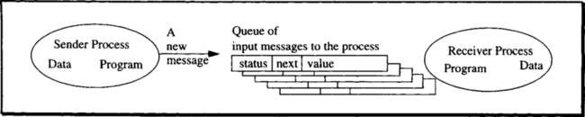
Message delivery is not reliable. Some messages are lost (they are never delivered). Some may be delayed, arbitrarily permuting the message delivery order to a process’s input queue. Even if a message is delivered, there is some small chance it will be corrupted, so that the message data is unreadable. The loss and corruption of messages is quantified as the probability of message failure, pmf. There is a comparable chance that the message will be duplicated, so that the message appears twice in the process’s input queue. The following example code demonstrates the external definition of message gets and sends.
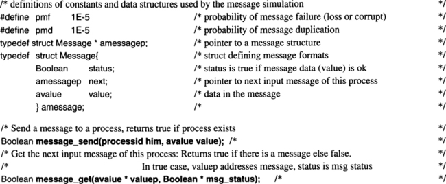
The next piece of code gives a sense of how these routines are used, and it defines a useful routine. This get_msg() routine discards corrupt input messages and returns false if there are no good new messages in the process input queue, or returns true and the data of the next input message.

This completes our brief overview of messages. Messages are explored further in Subsection 3.7.4, following the introduction of reliable processes.
3.7.3.2 Process Fault Model
A process executes a program, transforms the process state, and displays an execution behavior. The process’s external behavior is a sequence of store_read(), store_write(), message_send(), and message_get() operations. This external behavior is created by the process executing its program logic on the process state. Each process state is a bundle of bytes containing its program and data. Each process has two states, an initial state that never changes and a current state that changes at each program step. In addition, each process has an input queue, an unordered set of messages sent to it by other processes.

A process fails by stopping for a while (say, an hour) to be repaired, then being reset to its initial state, and having all its unprocessed input messages discarded. That is analogous to a restart of processors in many operating systems. At any instant, each process runs the risk of faulting. After a reset, the process executes its restart logic and continues processing. Of course, it runs the risk of experiencing another reset during the restart.
Here is a way to think of process faults: Imagine that each process is implemented by a lower-level automaton that usually executes the next step of the process, but sometimes stops the process execution for a repair period, discards all the process’ messages, resets the process to the initial state, and then continues the process execution from the initial state (this state includes the process’ program). In addition, the process may have defensive programming tests that cause it to failfast by calling panic() if the test is false. These calls to panic are modeled as just another aspect of the execution automaton occasionally failing the process. Such an automaton is defined as follows:

3.7.3.3 Reliable Processes via Checkpoint-Restart
So far, the processes described are failfast: they either execute the next step, or they fail and reset to the null state. They are not reliable because they do not repair their state upon failure. This failure behavior is similar to the storage failure model in which stores return to service in the null state. Some mechanism is needed to repair the process state, that is, to bring it up to its most recent value.
There are many ways to build such reliable processes from failfast processes. For simplicity, assume that every process’ state fits within a single page. It is then easy to generalize to larger processes.
The following discussion proceeds by example, showing three different ways to implement the same server process. The server’s job is to return a unique sequence number, called here a ticket, to each client upon request. It must never return the same ticket number to two different client requests. Clearly, to achieve this the server must reliably remember the most recently granted ticket number.
The simplest design is the checkpoint-restart approach. The process keeps two copies of its state in reliable storage. At each state change, it overwrites the oldest state value (ticket number) in reliable storage. At restart, it reads both state values and resumes execution from the most recent one (see Figure 3.19). The following code gives a simple example of a reliable checkpoint-restart process.


Checkpoint-restart is a classic technique that has been widely used for decades (see Figure 3.1). Its major problem is that the repair time for the process can be quite long, since the process does not resume service until it is started and refreshes its state from persistent storage. The total repair time is therefore the process repair time plus the restart time, which, according to the model, is several hours altogether.
Because of the long repair times, checkpoint-restart yields highly reliable process execution, but not highly available process execution. The goal is to continue the process execution immediately after the process faults, meaning instant (almost zero) MTTR of process faults. If the fault is caused by hardware, it is likely that pair-and-spare hardware or triplexed hardware can mask it. If the fault is caused by software, by operations, or by environment (as most faults are), then the process and processors will fault, and the process will stop. Why not have a second process in a second processor take over from the first if the first process fails? That idea, called process pairs, is the next technique.
3.7.3.4 Reliable and Available Processes via Process Pairs
The process pair technique is somewhat analogous to n-plexed storage; it is a collection of n processes dedicated to providing a service. One of the processes is primary at any time. The primary process delivers the service. If the primary fails, the backup process continues the service. Clients send their requests to the primary, and if the primary fails, the new primary informs the clients of its new role.9
The two-process case, process pairs, is subtle enough. It allows a second process to take over from the primary. There are two delicate aspects of takeover:
As with all aspects of fault tolerance, detecting the primary failure is purely statistical. Because the primary can send messages only when it is operating, a failed primary cannot inform the backup that the primary is broken. For this reason, the primary sends I’m Alive messages to the backup on a regular basis. If one I’m Alive message fails to arrive on time, it is assumed to be delayed or damaged. But if several I’m Alive messages fail to arrive within a reasonable time, the backup assumes that the primary did not send them and is being repaired.
Suppose the backup has decided that the primary is dead. What should it do? How can it continue the computation from the most recent primary state? First, it needs to know the most recent primary state. The usual technique is for the primary to combine state-change messages to the backup with the I’m Alive messages, so-called checkpoint messages. For example, in Figure 3.20 the I’m Alive messages are being sent frequently to the backup. Clearly, the state-change messages can piggyback on the I’m Alive messages, or they can act as surrogates for them. The basic logic of a process-pair program is shown in Figure 3.21.


The idea presented in Figure 3.21 is that both processes start out in the restart state. One process (say, the even-numbered one) is the default primary and takes priority by waiting only one second to see if the other is alive. After two seconds, either the default primary process will have generated an I’m Alive message to the default backup, or the backup decides the primary is dead. In that case, the backup becomes the primary. In any case, whichever becomes the primary broadcasts its identity to all concerned and then goes into a loop of looking for input and processing it. This loop continuously sends I’m Alive messages to the backup, whether there is any input or not. For its part, the backup sleeps for a second, looks to see what the new state is, and then goes back to sleep. The “newer state” test is designed to avoid the possible permutation of messages in the input queue by ignoring states older than the current backup’s state. This test also discards duplicate messages. If the backup does not get a new state within a second, then the primary must be dead, since the primary ought to be able to send hundreds of I’m Alive messages in that time. If the primary is dead, the backup broadcasts that it is the new primary and waits for requests.
There is one more delicate takeover issue. At takeover, the backup is in the same state the primary was in when it sent the checkpoint message to the backup. But the primary may have failed before sending the reply that the last state transition generated (the bottom box of Figure 3.21). So, if a reply was owed to a client, the reply is resent. This may generate a duplicate message to the client, but that was a possibility of the message system anyway.
To continue the discussion of Figure 3.21: If the maximum propagation time for messages is one millisecond, and the maximum service time for a request is a millisecond, then waiting ten milliseconds (five message cycles) is long enough to detect process failure. This period is long enough for five consecutive lost I’m Alive messages if processors are dedicated to processes. Thus, process takeover times of ten milliseconds can easily be achieved. Typically, though, the primary shares the processor with other processes and, for resource consumption reasons, does not continuously send I’m Alive messages. Consequently, a longer latency is more typical.
In fault-tolerant operating systems, process pairs are a basic notion provided by the system. Such operating systems inform the backup process when the primary process fails and automatically redirect all new client requests to the backup process. This means that the primary can dispense with the idle state checkpoint messages and the I’m Alive messages. It also means that the backup can dispense with the one-second waits, because all the messages are important. The backup can also dispense with the broadcast to clients at startup and takeover. These are just performance optimizations; the programming style of checkpointing state changes is the same for this simple model and for the “real” fault-tolerant systems.
Adapting the checkpoint_restart_process() example to process_pair_process() using the logic of Figure 3.21 is straightforward (about one page of C code). The complexity of process pairs apparent in the above explains why the discussion here is restricted to process pairs, rather than including n-plexed processes.
3.7.3.5 The Finer Points of Process-Pair Takeover
No known technique continues process execution immediately after a fault.10 The known techniques offer takeover times on the order of a few message propagation delays. In a cluster or local network, this takeover can happen in milliseconds when software overheads are considered; in long-haul nets, the message propagation delays imply that takeover times will be on the order of tens or hundreds of milliseconds (see Section 2.9 for a discussion of message propagation times). To clients operating on a time scale of seconds, this takeover may appear immediate. Certainly, it is a big improvement over the availability offered by the checkpoint-restart approach, which has outages measured in minutes or hours.
There are a few additional details. If state-change checkpoint messages were permuted in the backup process’ input queue, then an old state might replace a newer one. The permuted messages problem is easily solved by having the primary process sequence number the state-change messages, and by having the backup ignore old ones—ones with sequence numbers less than the current sequence number. The next problem is much more serious. If the checkpoint messages are lost and the primary fails, then the backup will not be in the correct state. At this point, one must appeal to the single-fault tolerance assumption. These are process pairs; they tolerate single faults. If both a process and the message fail, then there is a double failure, which is not protected. Assuming independence of failures, the mean time to such failures is approximately MTTPF/pmf, the time to a process failure over the chance that the most recent message was lost. For the numbers chosen in the process and message model above, that is (≈ (107/10−5) = 1012)seconds, or about thirty-thousand years. If that answer is not acceptable, then a safer approach is to have the backup acknowledge receipt of the state change before the primary responds to the client. But now the primary has to sense backup failures (it has to know when to stop waiting for the backup to acknowledge). This acknowledged-checkpoint strategy is the one used in the Tandem Computer’s process pairs; for the sake of simplicity, however, it is not the one described here.
The ticket-number generator program was used to demonstrate checkpoint-restart logic. This three-line program is not very demanding, either as a checkpoint-restart process or as a process pair. Its only requirement is that it never generate the same ticket number twice. As such, it fails to expose one of the most delicate issues in takeover. Suppose the primary is performing some real operation, such as advancing the rods in a nuclear reactor by one inch, and then it fails. The backup may be in a quandary: did the primary perform the operation or not? The backup cannot tell unless it “looks” at the rods. Sometimes, though, it is not possible to “look.”
A whole vocabulary has been built up around this problem. First, an operation is testable if the program can reliably establish whether the operation has been performed and the desired effect achieved. Writing pages to disk is testable (they can be read to see if they have changed). Moving reactor arms to a particular position is testable, but movement to a relative position is not: “move to position X is testable,” while “move 1 inch” is not testable. Writing to a display or printing on paper is not testable. In general, many physical operations are not testable. The safe thing, then, is to redo the operation: move the reactor arm to position X again, write to the display again, print the message again, and write to the disk again. But not all operations can safely be redone. An operation is restartable or idempotent if redoing it is safe; that is, if redoing it an arbitrary number of times is equivalent to doing it once. Moving the reactor rods one inch is not restartable, printing a check is not restartable (n operations are likely to print n checks), and inserting a record at the end of a file is not restartable (it may insert the record n times); but moving the rods to position X, writing a disk page, and writing a display are probably idempotent operations.
In Figure 3.21, resending the reply message at takeover is trying to deal with the idempotence issue. The takeover process cannot tell whether the client received the reply to his request, so the server resends the reply on the premise that the message will be discarded by the client if it is a duplicate. The operation is not testable, but it is assumed to be idempotent.
3.7.3.6 Persistent Processes—The Taming of Process Pairs
As can be seen from the previous discussion, writing process pairs is very demanding. Indeed, it is the authors’ experience that everyone who has written one thinks it is the most complex and subtle program they have ever written. However, reliable systems use these techniques, and those systems do mask many failures.
There is a particularly simple form of process pair called a persistent process pair. Persistent process pairs have a property that is variously called context free, stateless, or connectionless. Persistent processes are almost always in their initial state. They perform server functions, then reply to the client and return to their initial state. The primary of the persistent process pair does not checkpoint or send I’m Alive messages, but just acts like an ordinary server process. If the primary process fails in any way, the backup takes over in the initial state.
Persistent process pair takeover works as follows. The underlying fault-tolerant operating system knows that the primary and backup are a process pair. If the primary fails, or if the processor on which the primary is executing fails, the operating system of the backup process senses the failure and informs the backup process of the failure. The operating system also redirects all client messages to the backup. In this situation, the backup takes over in its initial state and begins offering service.
As described, persistent processes are easy to program and make high-availability servers, but these servers seem to provide little more than encapsulation of the server logic to the client. The servers do not maintain network state or database state. To make persistent processes useful, someone else must maintain such states.
For example, imagine that such a persistent process acted as your mailbox. It would receive messages for you, but would always return to the null state (no messages for you)—not a very useful program. Similarly, if the server actually kept your state in a file, the updates to receive or discard a mail message might be partially incomplete at the time the server failed. In this case, your mailbox file would be left in that state by the backup persistent process when it took over in the null state.
These examples hint at the solution. A persistent process server should maintain its state in some form of transactional storage: a transaction-protected database. When the primary process fails, the transaction mechanism should abort the primary’s transaction, and the backup should start with a consistent state. On the other hand, if the server calls commit_work() after making the changes, the transaction mechanism should reliably deliver the server’s message to the client as part of the atomicity guarantee of ACID transactions.
Given that, the transaction mechanism returns the database and the network to their state as of the start of the server function. Persistent processes need not send application checkpoint messages to indicate state changes, since the initial state is the takeover state. When running on a fault-tolerant system that provides persistent process pairs as a primitive, the program need not concern itself with takeover or message retransmission. That logic is handled for the program by the underlying system. All this makes persistent process pairs very easy to program. They have the following form:

The following code illustrates the checkpoint-restart ticket server of Subsection 3.7.3.3 reprogrammed as a transactional server.

Notice that to become a process pair, the ticket server application did nothing more than represent its state in transactional storage and call the operating system routine wait_to_be_primary(). There are no checkpoint messages, no I’m Alive messages, and no takeover logic. Yet this process has much higher availability than the checkpoint-restart process. In addition, if the transaction did complex updates to its database, each group of updates (transactions) would have all the ACID properties.
3.7.3.7 Reliable Processes plus Transactions Make Available Processes
Transactions provide highly reliable execution, but ACID says nothing about availability. All the ACID properties are reliability properties. Process pairs provide highly available execution (processes), but they are hard to program because takeover is so delicate. The transaction ACID properties provide clean takeover states: transactions combined with persistent process pairs give both high reliability and high availability by allowing simple programs to use process pairs.
Virtually all fault-tolerant application-level process pairs are now programmed as persistent processes. Only low-level processes (device drivers, disk servers, TP monitors, and the transaction mechanism itself) are programmed as raw process pairs. These more basic processes cannot use the persistent process approach, primarily because they are below the level of abstraction that provides the high-level process-pair and transaction mechanisms.
Highly available systems contain many process pairs. The storage repair processes mentioned previously need to be process pairs. If the storage is shared and access to it must be serialized, then the storage servers should be process pairs. If reliable storage is to be implemented, then the reliable writes should indeed be reliable (write all n of the n-plex). To protect against faults within the reliable write code, it should be run as a process pair, and so on.
Process pairs depend critically on the premise of single failure (only one processor fails) during the repair period. If the pair of processes has a shared power supply (or shared memory or any other single point of failure that can disable them both), then this assumption is violated. The processes must therefore be connected to each other, to their storage, and to their clients via dual networks. They must have independent power supplies and, of course, they must have different processors and memories. In addition, each component should have independent failure modes and be failfast. It is fair to say that today most hardware systems are not constructed to meet these demands. Several attempts to build process-pair systems have failed. Yet there are two successful examples, Tandem’s Guardian system and IBM’s XRF system. The XRF design demonstrates that it is possible to retrofit these ideas to a preexisting general-purpose transaction processing system (IMS in this case).
In summary, given failfast processes that fail independently, there are two ways to get highly reliable processes (checkpoint to storage or checkpoint to a backup process) and one way to get available processes (process pairs). The model allows us to talk about and analyze both.
3.7.4 Reliable Messages via Sessions and Process Pairs
Having shown how to convert faulty processes and faulty storage to highly available processes and storage, the discussion turns to converting faulty messages to highly reliable messages. This section first defines the behavior and fault model for messages. It then shows how sessions, session sequence numbers, acknowledgment, timeout, and retransmission can all be combined to provide reliable message delivery. Since either the message source process or the destination process can fail, process pairs are part of the mechanism needed to convert faulty messages into reliable messages.
3.7.4.1 Basic Message Model
A process can send a message to another process by invoking message_send(), which specifies the process identifier and the message data. This copies the message data from the sender’s address space to the receiver’s input queue. The receiver can then call message_get() to copy the message from its input queue to its address space.
The message and process queue definitions were already given. Here is the code to implement message_send and message_get:

Messages have simple failure modes; some fraction of them spontaneously decay (status = FALSE) and some fraction of them are duplicated. This models failure of communication lines, buffer overflows, and the like. It also models the retransmission logic underlying message systems that occasionally duplicate a message. In addition, the messages in a process’s input queue may be arbitrarily permuted. This models the possibility that messages can be arbitrarily delayed in the network.
3.7.4.2 Sessions Make Messages Failfast
As defined, messages are not failfast; corrupt and duplicate messages are delivered, and messages are delivered out of order. The first step in making messages reliable is to give them simple failure semantics—failfast semantics. To make all messages failfast, faulty messages are converted to lost messages. Message semantics, then, are as follows: (1) messages are delivered in order, and (2) some messages are lost. In the simplified model, the only form of message failure is a lost message.
First, let’s convert corrupt messages to lost messages. The message status flag models the idea that the message contents are self-checking, so that corrupt messages can be detected and discarded. It is standard to compute a message checksum at the source and to send the checksum as part of the message. The receiver recomputes the checksum and compares it to the sender’s checksum. If the two checksums are different, the message has been corrupted and is discarded. This converts a corrupt message to a lost message. The get_msg() procedure defined in Subsection 3.7.3.1 discards all such corrupt messages.
The simplest approach to detecting and discarding duplicate and permuted messages is to use sessions and message-sequence numbers. A session is a bidirectional message pipe between two processes. Sessions have the following semantics: (1) messages are delivered to the destination in the order they were sent, and (2) no messages are duplicated or lost, but messages can be delayed. Sessions are variously called connections, sockets, pipes, dialogs, opens, ports, and myriad other names. In this text, sessions are represented by pipe icons, as shown in Figure 3.22.

Sessions implement these semantics by having the two session endpoints each maintain three sequence numbers: (1) the out sequence number, which is the sequence number of the most recently sent message on that session, (2) the in sequence number, which is the sequence number of the most recently received message on that session, and (3) the acknowledged sequence number, which is the sequence number of the most recently acknowledged message.
Each message from one process to another carries a sequence number. When a new message is sent to that receiver, the sender’s out sequence number is incremented and used to tag the sender’s message. When the receiver gets the message, if the sequence number is one greater than the most recent message, the recipient knows it is the next message and accepts it. The recipient increments the in sequence number and sends an (unsequenced) acknowledgment message to the sender, saying that the new message arrived.
Sequence numbers detect duplicate and delayed messages as follows: If a message is duplicated, the message sequence number is also duplicated; thus the recipient can detect a duplicate message by noticing that the message sequence number is equal to the most recently acknowledged sequence number. In this case, the recipient discards the message and does not change its in sequence number. In either case, the recipient acknowledges the message to the sender.
If a message is delayed and hence arrives out of order, the recipient can see that the message sequence number is less than the most recently acknowledged message and consequently can discard the message. It need not acknowledge such messages.
As described so far, sessions create the simple failure semantics of sending messages in order, thereby making messages failfast. If there were no failures, such sessions would work perfectly. But, as soon as there is a message failure, the session starts discarding all future messages in that direction. So far, then, the design has made messages failfast. The next step is to make messages reliable by repairing lost messages.
3.7.4.3 Sessions plus Retransmission Make Messages Reliable
To restate the session message-sending protocol: When one process sends a message to another, the sender increments the session out sequence number and tags the message with the session name (the names of the two processes) and the sender’s current out session sequence number. The sending process then waits for an acknowledgment message, called an ack, from the recipient. The ack message carries the session name and the original message sequence number. Because message failures cause messages to be lost, the acknowledgment may never arrive. In such cases, the sender must resend the message.
To repair lost messages, the sender has a timeout period. If the sender does not receive an ack within a timeout period, it retransmits the message and continues to do so until an ack is received. If the sender and receiver are functioning, the message eventually is delivered, and the ack is delivered. When that happens, the sender declares the message delivered and increments its acknowledged sequence number.
3.7.4.4 Sessions plus Process Pairs Make Messages Available
The discussion so far has focused on message failures and ignored process failures. What if the sending or receiving process fails? In that case, the message has nowhere to go or no sender to retransmit it. A session is only as reliable as its two endpoints.
The obvious solution to making reliable session endpoints is to make each endpoint a process pair. In this design, sessions connect process pairs so that delivery of new messages to the backup is automatic if the primary fails. Messages that have already been sent to the primary are probably lost and will not arrive at the backup. The sequence numbers of the primary are also maintained as part of the backup process state. If a process fails, that endpoint of the session switches to the backup of that process pair. The backup will have the current sequence numbers, and if it is sending, it will have a copy of the current message.
The logic for this is simple: The sender first checkpoints the message to the backup and then sends the message. If the backup takes over, it resends the message and continues the session. The receiver checkpoints received messages to its backup before acknowledging them. This logic is diagramed in Figure 3.23.

At process-pair takeover, the backup process broadcasts its new identity and resends any unacknowledged messages that the primary process was trying to send. The other session endpoint may get a takeover broadcast from the backup process of the process pair. In that case, the other endpoint begins sending the message to the former backup process, which is now the new primary process of the process pair. When the message is finally delivered and acknowledged, the next message can be sent via the session.
To restate this development: Session sequence numbers convert permuted messages and duplicate messages into lost messages, making all messages failfast and making sessions failfast-communications services. Acknowledgment, timeout, and retransmission make messages reliable by resending them. Messages eventually get through. Process pairs make the endpoints available; they are persistent in sending the messages until they are acknowledged. Messages are as available as the processes that send them and the wires that carry them. If the processes are duplexed, and the wires are n-plexed, the messages can be made highly available. The various time constants (acknowledge times and takeover times) are limited by message delay and processor speed. It is possible to give reliable delivery within seconds for wide-area systems (≈10,000 km) and within tens of milliseconds for local area systems (1 km). These time constants are discussed in Section 2.6.
3.7.4.5 The Code for Sessions and Messages
The code to implement sessions, acknowledgment and retransmission, and process-pair checkpoint and takeover is instructive. First, sessions and message formats are defined, and an array of sessions is added to the state of each process. These sessions hold the endpoint names and the sequence numbers.

In addition, assume that the message_send() and message_get() routines have been abstracted to session_send() and session_get() routines. These routines send and get messages that carry a session descriptor and a message type (that is, they manipulate the a_session_message type rather than just a_message type). These routines pack and unpack the session descriptor and message type descriptor as added framing information on messages. Session_send() fills in the session descriptor and value for each message. Session_get() extracts these two fields from the next process input message and returns them. Session_get() must read the message to find the session name and the sequence number. If the message is corrupt (status = FALSE), session_get() cannot read these fields and discards such messages. Consequently, it has no status parameter; any message it returns is not corrupt. These are the interfaces:

The reliable_send_message() routine sends the message, waits for the timeout period, and if no acknowledgment message has arrived, it sends the message again. It continues this until the message has been acknowledged (the acknowledgment mechanism is explained momentarily):

In this design, the sender continues sending until the receiver acknowledges the message. The receiver may be doing something else at the moment—computing, writing storage, or even sending a message to some third process. The receiver, therefore, may not be interested in acknowledging the sender’s message right away. Waiting for the receiver’s acknowledgment might cause message deadlock, with each process waiting for an acknowledgment from the next. To avoid such deadlocks, and to speed message flows, acknowledgments should be generated quickly and asynchronously from the receiver’s application program logic. This means that each process should regularly poll its input sessions for messages. Such a requirement, however, would make programs both unreadable and error-prone.
Even more fundamental, perhaps, is the fact that the sender in the code above assumes someone else is going to update the acknowledgment sequence number. The reliable_send_message() code could perform this logic, but it would vastly complicate the code. In general, this is the kind of logic that another process should manage as a service for all processes in the address space.
To preserve the program structure, almost all systems use the concept of multiple processes sharing one address space to perform such asynchronous tasks (see Chapter 2). Such lightweight processes are often called threads, but the generic term process is used here. These processes execute continuously and autonomously from the main application, communicating with it primarily via shared memory. The main application function is implemented as one or more processes (threads), and service functions such as message acknowledgment are implemented as other processes.
Each address space has a listener process that performs message acknowledgment and increments message sequence numbers for the application process executing in that address space. The listener is constantly polling the application process’s sessions. When a message arrives, the listener executes the sequence number logic. If the message is a data input message, the listener acknowledges the message and places it in the session’s message queue for the application program process. If the message is an acknowledgment, the listener implements the ack sequence number logic. Figure 3.24 illustrates the role of the listener.

The listener process executes continuously, running at high priority. When there are no input messages, it waits for the next event (in the sample code it waits for a second rather than for an event). In most designs, the listener places a limit on how many messages it will accept from a sender. This is called flow-control. Otherwise, senders could flood the receiver with messages, consuming all the listener’s storage. For simplicity, such refinements are not included in the example. Also for simplicity, the code does not deal with takeover (process pairs). The listener maintains the process sequence numbers and the FIFO session message queues.

The picture thus far is that the listener acknowledges receipt of messages promptly and saves these messages as part of the process (pair) state. The acknowledged input messages of each session are chained from the in_msg_queue[] of that session in most-recent-last order. It should now be clear that reliable_send_message() does reliably send messages. It retransmits every second until the message is acknowledged and the listener records that acknowledgment by incrementing the session.ack sequence number.11
Reliable_get_message() gets the next message value from a particular session by accessing the message queue maintained by the listener. The code to reliably get a message follows:
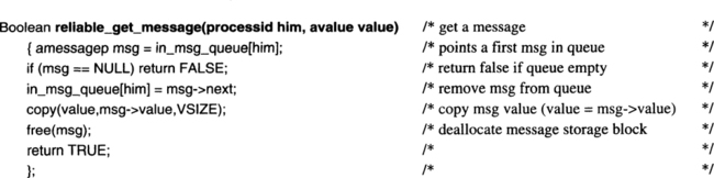
3.7.4.6 Summary of Messages
Reliable_get_message() and reliable_send_message(), combined with the listener process, convert ordinary messages into failfast messages. They discard corrupt messages, duplicates, and permutations. Sender timeout and retransmission until acknowledgment transform fail-fast messages into reliable messages. Process pairs make the session endpoints available, thereby transforming reliable messages into highly available messages. This sequence of steps shows how ordinary unreliable messages can be transformed into a reliable and available message service.
Fault-tolerant operating systems provide the reliable message get and send logic, the listener logic, and the logic to redirect messages to the backup of a process pair at takeover. For this reason, most application programmers are unaware of the acknowledgment-timeout-retransmission issues; they are even unaware of the checkpointing of the message sends and acknowledgments to the backup. But it is useful to have this simple model of how the underlying message system works.
One nice way to talk about messages is to say that raw messages may be delivered zero or more times. By adding sequence numbers and discarding duplicates, messages are delivered at most once. Such messages, however, may be delivered once or not at all. By adding retransmission, messages are delivered to a process exactly once. But this just means the message was delivered to the listener. Perhaps the message was never delivered to the application, or was never acted upon by the receiver. By adding process pairs, the message is processed exactly once. Consequently, these techniques give a simple form of message atomicity and durability (the A and D of ACID).
3.7.5 Summary of the Process-Message-Storage Model
The preceding gives a simple simulation model of the three components of a computer system. The message and storage models show how software can mask hardware faults by using redundancy in hardware, duplexing storage, wires, and processors. It also shows how software can use redundancy in time by retransmitting a message if the first one fails.
This material gives a sense of three styles of software fault tolerance: checkpoint-restart, process pairs, and persistent processes. It also gives a sense of the relative difficulty and benefits of the three styles, with the goal of convincing the reader that, if possible, persistent processes plus transactions should be used to obtain highly available program execution.
In addition, this simplified model (leave aside the actual implementation) is fairly complex. No formal or theoretical development of these ideas is available—it would be too difficult and complex to handle. In contrast, the model might work well for simulation studies to help quantify the relative benefits of design alternatives.
3.8 General Principles
We have all learned the following two rules, and done so by bitter experience:
Murphy. Whatever can go wrong will go wrong at the worst possible time and in the worst possible way.
Modularity, failfast, n-plexing, and ACID are all attempts to deal with these rules. Imagine programming a module that either works or misbehaves arbitrarily, and trying to tolerate the arbitrary misbehavior. That is the behavior predicted by Murphy’s law. Failfast, also called all-or-nothing (atomicity), simplifies failure modes. Simplicity is what KISS is about. Don’t be fooled by the many books on complexity or by the many complex and arcane algorithms you find in this book and elsewhere. Although there are no textbooks on simplicity, simple systems work and complex ones don’t. Modularity, failfast, n-plexing, and ACID are mechanisms that simplify design, and make it easier to build systems with high functionality yet simple structure.
Given that things fail, and given that they fail fast, then repair is important to both reliability and availability. Process pairs, disk pairs, system pairs, and quick message retransmission all yield repair times measured in milliseconds—in effect, instant repair for people and physical processes that operate on time scales of seconds.
If faults are independent, then single-fault tolerance, combined with repair, yields MTTFs measured in decades or millennia. At these rates, other factors become significant (labor disputes, fires, floods, business panics, or whatever). The next improvement is several orders of magnitude away and is justified only rarely, generally only when human life is at stake.
Designing a fault-tolerant system needs a model of fault modes and their frequencies. The hardware and software design should minimize module interdependencies to get good fault containment. If faults are to be independent, the modules should have independent failure modes—suspenders and a belt, rather than two pairs of suspenders or two belts. This is sometimes called design diversity.
A model of fault tolerance needs to be end-to-end. It needs to look at the whole system, including operations and environment, to make estimates of system reliability and availability and to tolerate faults at the highest level of abstraction. The next section has an extended example of end-to-end problems.
The models used in the previous three sections are not end-to-end: They focus on the narrow topics of hardware or software fault tolerance. But they do allow careful discussion of the key fault-tolerance architectural issues. The message model and storage model of the previous section are relatively easy to understand and use. In contrast, the process pair model is intellectually challenging for the brightest people. As such, process pairs are a dangerous tool. Transactions combined with persistent process pairs are a solution. They provide simple process pairs (persistent execution) and a simple fault model.
In the limit, all faults are software faults—software is responsible for masking all the other faults. The best idea is to write perfect programs, but that seems infeasible. The next-best idea is to tolerate imperfect programs. The combination of failfast, transactions, and system pairs or process pairs seems to tolerate many transient software faults.
3.9 A Cautionary Tale—System Delusion
The focus here on system failures ignores the common end-to-end problem of system delusion: The computer system and its communications and terminals are up, but the output is untrustworthy or useless because the database is inconsistent with reality. System delusion generally results from incorrect transactions and from unrecorded real-world activities.
A specific example of system delusion may help in understanding the problem. Company X built an elaborate system to optimize and control the inventory of spare parts used for repairs. The application tracks many field locations, each with various types of inuse parts and spare parts. It also tracks a few central stock locations where parts ordered from manufacturers are stored until they are needed in the field. The stock locations also receive from field sites any unneeded spares and any defective parts that require repair. In principle, each field location does a transaction any time it uses a part or removes it from use, and a transaction each time it needs parts from central stock or returns parts to central stock. A central administrator runs transactions to release parts from central stock to the field, to order more parts from vendors, to record their receipt, and so on. As stated, this is a classic inventory-control problem.
As it turns out, the big problem with this system is not system failures. These do occur, but they are minor compared to the difficulties caused by unrecorded activities and by incorrect transactions.
Unrecorded real-world activities were a problem for various reasons. For example, optimal spare stocking levels are not intuitively obvious to people in the field. Most field managers gradually acquired extra spares, beyond what a reasonable inventory manager would agree was needed. Exactly how the field managers did this wasn’t entirely clear, but they did it. Then, every once in a while they would get tired of seeing spares sitting around gathering dust and would dump the excess into cartons and send it back to central stock, but without any indication of where it was sent from (this to avoid admitting they had the stuff in the first place). Such activities guaranteed that the transaction system was constantly out of touch with reality, which made inventory management remarkably difficult. In particular, the spare reorder process tended to be seriously unstable.
This problem was eventually solved by adding heuristics to detect locations reporting activities inconsistent with recorded stocks. These tests triggered a physical reinventory of those sites. Even that was an art. For example, the field managers routinely hid excess inventory in the women’s rest rooms.
Another example demonstrates the difficulties caused by incorrect transactions. An improperly trained clerk, told to change the accounting classification of a very large number of parts, spent two weeks deleting these parts from the database. When this was discovered, it was impossible to just roll forward from two weeks ago because, although database backups and log tapes were available, the incorrect deletions had caused various other things to happen that had real-world consequences. Complicating the situation, the deletions had caused the deleted part descriptions to disappear entirely from the on-line database (in hindsight, a serious flaw in application design). So, several people spent a month going back through the journal tapes looking for and recreating the deleted modules. Meanwhile, nobody really trusted the output of the transaction system; as a result, a lot more people spent time manually reviewing transactions.
The point of these two stories is that a transaction system is part of a larger closed-loop system that includes people, procedures, training, organization, and physical inventory, as well as the computing system. Transaction processing systems have a stable region; so long as the discrepancy between the real world and the system is smaller than some threshold, discrepancies get corrected quickly enough to compensate for the occurrence of new errors. However, if anything happens (as in the case of the improperly trained clerk) to push the system out of its stable zone, the system does not restore itself to a stable state; instead, its delusion is further amplified, because no one trusts the system and, consequently, no one has an incentive to fix it. If this delusion process proceeds unchecked, the system will fail, even though the computerized part of it is up and operating.
More generally, this is an end-to-end argument. Most transaction processing systems are vulnerable to failure by getting out of touch with reality. System delusion doesn’t happen often, but when it does there is no easy or automatic restart. Thus, to the customer, fault tolerance in the transaction system is part of a larger fault-tolerance issue: How can one design the entire system, including the parts outside the computer, so that the whole system is fault tolerant? This may involve such exotic things as finding heuristics that detect transactions and data patterns that are seriously out of touch with reality. System designers must consider such organizational and operational issues as part of the overall system design.
3.10 Summary
The first section of this chapter reviewed empirical studies of computer systems and showed that the major sources of failure are environment, software, and operations. Hardware, maintenance, and process are relatively minor failure sources today, and the trend is for them to become even more reliable.
The next section described how hardware designers do it: they use either pair-and-spare or TMR to get failfast modules with instant mean time to repair of a single fault. Repair was shown to be a critical part of the design.
The discussion then turned to software, exploring two approaches: n-version programming and transactions. Both schemes try to mask transient software failures. It was shown that n-version programming without repair is of questionable value.
Next, a more detailed software fault masking view was explored. Simple fault models for processes, storage, and messages were defined. These unreliable entities are first transformed into failfast stores, processes, and messages. Then they are transformed into reliable and available entities. N-plexing of storage with a version number for each logical page provides highly available storage. Sequence numbers, acknowledgment, timeout, and retransmission provide reliable messages, and process pairs provide highly available execution. Process pairs are needed to ensure that messages are delivered reliably and that replicated storage groups are updated reliably. These concepts are the basis for understanding the algorithms used in “real” fault-tolerant systems.
At a low level, hardware designers must deal with pair-and-spare or TMR, and software gurus must deal with process pairs. Fortunately, most of us are handed this substructure and even a transaction processing system built on top of it. Given these, we can build applications and subsystems using ACID transactions, persistent processes, system pairs, reliable messages, and reliable storage. Mid-level software—such as database systems, compilers, repositories, operator interfaces, performance monitors, and so on—can all be written atop this base as “ordinary” applications. The transaction mechanism with failfast hardware and instant repair can then mask most systems programming faults, most application programming faults, most environmental faults, and most operations faults.
The chapter concluded with some free design advice: keep it simple and worry about end-to-end issues. To drive home the end-to-end point, an extended example of system delusion was described—a system that was “up” but was completely out of touch with reality because it did not tolerate faults in the organization it served.
3.11 Historical Notes
Fault tolerance has been important since the inception of computers, and there have been an enormous number of contributors to the field. Von Neumann’s early work is generally cited as the beginning, but Charles Babbage mentioned the need for redundancy. Of course, auditors have been performing duplicate calculations and keeping multiple copies of things for millennia. Error detection and correction has been a key part of data transmission for many decades.
The empirical measurements are based on Eiichi Watanabe’s translation of a study done by the Japanese. In addition, we benefited from the work of Ed McClusky’s students at Stanford in the mid 1980s [Mourad 1985], and from Ed Adams’s study of IBM software faults [Adams 1984]. Many people, who wish to remain anonymous, gave us statistics on the availability of their (or their competitors’) systems. Those statistics are encrypted within this chapter.
Disk duplexing was widespread soon after disks were invented; disks were very unreliable at first, making duplexing essential. As disks became more reliable, duplexing became more exotic, but it had a rebirth as disks got cheaper.
The ideas for failfast, pair-and-spare, and TMR were worked out by the telephone companies, the military, and the deep-space missions. The book by Avizienis [1987] gives a good survey of those developments. Avizienis’ later study [1989] and Abbot [1990] do a good job of reviewing work on n-version programming. The seminal text on fault-tolerant computing by Dan Siewiorek and Robert Swarz [1982] contains a wealth of information. Section 3.5 borrows heavily from their analysis of availability and reliability. The tutorial by Flaviu Cristian [1991] gives a good summary of current work in fault-tolerant systems from a software perspective. Bruce Lindsay is credited with coining the term Heisenbug.
The ideas for process pairs have deep roots as well. The presentation in this chapter draws heavily from the process-pair design of Joel Bartlett in Tandem’s Guardian operating system done in 1974, and from the Lampson and Sturgis paper [1976]. Alsberg and Day [1976] had similar ideas in that era, but seem not to have developed them. The model of storage and messages is based on the Lampson-Sturgis model [Lampson 1979 and Lampson 1981].
The ideas for system pairs also go back a long way. Many such systems have been built since 1960. General-purpose systems are just beginning to emerge. The first organized approach to this problem was SDD-1. Typical reports describing that system are Bernstein and Goodman [1984] or Hammer [1980]. Notable commercial systems are IBM’s XRF [IBM-IMS-XRF] and Tandem’s RDF [Tandem-XRF]. Intensive research on this topic is proceeding at Princeton [Garcia-Molina 1990], IBM Research [Burkes 1990], and Tandem [Lyon 1990].
The taxonomy of at least once, at most once, and exactly once message semantics is due to Alfred Spector. The concept of the testability of an operation is due to Randy Pausch [1987].
Exercises
1. [3.1, 10]. This exercise is designed to get you thinking about failure rates. Suppose you are 20 years old and you learn that one 20-year old in a thousand will die this year. (a) What is your mean time to failure? (b) What is your failure rate per hour? (c) If there are 100 people in your class, all the same age, what is the chance one of them will die this year? (d) Why is the answer to question (a) so much higher than your life expectancy? (e) Is this failure rate memoryless on the time scale of weeks and on the time scale of decades?
2. [3.1, 20]. Even though the mean time to failure of a module is one year, a module may operate for many years without any failure. The probability of a failure within a certain time may be estimated as follows: The arrival rate of failures is λ = 1/mttf. Suppose, as is often done, that failure rates obey the standard negative exponential distribution that has the formula f(t) = λ • e−λt. Then the chance of not failing between now and time T is the integral of this function

Returning to the original example, what is the chance of failing within .5 year, within 1 year, within 2 years, and within 10 years?
3. [3.1, 10]. Suppose your car has four failure modes with the following mean times to failure: wreck: 20 years, mechanical: 1 year, electrical: 3 years, flat tire: 3 years, and out-of-gas: 3 years. (a) What is the mean time to failure of the car? (b) How much better would it be if you never ran out of gas?
4. [3.1, 10]. Suppose a module has mttf of one year and that its failure rate is memoryless. Suppose the module has operated for five years without failure. Use Equation 3.15 to estimate the chance it will not fail in the next year.
5. [3.2, 10]. Compute the availability and reliability of the New York Stock Exchange. Suppose it is open 250 days per year, eight hours each day. The text asserts that during the decade of the 1980s it had four outages: (1) a day because of a snowstorm, (2) four hours due to a fire in the machine room, (3) 45 seconds because of a software error, and (4) trading stopped for three hours due to a financial panic. What was its quantitative (a) reliability, (b) availability, (c) availability class?
6. [3.2, 15]. (a) Give examples of your car’s (or other complex appliance) latent faults, soft faults, hard faults, environmental faults, operations faults, maintenance faults, and hardware faults. (b) Categorize them by class and frequency. (c) Suggest some design changes that would improve availability.
7. [3.3, 10]. (a) Derive the total mttf of Figure 3.5 from the component mttfs. (b) Assuming the systems operate continuously, what is the average system reliability and availability? (c) If the vendor caused no faults, what would be the reliability, availability, and availability class?
8. [3.4, project]. Get and read the fault specifications for (a) your computer, (b) a module (e.g., a disk), (c) a communications line, (d) a LAN, including the adaptors and drivers, (e) the power of your local power company, and (f) an uninterruptable power supply.
9. [3.4, 10]. A factory with a 108$/year budget is continuously operated by a computer system that is 99% available. (a) How many hours a year is the system out of service? (b) What is the direct cost of these outages? (c) If four hours of the outage are due to power failures, and if those problems can be solved by installing a 50k$/year uninterruptable power supply, is it a good investment? (d) What if the power failure affects the entire factory?
10. [3.4, 10]. Based on Table 3.11, what is the reliability, availability, and availability class of power in (a) urban Germany, (b) rural France, (c) North America? Remember, the statistics for Europe are unscheduled outages measured by the power company, while the North American statistics are measured by a customer (a phone company).
11. [3.5, 5]. (a) What percentage worse is the mttf of failvote duplex than the mttf of the simplexed module? What is the percentage for failfast duplex?
12. [3.6, 15]. Suppose a set of n-version programs is to be run failvote without repair. (a) How many versions of the programs must be written to double the mttf of the typical program? (b) If 50 copies are written and run with a failfast voter, what will be the increase in the mttf?
13. [3.6, 10]. Suppose that a software system has mean time to failure of one year, and on average it takes an hour to repair the software fault. If, as several studies indicate, more than 99% of software faults are Heisenbugs, and if transactions plus persistent process pairs mask all such bugs with mean repair times of one minute, what is the mean time to reliability, availability, and availability class of the system implemented (a) without process pairs and transactions and (b) with process pairs and transactions?
14. [3.7.1, 10]. In the discussion of storage pages, three values were stored in each page to compute the page validity: a checksum, an address, and a version number. Give examples of failures that would be detected by each of these redundant values.
15. [3.7.1, 15]. In the discussion just after the definition of store_write(), several failure modes were considered and mechanisms to detect them were explained. (a) There is one case that is not detected; what is it? (b) How is it detected by mechanisms introduced later in the chapter?
16. [3.7.1, 10]. On average, the store decay process fails one of the 105 pages of a store every 7 • 105 seconds. There are about 3 • 107 seconds in a year. Ignoring faults of the entire store, how many pages will have decayed after one year? Hint: use Equation 3.15 of Problem 2.
17. [3.7.1, 5]. Suppose a n-plexed storage system implements optimistic reads by choosing a storage module at random. Suppose the storage group of that page just experienced a null write. What is the probability the optimistic read will get a stale value?
18. [3.7.1, 10]. What is the MTTF of a 3-plexed failfast voter storage group with the repair process operating in the background? Use the statistics in the model, consider only page failures (ignore whole-store failures), and assume n-plexed reliable reads take n • 30 ms.
19. [3.7.1, 15]. In the code for reliable_write(), add the logic for read-after-write to check that the write was successful. If the write had a fault, include the logic to repair the page.
20. [3.7.1, project]. Describe and analyze a raid5 approach [Patterson 1988] in the style of the n-plex store approach. Be particularly careful about the atomicity of data plus parity writes (somewhat analogous to the version problem, but more serious).
21. [3.7.2, 15]. (a) What is the reliability and availability of the basic processes of Subsection 3.7.2? (b) Ignoring message failures, what is the availability and class of the checkpoint_restart() process? (c) What is the availability and class of the corresponding process_pair() process?
22. [3.7.2, 15]. Suppose the disks used by the checkpoint_restart() process are all duplexed. How many different places store a version of the process state?
23. [3.7.4, 15] Program the listener logic as a checkpoint-restart process.
24. [3.7.3, 10]. Figure 3.21 describes process pairs. Suppose both the primary and backup processes start at approximately the same time. What causes the backup to sense that it is the backup?
25. [3.7.3, 20]. Program the checkpoint_restart_process() as a process_pair() process using the flowchart of Figure 3.21.
26. [3.7.2, 15]. Make the storage repair process of Subsection 3.7.2.4 a process pair. Hint: It could restart at zero on takeover, giving it no state aside from the group number; or it could restart at the current page, making the address of the current page being scanned (“i” in the program) the only changeable (checkpointable) state.
27. [3.7.4, 15]. When the sessions connect process pairs, the sender checkpoints outgoing messages and the receiver checkpoints its acknowledgment messages. Two questions: (a) Why must these checkpoints precede the message transmission? (b) Why does the sender not need to checkpoint the receipt of the acknowledgment message?
28. [3.7.4, 10]. For simplicity, reliable messages (a_session_message) carry the entire session descriptor. But MSG_NEW messages and MSG_ACK messages need only a subset of the fields. What fields are actually needed?
29. [3.7.4, 20]. Write the declares for the checkpoint messages sent by the listener to its process pair during normal operation, and when a process is repaired. Describe when these messages are sent, and describe the backup’s logic. Assume no messages are lost or permuted (the underlying system is doing the ack protocol for you).
30. [3.7.4, 20]. Generalize reliable_send_message() to be asynchronous by expanding the listener to include retransmission and by adding a queue of unacknowledged outgoing messages for each session. The maximum gap allowed between session.out and session.ack is called the window in data communications and the syncdepth in Guardian.
Answers
1. (a) 1000 years. (b) ≈10−7. (c) 0.1. (d) Because it is measured at the bottom of the bathtub. As people age, the failure rate rises. (e) The rate is approximately memoryless on the time scale of weeks, but it is not memory less when measured on the scale of decades; infants and very old people have high mortality rates.
3. Using Equation 3.5, (a) ≈.5 years, (b) ≈.58 years.
4. Since the failure rate is memoryless, the mttf is the same five years later. The fact that it has operated for five years without a problem is irrelevant. The chance it will fail in the next year is 1 –e−1, which is about .63.
5. The period involved 10•8•250 hours or 20,000 hours. The mttf was 5,000 hours. The mttr was (8+4+3+.01)/4 = 3.75 hours. So the availability was 99.93%. So (a) 5,000 hours, (b) 99.98%, (c) Class 3 (≈ 3.9).
6. (c) Cars often fail due to a dead battery or running out of gas. Add a reserve battery and reserve gas tank. According to one study, in the United States about 30% of car maintenance breaks something else. So, redesign the car to have less-frequent maintenance.
7. (a) Use Equation 3.5. (b): reliability is mttf of 10 weeks, availability is mttf/(mttf+mttr)=99.91%. (c) Class 3.
9. (a) 88. (b) 106$. (c) 11k$/hr => 44k$, so maybe. (d) If restart time after failure is long (≈30 minutes), then the ups may be a good investment.
10. MTBF = reliability: (a) 36 months, (b) 2.4 months, (c) 5.2 months. Availability = mttf/(mttf-i-mttr) (a) 99.9986%, (b) 99.9259%, (c) 99.9762%. Germany is class 4; France and North America are class 3.
11. Using Figure 3.14, duplex failvote mttf is 50% of simplex mttf, and duplex failfast mttf is 150% of simplex mttf.
12. (a) 19. Running the programs with a failvote voter will always result in a shorter mttf than the mttf of a simplex module. If a failfast voter is used, then using analysis similar to the diagrams in Figure 3.14: the first failure in the n-plex comes in time mttf/n, the next in time mttf/(n – 1), and so on. The voter needs at least 3 modules to form a majority. So we need to find an n such that 1/n + 1/(n – 1) + … + 1/3 > 2. 19 is the smallest such number. (b) Using the same logic, 50 copies with a failfast voter will improve the mttf by a little less than a factor of 3.
13. (a) Reliability is 1 year mttf and availability is 99.98858%. (b) mttf would rise to more than 100 years, and availability would be more than 60 times higher at 99.99981%. They are class 3 and class 5 respectively.
14. The checksum will detect page value corruption if some bits decayed. The address will detect a store-write address fault that wrote to this page by mistake. Version number detects stale data.
15. (a) Stale writes (that is, writes that have no effect on the page to be changed) are not detected by the mechanisms described. (b) Later, storage modules are n-plexed and the latest version of each page is used on each read. This mechanism detects, masks, and repairs stale writes.
16. [mttf = 7 • 103 seconds ≈2.2 • 10−2years and the fault arrival rate is λ = l/(2.2 • 103= 4.5 • 10−2 faults/year. So the simple answer is 105 pages times 1 year times λ. This translates to 4500 failed pages per year. The more careful analysis uses Equation 3.15 (page 152) to get the same answer: The probability of a particular page failing in a year is (e−2.2 10–3) ≈ 1/2 • 10−3. Now the population times the probability of failure gives 10 • 4.5 • 10−2 = 450.
18. The page repair process checks and repairs a page every 1 + .03n seconds, which is about 1 second. So the mean time to page repair is many/2 seconds. Using Equation 3.12, the answer is mttf/3mttr = (10)/3(10) = 10/3 10 = 3E17 seconds = 10 years. This is approximately the age of the universe, so there is little incentive to build 4-plexed modules.
21. (a) The reliability (mttf) is about 11 weeks, which is about 2.6 months. The availability is mttf/(mttf+mttr) which is 99.90%. (b) Fails every 10 seconds for 10 seconds, so 99.9% = class 3. (c) Process pair takeover takes ≈2 seconds, happens every 10/2 seconds, so 99.99996% = class 6. Interestingly, they have the same mttf.
22. Six: two pair on disk and one pair in volatile storage.
24. The backup waits for a second and then looks to see if it has received a message. The primary skips the wait statement and will have sent an I’m Alive message by then.
27. (a) If the process fails after the message transmission, the backup must retransmit the message or acknowledgment. (b) If the backup does not know about the acknowledgment, it will resend the message at takeover and the receiver will treat it as a duplicate and re-acknowledge it.
28. By looking at the listener process, MSG_NEW needs session. target, session.source and session.out, and MSG_ACK needs session.target and session.out.
29. Add some new message types: (1) MSG_CHECKPOINT, which looks just like a data message and is used to record received messages and sequence number updates, (2) MSG_DELIVERY, which is used to record the delivery of a message from the input queue to the application (generated by reliable_get_message()), (3) MSG_IM_BACK, which the backup sends to the primary after repair, requesting a new copy of the state, and finally (4) MSG_STATE, which is a copy of the current state (sequence numbers and input queue) sent by the primary in reply to an I’m Back message.
1The fact that they go out of service for 20 minutes each day to be emptied of deposits and to be refilled with cash is ignored because that can be rescheduled until the other machine is working. The failure of both ATMs due to a power outage is also not considered here.
2Faults are assumed to be independent and memoryless, as explained at the start of the chapter. The trivial analysis presented here derives from the presentation in [Siewiorek and Swartz 1982].
3A rule of thumb is that business software costs $10 to $100 per line of code, and system software costs $100 to $1,000 per line of code. At $5,000 per line of code, the cost for the shuttle and other military projects is about an order of magnitude higher than the industrial norm. The price differential comes from much more careful design and testing.
4The fault-tolerance community often uses the term recovery blocks to mean transactions. But the recovery block concept is more like a checkpoint-restart mechanism than an acid unit. It lacks the notions of isolation and durability.
5It would be possible to dispense with storage, since storage modules are just processes. This is the view of the actor’s model [Agha 1986]. No one has been able to unify the concepts of process and messages. Perhaps, by analogy with energy and matter, the two concepts are interchangeable, but both are needed because their functions are so different.
6Concurrently writing n replicas creates synchronization problems if multiple writers race multiple readers and writers. For the moment, assume that each operation is serialized as a unit. Serializing the operations is covered later.
7This is a major difference between the software view of redundancy and the hardware view. The hardware view must insist on a majority, because it has no understanding of the data being stored. The software often has very clear ideas about the meaning of the data.
8In Subsection 10.3.7 this version is the log sequence number (called the page lsn), but it could just as well be a timestamp reliably generated by the hardware.
9There is a generalization of process pairs to groups of n processes. But, as we will see, process pairs are close to or beyond the complexity barrier. In addition, the mttf equations suggest that process pairs offer very long mttf (≈30,000 years). For this reason the n-plex generalization is not considered here.
10One scheme, called atomic broadcast, sometimes works. In atomic broadcast, the client sends requests to N different servers and accepts the first response. This works well if all requests to the servers commute (if ordering is not important). Read-only servers have this property. In general, however, requests do not commute. Thus, if two clients broadcast their requests to n servers, the servers may process the requests in different order. This can produce different final states and different answers. For this reason the n-server design forces the servers to agree to an ordering of the requests in the general case. Such an ordering mechanism is called atomic broadcast. It synchronizes the servers and so introduces delays in transaction (request) processing.
11Both reliable_get_message() and reliable_sand_message() share the session and message queue data structure with the listener process. Updates to this shared data structure must be synchronized by a semaphore or by the use of atomic machine instructions as described in Chapter 12. That issue is ignored here.