Chapter 3

Numerical Data Summary

Preview: Charts and graphs are useful for representing data in a user-friendly format, but there are times when it is more important to summarize data numerically. A quality numerical data summary has meaning even to individuals who have no previous experience with the data being presented. You do not have to be a scientist or a doctor to understand that the average cholesterol for a given male population is 220, while the cholesterol level for women in the same population is 190. In order to understand the power of numerical data summary, it is important to understand the difference between the median and the mean: the mean is the average of all observations, while the median is the point at which half the numbers are larger and half are smaller. The mode is another important numerical data representation: it is the observation that occurs most frequently. The mean, median, and mode are important, but so is the variance. The term variance is used to measure how widely, or narrowly, spread out a group of numbers is. For instance, a set of numbers in which all values are 7 has zero variance. These terms are used to summarize a set of numbers and help the observer make sense of the results. Whether the data being represented is a list of baseball statistics, salary data for a Fortune 500 company, or the cholesterol levels of heart patients, the summarization techniques are the same.

Learning Objectives: At the conclusion of this chapter, you should be able to:

1. Describe the properties of central tendency, variation, and shape in numerical data
2. Compute descriptive summary measures for a population
3. Construct and interpret a box plot

Introduction

As we have seen in Chapter 1, statistics is the study of making sense of data and consists of four components: collecting, summarizing, analyzing, and presenting data. In Chapter 2 we focused on summarizing data graphically; in this chapter we will concern ourselves with summarizing data numerically.

While charts are certainly very nice and often convincing, they do have at least one major drawback: they are not very “portable.” In other words, if you conduct an experiment measuring cholesterol levels of male and female patients, it is certainly suited to create appropriate histograms and colorful charts to illustrate the outcome of your experiment. However, if you are asked to summarize your results, for example, for a radio show or just during a conversation, charts will not help much.

Instead you need a simple, short, and easy-to-memorize summary of your data that—despite being short and simple—is meaningful to others with whom you might share your results.

For example, in our study of levels of cholesterol we could condense the results by stating that the “average” level of cholesterol for men is X, while the average for women is Y, and most people would understand. Of course, when we condense data in this way, some level of detail is lost, but we gain the ease of summarizing the data quickly.

This chapter will discuss some numbers (or “statistics” as they will be called) that can be used to summarize data numerically while still trying to capture much of the structure hidden in the data. Among the descriptive statistics we will study are the mean, mode, and median; the range, variance, and standard deviation; and more detailed descriptors such as percentiles, quartiles, and skewness. Toward the end of this chapter we will learn about the “box plot” that combines many of the numerical descriptors in one structure.

Measures of Central Tendency

While charts are commonly very useful to visually represent data, they are inconvenient for the simple reason that they are difficult to display and reproduce. It is frequently useful to reduce data to a couple of numbers that are easy to remember and easy to communicate, yet capture the essence of the data they represent. The mean, median, and mode are our first examples of such computed representations of data.

Mean, Median, and Mode

Another way to show how the mean is computed is:

.

Here n stands for the number of measurements, xi stands for the individual i-th measurement, and the Greek symbol sigma ∑ stands for “sum of.” This formula is valid for computing either the population mean m or the sample mean .

Of course, the idea—ultimately—is to use the sample mean (which is usually easy to compute) as an estimate for the population mean (which is usually unknown). For now, we will just show examples of computing a mean, but later we will discuss in detail how exactly the sample mean can be used to estimate the population mean.

The mean of that sample is:

= (95 + 86 + 78 + 90 + 62 + 73 + 89)/7 = 573/7 = 81.9.

The mean applies to numerical variables, and in some situations to ordinal variables. It does not apply to nominal variables.

Another, and in some sense better, measure of central tendency is the median, or middle number.

Important: Before you try to determine the median you must first sort your data in ascending order.

The numbers are already sorted, so that it is easy to see that the median is 3 (two numbers are less than 3 and two are bigger).

The numbers are again sorted, but neither 3 nor 4 (nor any other of the numbers) can be the median. In fact, the median should be somewhere between 3 and 4. In that case (when there is an even number of numbers) the median is computed by taking the “middle between the two middle numbers.” In our case the median, therefore, would be 3.5 since that is the middle between 3 and 4, computed as (3 + 4)/2. Note that indeed three numbers are less than 3.5, and three are bigger, as the definition of the median requires. For larger data sets, the median can be selected as follows:

Sort all observations in ascending order.

• If n is odd, pick the number in the position of your data.
• If n is even, pick the numbers at positions and and find the middle of those two numbers.

This does not imply that the median is (if n is odd) but rather that the median is that number which can be found at position (n + 1)/2.

The median is usually easy to compute when the data is sorted and there are not too many numbers. For unsorted numbers, in particular several numbers, the median becomes quite tedious, mainly because you have to sort the data first. The median applies to numerical variables, and in some situations to ordinal variables. It does not apply to nominal variables.

The final measure of central tendency is the mode. It is the easiest, most applicable, but least useful of the measures of central tendency.

The mode is frequently not unique and is therefore not that often used, but it has the advantage that it applies to numerical as well as categorical variables. As with the median, the mode is easy to find if the data is small and sorted.

The mode is 7, because that number occurs more often than any other number.

This time the mode is 2 and 7, because both numbers occur thrice, more than the other numbers. Sometimes variables that are distributed this way are called bimodal variables.

Pros and Cons

Since there are three measures of central tendency (mean, median, and mode), it is natural to ask which of them is most useful (and as usual the answer will be ... “it depends”).

The usefulness of the mode is that it applies to any variable. For example, if your experiment contains nominal variables then the mode is the only meaningful measure of central tendency. The problem with the mode, however, is that it is not necessarily unique, and mathematicians do not like it when there are more than one correct answers.

Mean and median usually apply in the same situations, so it is more difficult to determine which one is more useful. To understand the difference between median and mean, consider the following example.

The actual computations are pretty simple:

• In Case 1 the mean is $30,000 and the median is also $30,000.
• In Case 2 the mean is $351,666 whereas the median is still $30,000.

Clearly we were unlucky in Case 2: one set of parents in this sample is very wealthy, but that is—probably—not representative for the students of the class. However, we selected a random sample, so scenario 1 is equally likely as scenario 2. Therefore, it seems that the median is actually a better measure of central tendency than the mean, especially for small numbers of observations. In other words:

• The mean is influenced by extreme values, more so than the median.
• The median is more stable and is therefore the better measure of central tendency.

However, for large sample sizes the mean and the median tend to be close to each other anyway, and the mean does have two other advantages:

• The mean is easier to compute than the median since it does not require sorted observations (this is true even if you use Excel: sorting numbers is time-consuming even for a computer, but in most cases the sample size is so small that we do not notice this).
• The mean has nice theoretical properties that make it more useful than the median.

We will use both mean and median in the remainder of this course, while the mode will be less useful for us and will usually be ignored.

Mean, Median, and Mode for Ordinal Variables

As mentioned, the mean and median work best for numerical values, but you can compute them for ordinal variables as well if you properly interpret the results.

Obviously the mode is “great,” since that is the most frequent response. For the other measures of central tendency we have to introduce numerical codes for the responses. We could define, for example:

“great” = 1, “average” = 2, and “poor” = 3.

Then the preceding ordinal data is equivalent to

1, 1, 2, 3, 1, 1, 2, 1, 1, 1, 2, 3, 1, 2.

Now it is easy to see that the average is 22/14 = 1.57 and the median is 1. Of course the actual values for these central tendencies depend on the numerical code we are using for the original variables. We would need to justify or at least mention the codes we are using in a report so that the answers can be put in proper context. In other words, instead of reporting mean and median as 1.57 and 1, respectively, it would be more appropriate to report that the median category was “great” (1), and the average category was between “great” (1) and “average” (2). In a proper survey we would in fact list the code values together with the responses.

Figure 3.1 A survey with a Likert scale

One particular type of response that is frequently used in surveys is a Likert scale.

For a Likert scale like this, it should be clear that we could compute mean and median in addition to mode, even though the two variables are ordinal.

Mean, Median, and Mode for Frequency Distributions

We have seen how to compute mean, mode, and median for numerical data, and how to create frequency tables for categorical variables and histograms for numerical ones. As it turns out, it is possible to compute these measures of central tendency even if only the aggregate data in terms of a frequency table or histogram is available.

If all we knew was this table, we would argue as follows:

• Nineteen data points are between 1 and 13.8, that is, 19 data points are averaging (1 + 13.8)/2 = 7.4.
• Eight data points are between 13.8 and 26.6, that is, eight data points are averaging (26.6 + 13.8)/2 = 20.2.
• One data point is between 26.6 and 39.4, or one data point averages (26.6 + 39.4)/2 = 33.0.
• Two data points average (39.4 + 52.2)/2 = 45.8.
• Three data points are above 52.2, or between 52.2 and 65.0, so that three data points average (52.2 + 65)/2 = 58.6.

Thus, we could estimate the total sum as:

19 * 7.4 + 8 * 20.2 + 1 * 33 + 2 * 45.8 + 3 * 58.6 = 602.6

and therefore the average should be approximately 602.6/33 = 18.26.

The true average of the original data is 17.15. Thus, our estimated average is pretty close to the true average.

Of course if you had the original data, you would not need to do this estimation—you would use that data to compute the mean. But there are cases where you only have the aggregate data in table form, in which case you could use this technique to find at least an approximate value for the mean.

We will use Table 3.3 (hopefully together with Excel) to get organized.

To estimate the average, we compute the range midpoints and product entries in Table 3.3. Then we divide the sum of the products by the sum of the counts to get as average $29,047,920/1,100 = $26,407.20.

There is no way to determine the actual average from this table, since we do not know how the numbers fit into the various intervals. We would need access to the original raw data to find the true mean. In a similar way you can compute the mean of an ordinal variable as long as you can assign some numerical value to the categories.

That settles finding the mean, but how do we find the median or the mode? Well, that is actually much easier than the mean:

• Compute the percentages for the frequency table:
  ○ The mode is the category with the largest percentage.
• Add a column named “cumulative percentage” to the frequency table by computing the sum of all percentages of all categories below the current one:
  ○ The median is the first category where the cumulative percentage is above 50 percent.

We add two columns to the table: one containing the frequency as percentage and the second containing the cumulative percentage (see Table 3.4).

We can see that the mode is the second category $18,860–$30,520 since it occurs most often with a relative frequency of 63.5 percent. The median is also the second category, since it is the first where the cumulative percentage is above 50 percent.

Note that finding the median depends on the fact that the categories are ordered, of course, which means that the variable must be ordinal (or numerical in the case of a histogram).

While an average often helps in understanding the essence of data, it is not always helpful. For example, if a quarterback throws the ball one foot too far half the time and one foot short the other half, then on average he has a perfect game yet he does not make a single completion. As another example, suppose that school attendance in a particular school has risen from 80 to 95 percent over the past five years. To evaluate next year’s attendance, we compare it to the average over the past five years, which is 87 percent. Suppose attendance comes in at 90 percent. We think we had an improvement in attendance as compared to the five-year average, yet in reality attendance dropped from the previous year.

Measures of Dispersion: Range, Variance, and Standard Deviation

While mean and median tell you about the center of your observations, it says nothing about the spread of the numbers.

First we verify that the average length of the sample is 10:

Mean for machine A: .

Mean for machine B: .

In both cases, the mean is 10, indeed. However, the first machine seems to be the better one, since most nails are close to 10 in. Therefore, we must find additional numbers indicating the spread of the data.

Range, Variance, and Standard Deviation

The easiest measure of the data spread is the range.

In the preceding example, the range is the same for both machines, namely, 14 − 6 = 8. The range is, while useful, too crude a measure of dispersion. As a case in point, both machines in the preceding example have the same range, so that figure cannot be used to differentiate between the two machines.

We now want to find out how much the data points are spread around the mean. To do that, we could find the difference between each data point and the mean, and average these differences. However, we want to measure these differences regardless of the sign (positive and negative differences should not cancel out). Therefore, we could find the absolute value of the difference between each data point and the mean, average these differences. But for theoretical reasons an absolute value function is not easy to deal with, so that one chooses a square function instead, which also neutralizes signs. Finally, for yet other theoretical reasons we shall use not the sample size n to compute an average but instead n − 1. Hence, we will use the following formulas to compute the data spread, or variance.

Note that the two formulas are very similar: The population variance involves the population mean m, the population size N, and divides the sum by N, whereas the sample variance uses the sample mean , the sample size n, and divides the sum by n − 1. As mentioned in the definition, we will use the formula for the sample variance exclusively. For some information about sample versus population variance, see https://en.wikipedia.org/wiki/Variance.

It is useful to compute the variance at least once “manually” before we show how to use some shortcuts (and more Excel to accomplish the same feat quickly and easily).

How to Find the (Sample) Variance Manually

• Make a table of all x values.
• Find the mean of the data.
• Add a column with the difference of each data point to the mean.
• Add a column with the square of that difference.
• Sum up the last column and divide the sum by (n − 1).

Table 3.5 shows the results of this procedure for the preceding sample of nails from machines A and B. Note that the mean is the sum of column 1 divided by N = 11, which we need to compute first before we can determine column 2 or 3.

Thus we have the following:

• The variance of machine A is .
• The variance of machine B is .

Thus, the spread around the mean for machine A is 4.8 and that for machine B is 11.2. This means that machine A, as a rule, produces nails that stick pretty close to the average nail length. Machine B, on the other hand, produces nails with more variability than machine A. Therefore, machine A would be preferred over machine B.

Note: The unit of the variance is the square of the original unit, which is unfortunate; we would prefer the same unit as the original data. Therefore, one introduces an additional statistic, called the standard deviation, to fix this unit problem.

To compute the standard deviation, we must first compute the mean, then the variance, and finally we can take the square root to obtain the standard deviation. In this case we do not need to create a table since there are very few numbers:

• The mean:
• The variance:
• Standard deviation:

Shortcut for Variance

It is somewhat inconvenient that we first have to compute the mean before getting to the standard deviation. In particular, if we compute the standard deviation of n data points and then for some reason add one more data point, we have to redo the entire calculation. Fortunately there is a nice shortcut to compute the variance (and thus the standard deviation) that can be proved as an exercise:

.

At first this second formula looks much more complicated, but it is actually easier since it does not involve computing the mean first. In other words, using the second formula we can compute the variance (and therefore the standard deviation) without first having to compute the mean.

In our preceding example of machine B we would compute the variance using this shortcut as shown in Table 3.6.

Thus and so that the variance is

,

which of course is the same number as before, but a little easier to arrive at. If you need to compute the variance manually, you should always use this shortcut formula. For practice, compute the variance of machine A using this shortcut method.

Variance and Standard Deviation for Frequency Tables

Just as we were able to approximate the mean and median of a variable from its distribution (frequency table or histogram) we can do something similar for the variance (and hence the standard deviation).

Create Table 3.7 to get organized.

To estimate the variance we use the shortcut formula:

.

Thus, the variance is approximately 54,696,684.42 and therefore the standard deviation, which has the unit of “dollars,” is the square root of that number, or $7,395.72.

The numbers in this example turned out to be huge, which made the process somewhat confusing. For smaller numbers, everything seems slightly easier, hopefully.

Of course this is an ordinal variable so that we need to come up with (more or less arbitrary) numerical code values. With those codes chosen, we will expand the table as shown in the previous example (see Table 3.9).

Therefore, the mean is 2.04 and the standard deviation is 1.21 as you can confirm with a calculator. In other words, the average category is “good” and the spread is relatively small, about one category.

Quartiles and Percentiles

At this point we can describe the results of an experiment using two numbers (or parameters): a measure of central tendency (mean or median) and a measure of dispersion (the standard deviation, computed from the variance). That will tell us the “center” of the distribution of values (mean) and the “spread” around that center (standard deviation). For example, if we measure the height of U.S. army soldiers, we might find that the average height of U.S. soldiers is 1.73 m, with a standard deviation of 0.15 m (the numbers are made up). This gives you a reasonable idea about how a generic soldier looks (he/she is about 1.73 m tall) and how much variation from that generic look there is. To describe the distribution in more detail we need additional descriptive measures, starting with the lower and upper quartiles.

Following this notation, the median should actually be called the “middle quartile” Q2, since it is that number such that 50 percent are less than it and 50 percent are larger; traditionally, however, the term median is used.

Important: To find the quartiles, you must first sort your data (similar to finding the median).

The numbers are already sorted, so that it is easy to see that the median is 8 (three numbers are less than 8 and three are bigger). In other words, 8 splits our numbers up into the set of smaller numbers {2, 4, 6} and the set of larger ones {10, 12, 14}. The quartiles, in turn, split up these sets in the middle again, so that Q1 = 4 and Q3 = 12.

Note that the numbers 2 and 4 are less than or equal to the lower quartile, while 4, 6, 8, 10, 12, 14 are larger than or equal to Q1. Therefore, 2 out of 7 or 28 percent of values are less than or equal to Q1 and 6 out of 7 = 86 percent are larger than Q1.

Now the median is 3, leaving two sets {1, 2} and {4, 5}. To split these numbers in the middle does not work, so it is not immediately clear what the quartiles are.

• If Q1 = 1, then one value out of five is less than or equal to Q1, or 20 percent. According to our definition that is not enough, so Q1 must be bigger than 1.
• If Q1 = 2, then two values out of five are less than or equal to Q1, or 40 percent. Similarly, four values out of five, or 80 percent, are larger than or equal to Q1 so that the lower quartile is indeed 2.
• Similarly, the upper quartile can be shown to be 4.

Note that the preceding definition of quartiles does not necessarily produce a unique answer. For example, for the data set {2, 4, 6, 8} any number between 2 (included) and 4 (excluded) would be a valid lower quartile, because for any such number one out of four data values are smaller, while three out of four values are larger. Thus, we select a slightly different and constructive algorithm to define quartiles (uniquely).

First we observe that the data set(s) are already sorted. For the set 2, 4, 6, 8, 10, 12, 14 we have N = 7. Thus:

• L1 = 0.25 * 7 = 1.75, which gets rounded up to 2. Thus, take the number in the second position to be the lower quartile so that Q1 = 4.
• L3 = 0.75 * 7 = 5.25, which gets rounded up to 6. Thus, take the sixth number to be the upper quartile so that Q3 = 12.

For the set 2, 4, 6, 8 we have N = 4. Thus:

• L1 = 0.25 * 4 = 1, a whole number. Thus, we again take the number between the first and second positions to be the lower quartile, that is, Q1 = 3.
• L3 = 0.75 * 4 = 3. Thus, we take the number between the third and fourth values, that is, Q3 = 7.

Note that there are at least a dozen different ways to compute quartiles. The preceding procedures are the preferred way in this text but depending on the software package used (such as SAS, JMP, MINITAB, or Excel), other numbers are possible. We will revisit the quartiles to figure out what these numbers can tell us about the distribution of our data. Before we do that, though, we will expand the idea of quartiles to “percentiles.”

Quartiles are useful and they help to describe the distribution of values as we will see later. However, we often want to know how one particular data value compares to the rest of the data. For example, when taking standardized test scores such as SAT scores, I want to know not only my own score, but also how my score ranks in relation to all scores. Percentiles are perfect for this situation.

Note: The lower quartile is the same as the 25th percentile, the median is the same as the 50th percentile, and the upper quartile is the same as the 75th percentile.

If a score is ranked as the 95th percentile, then by definition 95 percent of all scores are less than the given score, while only 5 percent of students scored higher. That would be a pretty good result with only 5 percent of students who scored higher than that student. In other words, our student would be in the top 5 percent.

To find the k-th percentile:

• Sort all observations in ascending order.
• Compute the position L = (k/100) * N, where N is the total number of observations.
• If L is a whole number, the k-th percentile is the value midway between the L-th value and the next one.
• If L is not a whole number, change it by rounding up to the nearest integer. The value at that position is the k-th percentile.

First note that before we start our computations we must sort the data—computing percentiles for non sorted data is the most common mistake. Here is the same data again, this time sorted:

0	1	1	3	17	32	35	44	48	86
87	103	112	121	123	130	131	149	164	167
173	173	198	208	210	222	227	234	245	250
253	265	266	277	284	289	290	313	477	491

Now we can do our calculations, with N = 40 (number of values in our data set):

• Lower quartile: 0.25 * 40 = 10, so we need to take the value midway between the 10th value, which is 86, and the 11th value, which is 87. Hence, the lower quartile is 86.5.
• Upper quartile: 0.75 * 40 = 30, so we need to take the value midway between the 30th value, which is 250, and the 31st value, which is 253. Hence, the upper quartile is (250 + 253)/2 = 251.5.
• 40th percentile: 0.4 * 40 = 16, so the 40th percentile is (130 + 131)/2 = 130.5.

However, for percentiles another question is usually asked: given a particular value, find that percentile that corresponds to this value. In other words, determine how many values are lesser and how many values are larger than the particular value.

First note that in our sorted data the value 245 is in the 29th position. Therefore, according to our formula:

Percentile value of 245 = 29/40 * 100 = 72.5.

Thus, by definition of percentiles, 72.5 percent of values are less than 245 while (100 − 72.5) = 27.5 percent are larger than 245.

Box Plot and Distributions

By now we have a multitude of numerical descriptive statistics that describe some feature of a data set of values: mean, median, range, variance, quartiles, percentiles, ranks, and so on. There are, in fact, so many different descriptors that it is going to be convenient to combine many of them into a suitable graph called the box plot.

We already computed the lower and upper quartiles to be Q1 = 86.5 and Q3 = 251.5, respectively. It is easy to see that the minimum is 0 and the maximum is 491. A quick computation shows that the median is 170. The corresponding box plot is shown in Figure 3.2.

You can see that the horizontal line (sometimes called the “whiskers”) goes from 0 to 491 (minimum to maximum), while the inside box extends from 86.5 (= Q1) to 251.5 (= Q3) with a middle vertical line at 170 (the median).

Figure 3.2 Box plot

For some data sets you will see some points beyond the line indicating the whisker. Those points are outliers; they are exceptionally small or large compared to the rest of the data. Technically these outliers are part of your data but for certain purposes it will be advantageous to dismiss them. The exact definition of an outlier is provided in the following text.

The life expectancy data lists average life expectancy and literacy rates in 223 countries of the world in 2014. We sort the data from the smallest to the largest and compute the quartiles and the medium:

Q1: position = 223 * 0.25 = 55.75, Q1 = 66.85 (for Papua New Guinea)

Q3: position = 223 * 0.75 = 167.25, Q3 = 78.3 (for Panama)

Median: position = 223 * 0.5 = 111.5, median = 74.33 (for Bulgaria)

Thus, the “lower hinge” of the box is Q1 = 66.85 and the upper hinge is Q3 = 78.3. By definition, that makes the IQR = 78.3 − 66.85 = 11.45.

In addition to giving you a quick view of the range, the quartiles, the median, and the IQR, the box plot also indicates the shape of the histogram for this data, that is, its distribution:

• The histogram would look slightly skewed to the left if the box in the box plot is shifted somewhat toward the right.
• The histogram would look slightly skewed to the right if the box in the box plot is shifted toward the left.

In fact, even though the box plot does not directly contain the mean (it only shows the median) it is possible to estimate whether the mean is less than or greater than the median by looking whether the box plot is skewed to the left or to the right. First, let us look again at histograms and define what we mean by “skewed” histograms (and distributions).

Figure 3.3 A normal distribution

Figure 3.4 A distribution skewed to the right

Figure 3.5 A distribution skewed to the left

You can tell the shape of the histogram (distribution)—in many cases at least—just by looking at the box plot, and you can also estimate whether the mean is less than or greater than the median. Recall that the mean is impacted by especially large or small values, even if there are just a few of them, while the median is more stable with respect to exceptional values. Therefore:

• If the distribution is normal, there are few exceptionally large or small values. The mean will be about the same as the median and the box plot will look symmetric.
• If the distribution is skewed to the right most values are “small,” but there are a few exceptionally large ones. Those large exceptional values will impact the mean and pull it to the right, so that the mean will be greater than the median. The box plot will look as if the box was shifted to the left so that the right tail will be longer, and the median will be closer to the left line of the box in the box plot.
• If the distribution is skewed to the left, most values are “large,” but there are a few exceptionally small ones. Those exceptional values will impact the mean and pull it to the left, so that the mean will be less than the median. The box plot will look as if the box was shifted to the right so that the left tail will be longer, and the median will be closer to the right line of the box in the box plot.

As a quick way to remember skewedness and its implications:

• Longer tail on the left ⇒ skewed to the left ⇒ mean on the left of median (smaller)
• Longer tail on the right ⇒ skewed to the right ⇒ mean on the right of median (larger)
• Tails equally long ⇒ normal ⇒ mean about equal to median

Create a box plot for the data from each variable and decide, based on that box plot, whether the distribution of values is normal, skewed to the left, or skewed to the right, and estimate the value of the mean in relation to the median. Then compute the values and compare them with your conjecture.

Note that Excel does not include a facility to produce a box plot automatically, but we will introduce a convenient alternative later. For your convenience, we have created the corresponding box plots in Figures 3.6 to 3.8.

One of the data columns results in the box plot shown in Figure 3.6 (note that there is one outlier on the left). The distribution is shifted to the left, and the mean should be less than the median (the exact numbers are: mean = 0.3319, median = 0.4124).

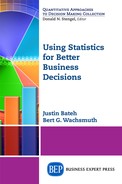
The other data column has the box plot shown in Figure 3.7 (it has two outliers on the right). The distribution is shifted to the right, and the mean should be greater than the median (the exact numbers are: mean = −0.3192, median = −0.4061).

Figure 3.6 Box plot skewed to the left

Figure 3.7 Box plot skewed to the right

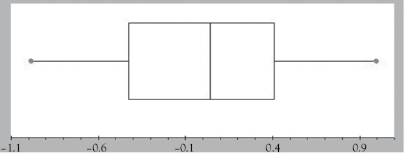
Figure 3.8 Box plot for normal distribution

The final data column has the box plot shown in Figure 3.8. The distribution is (approximately) normal, and the mean and median should be similar (the exact numbers are: mean = 0.013 median = 0.041).

Unfortunately, we forgot to write down which of these cases correspond to varA, varB, and varC—can you figure it out?

Outliers and the Standard Deviation

We have seen that even though the box plot does not explicitly include the mean, it is possible to get an approximate idea about it by comparing it against the median and the skewness of the box plot:

• If the distribution is skewed to the left, the mean is less than the median.
• If the distribution is skewed to the right, the mean is bigger than the median.

In a somewhat similar fashion you can estimate the standard deviation based on the box plot.

Another useful application for the IQR is to define outliers.

The data ranges from 0 to 491 (from minimum to maximum), while Q1 = 86.5 and Q3 = 251. Thus, we have two estimates for the standard deviation:

• s is approximately equal to range/4 = 491/4 = 122.75.
• s is approximately equal to 3/4 * IQR = 0.75 * (251 − 86.5) = 123.375.

The estimates are pretty close to each other and since the true standard deviation is 119.5, they are both pretty close to the actual value. The best part of these estimates is, however, that they are very simple to compute and thus they give you a quick ballpark estimate for the standard deviation. As for any outliers, they would be data values:

• Above Q3 + 1.5 * IQR = 251 + 1.5 * 164.5 = 497.75: none
• Below Q1 − 1.5 * IQR = 86.5 − 1.5 * 164.5 = −160.1: none

So there are no outliers in this case (which is one reason why the estimate of range/4 works so well).

For that data set we found that IQR = 78.3 − 66.85 = 11.45 and therefore the outliers would be data values:

• Above Q3 + 1.5 * IQR = 78.3 + 1.5 * 11.45 = 95.475
• Below Q1 − 1.5 * IQR = 66.85 − 1.5 * 11.45 = 49.675

Thus, two data points for South Africa (49.56) and Chad (49.44) are outliers below, while there are no outliers above. Note that since there are outliers, the range/4 estimate for the standard deviation should not work as well as the estimate based on the IQR. Confirm that!

Descriptive Statistics Using Excel

Excel of course provides simple functions for computing measures of central tendency:

Let us use our new formulas on an interesting data set: the salaries of Major League Baseball (MLB) players from 1988 to 2011.

Figure 3.9 shows the formulas that were used together with the resulting values. The mean is $1,916,817, which is indeed very different from the median of $565,000. To explain the difference, we also computed the skewness factor, which is 3.0. That means that the distribution is (heavily) skewed to the right, that is, there are a few exceptionally large values that will pull the mean up above the median. Indeed, there are a few superstar baseball players who impact the mean but not the median. Leading the pack is Alex Rodriguez from the New York Yankees with $33,000,000 per year in 2009 and 2010 and a combined salary of over $284,000,000 between 2001 and 2011. Most players do not come close to this figure; in fact, 50 percent of players make less than the relatively modest $565,000, since that is the median.

For the fun of it, we used the pivot tool to compute the average salary per ball club for the combined years (see Figure 3.10). As most of you probably suspected, the team with the highest average salary (by far) is the New York Yankees, followed by the Boston Red Sox and the New York Mets. Bringing up the rear are the Washington Nationals and the Pittsburgh Pirates.

Figure 3.9 Mean, mode, and median for MLB data

Figure 3.10 Average salaries per ball club in MLB

In addition to measures of central tendency, Excel also provides formulas to compute range, variance, and standard deviation:

=max(RANGE) − min(RANGE)	Computes the range as the maximum minus the minimum value.
=var(RANGE)	Computes the variance (ignores cells containing no numerical data).
=var.p(RANGE)	New function to compute the population variance.
=var.s(RANGE)	New function to compute the sample variance.
=stdev(RANGE)	Computes the standard deviation (ignores cells containing no numerical data).
=stdev.p(RANGE)	New function to compute the population standard deviation.
=stdev.s(RANGE)	New function to compute the sample standard deviation.

All that is involved here is adding the appropriate formulas to the Excel worksheet (see Figure 3.11).

Note: The variance is displayed as dollars, even though that is not correct (it should be “square dollars,” which does not make much sense). The standard deviation, on the other hand, has indeed dollars as unit.

There are a number of additional statistical functions that can be used as needed but Excel also provides a convenient tool to compute many of the most commonly used descriptive statistics such as mean, mode, median, variance, standard deviation, and more all at once and for multiple variables simultaneously.

Figure 3.11 Mean, range, variance, and standard deviation of salaries

Load the data set as usual. Then switch to the Data ribbon and pick the Data Analysis tool from our ToolPak on the far right. Select the Descriptive Statistics tool. Define as range the second and third columns titled “Life Expectancy” and “Literacy Rate” from B1 to C206, check the box “Label in First Row,” and check the option “Summary Statistics.” Then click OK.

Excel will compute a variety of descriptive statistics all at once and for all (numerical) variables in the selected range; Figure 3.12 shows the output.

We can see, for example, that for the average “Life Expectancy” we have computed the mean to be 71.68, the median to be 74.2, and the mode to be 76.4. The standard deviation is 8.77, the variance is 76.96, and the range is 40.2. Both variables have a distribution that is skewed to the left and hence the mean will be smaller than the median. Note that variance and standard deviation refer to the sample variance and standard deviation formulas.

Figure 3.12 Output of Excel’s descriptive statistics procedure

Using Excel to Find Percentiles

Of course Excel can be used to find percentiles, and therefore upper and lower quartiles (which are just the 25th and 75th percentiles, respectively):

=quartile (RANGE, N)	Computes the lower quartile if N = 1, the median if N = 2, or the upper quartile if N = 3. Note that Excel uses a slightly different method to compute the quartiles from that described in the “Quartiles and Percentiles” section.
=percentile (RANGE, P)	Computes percentiles, where RANGE is a range of cells and P is the percentile to compute as a decimal number between 0 and 1. The data does not have to be sorted.
=percentrank (RANGE, X)	Computes the rank of a value x in a RANGE as a percentage of the data set (in other words, the percentile value of x). The data does not have to be sorted.

Note: the QUARTILE function used in Excel uses a definition that is slightly different from our (second) one earlier. Thus, you cannot use Excel to check your own manual answers in many cases. In fact, the calculation of the quartiles is different depending on the text or computer/calculator package being used (such as SAS, JMP, MINITAB, Excel, and TI-83 Plus); it turns out that Excel alone offers two functions to compute quartiles: QUARTILE.EXC and QUARTILE.INC (which is the same as our familiar QUARTILE function). Check the article at www.amstat.org/publications/jse/v14n3/langford.html for more details.

We can use either the percentile or the quartile function to find the percentiles, or manually compute them. For the variable “Life Expectancy”:

• =percentile(B2:B206, 0.25) or =quartile
  (B2:B206,1) gives 67.1 as Q1
• =percentile(B2:B206, 0.75) or =quartile
  (B2:B206,3) gives 78.0 as Q3
• =0.25 * N = 51.25, so we pick the number at position 52, which is 67.1
• =0.75 * N = 153.75, so we pick the number at position 154, which is 78.0

For the variable “People who Read”:

• =percentile(C2:C206, 0.25) or =quartile
  (B2:B206,1) gives 81.4 as Q1
• =percentile(C2:C206, 0.75) or =quartile
  (B2:B206,1) gives 98.9 as Q3

To find the relative ranking (aka percentiles) for Japan, the United States, and Afghanistan we use the “percentrank(range, x)” function where we substitute the life expectancy of the respective countries for x:

• =percentrank(B2:B206, 50.5) = 0.014. Afghanistan is at the 1.4th percentile in life expectancy, that is, about 1.4 percent of countries have shorter and 98.6 percent have longer life expectancy than Afghanistan.
• =percentrank(B2:B206, 84.5) = 0.99. Japan is at the 99th percentile in life expectancy, that is, about 99 percent of countries have shorter and 1 percent has longer life expectancy than Japan.
• =percentrank(B2:B206, 79.6) = 0.828. The United States is at the 82.8th percentile in life expectancy, that is, about 82.8 percent of countries have shorter and 17.2 percent have longer life expectancy than the United States.

Drawing a Box Plot With Excel

Unfortunately Excel does not have a nice built-in facility to quickly create a box plot. You could of course use the formulas introduced earlier to compute the values needed and then draw a box plot manually. However, there is an easy-to-use Excel template that is not quite as convenient as the data analysis tools we have been using, but it is still pretty simple and useful. To use the Excel box plot template, click on the following icon to download the file:

When you open the file, Excel will show you a worksheet with a finished box plot already, and a column on the right in green where you can enter or paste your data (see Figure 3.13).

Figure 3.13 A box plot generated by an Excel template

Figure 3.14 Box plot generated by Excel template for life expectancy data

Simply delete the data currently in column M and replace it with your new data to create a new plot. The box plot will update automatically.

When the spreadsheet opens up, mark all numerical data in column B (the life expectancy column) but not including the column header and copy it to the clipboard (e.g., press CTRL-c). Then open the boxplot.xls spreadsheet and position your cursor to the first data value in column M. Paste the copied data values (e.g., press CTRL-v) into that column and the box plot will automatically update itself as shown in Figure 3.14.

If your picture looks slightly different, you can double-click the horizontal axis to adjust the scale (minimum and maximum) so that the picture looks like that in Figure 3.14. We can see one outlier value on the left (check if there really are extreme values according to our definition) and it seems that the distribution is skewed to the left. Thus, we would expect the mean to be less than the median (verify that).

Excel Demonstration

Company S would like to better describe the processing times of tax returns for small businesses to future clients. To do so, Company S collected the processing time in days for the last 27 tax returns (see Table 3.10). What would we tell a potential client about the expected processing times for tax returns?

Figure 3.15 The analysis ToolPak functions available

Step 1: Enter the data in two columns, labeled “Return ID” and “Processing Time” into Excel.

Step 2: Let us describe the data by finding out the mean, median, first quartile, third quartile, range, interquartile range, and standard deviation. We can find many of these using the Analysis ToolPak “descriptive statistics” function, or we can use Excel formulas. In the Analysis ToolPak, click on Descriptive Statistics as shown in Figure 3.15.

Then, for the input range select the data, check Labels in first row since we included the labels, and click Summary statistics as shown in Figure 3.16; then click OK.

We are provided with the descriptive statistics for processing time and return ID. Note we will not need data for Return ID for our analysis. Figure 3.17 shows the output of the procedure.

From this table we can now see the average processing time, median processing time, range, and standard deviation. We can find the remaining required statistics using the formulas shown in Figure 3.18.

Figure 3.16 Available parameters for descriptive statistics procedure

Figure 3.17 Output of the descriptive statistics procedure

Figure 3.18 Computing various statistics using individual Excel commands

In conclusion, we can tell our potential client that the average processing time is around 44 days, and that based on the positively right skewed statistic, we expect most of the processing times to fall toward the lower portion of the distribution, so that there is hope that the actual processing time might be shorter.