3

AFTERGLOWS

We can cheer ourselves up by recalling that it is more elevated to make predictions than to explain phenomena a posteriori.

—Sir Martin J. Rees,
Royal Astronomical Society Presidential Address
11 February 1994

 

 

Had Ray Klebesadel and his collaborators found convincing evidence for a connection of a GRB to a supernova, the search for late-time emission after a given GRB would have been sharpened and honed from the outset. Instead, the search for afterglows was generally fragmented, unfocused, and, for decades, unmotivated by specific theoretical predictions. In the context of Galactic models of GRBs, the possibility of delayed emission at X-ray wavebands was quickly hypothesized.¹ But until BeppoSAX, there was no X-ray facility that could quickly be trained on new GRB positions to search for afterglows; likewise, no convincing signatures would be seen in archival X-ray survey data.² While no obvious optical or radio counterpart was known, it was natural to expect—as an extrapolation of the spectrum of the prompt gamma-ray and X-ray emission itself to lower energies—detectable short-lived emission at longer wavelengths.³ We will refer to such light as emission of a “prompt counterpart.”

Though in the early 1990s the cosmological fireball model was far from established observationally, theorists began to wonder, in the context of this model, what would happen to that residual energy in the outward flow that was not carried away during the GRB. Bohdan Paczyski and James E. Rhoads at Princeton University, making an analogy to supernovae and the bright radiating remnants of ancient supernovae, suggested that the blastwave would slow down as it interacted with the surrounding gas and dust and eventually become large enough for radio light to escape.⁴ Concerted searches for radio afterglows in IPN error boxes gained steam but proved unsuccessful.⁵ By 1996, Peter Mészáros (Pennsylvania State University) and Martin J. Rees (Cambridge University) began developing a detailed theory of afterglows,⁶ positing that long-lived emission should be observed at all wavelengths—a panchromatic phenomenon—as a natural consequence of synchrotron emission from a decelerating blastwave. Though no convincing afterglow had been found to date,⁷ the afterglow revolution beginning the following year would quickly confirm the basic theory. In what follows, we present the panchromatic observations of GRB afterglows, and then, in §3.2, we discuss afterglow theory and its significant modifications over the years.

3.1 Phenomenology

The moment when the prompt counterpart emission ends and when the afterglow phase begins is largely subjective. It is convenient to establish the end of the prompt phase as when the gamma-ray activity appears to have ceased. This demarcation, however, builds in an obvious set of detector- and distance-dependent biases. Instead, letting theory explicitly inform our understanding of observations (often a very good idea!), we might assign the afterglow label to any emission that we believe does not come from the same physical processes that produce the GRB itself. With this notional definition, we now review the temporal and spectral properties of afterglows as seen across the electromagnetic spectrum.

3.1.1 High-Energy Afterglows

The first GRB afterglow was discovered at X-ray wavebands following GRB 970228 by the BeppoSAX team. A fleeting pulse of X-ray light during the event⁸ was caught with the WFC allowing a good initial position (~3 arcminutes radius) to be extracted from ground-based analysis. Eight hours later, using more sensitive instruments, an X-ray source ~10,000 times fainter than the initial X-ray event was seen. A few days later this source had faded by more than a factor of twenty, confirming both the spatial and temporal coincidence with the GRB; Nature would have had to be unfathomably pernicious to throw at us an unrelated yet remarkable X-ray event at nearly the same time and place as a GRB. X-ray afterglows, this first being a prime exemplar, remain the primary gateway to precise (arcsecond) localizations of all new GRBs. And so the discovery of the long-lived X-ray afterglow of GRB 970228 not only opened up a new observational channel to study the physics of GRBs but also set the stage (for the next decade and beyond) of how GRBs would be followed up at all wavebands.

For the first few years following GRB 970228, X-ray afterglows were observed in the hours to days after dozens of GRBs,⁹ mostly by BeppoSAX but also, on occasion, with the U.S. satellite Chandra, the European satellite XMM-Newton, and the Japanese satellite ASCA. The data were generally consistent with a powerlaw decay in time and with a powerlaw spectrum.^* If we parametrize the flux in time since the trigger (t) and observed frequency (ν)as

then most of the X-ray afterglows observed beyond ~1 day (≈10⁵ sec) were consistent with α ≈ −0.8 to −1.2 and β ≈ −1 to −2.

Though the X-ray data were sparsely sampled, especially after the first few hundreds of seconds and before the first several hours, some exceptions to the powerlaw rule emerged. GRB 970508 showed some evidence for a ~ day-long brightening above a powerlaw extrapolation, starting about one day after the trigger. GRB 011121 and GRB 011211 both showed bright flares at X-ray wavebands hundreds of seconds after the main activity in the gamma rays had ceased; these events also showed marginal evidence for a steepening (“break”) of the X-ray powerlaw decay at later times (well after one day).¹⁰

Swift, by not requiring laborious ground-based analysis to search for precise X-ray positions, can train the XRT at new GRB positions in less than a minute and can continue to return to that position for as long as the afterglow remains visible. More than 95 percent of Swift GRBs have led to the detection of X-ray afterglows. As such, Swift opened up a more complete view of X-ray light curves, starting seconds after the trigger and lasting for days. The upshot was a rather startling discovery: deviations from a simple X-ray powerlaw decline are themselves the rule not the exception.¹¹ Indeed, only in a few cases (e.g., GRB 061007) out of hundreds is a pure powerlaw decline at X-ray wavebands observed. Instead a rather complex picture of the afterglow has arisen. Figure 3.1 shows a schematic of what is now the “canonical” X-ray light curve, exhibiting a number of distinct phases. Though there is of course a wide range of observed behavior, in general the earliest X-rays appear to be a lower-energy extension of the prompt gamma-ray emission. This is then followed by a steep decline, where the X-ray light dims by several orders of magnitude in just a few hundreds of seconds (here the α decay constant is −3). After the steep decline, a shallow-plateau (α ≈ −0.5 to 0) phase begins, lasting for tens of thousands of seconds. Then, typically a few hours after the trigger, a more rapid decline sets in (α ≈ −1.2), which sometimes leads to a more rapid decline (α ≈ −2) at late times.^* Until Swift, only the first and last (two) phases were routinely observed, which might help explain the apparent powerlaw simplicity of the late-time pre-Swift X-ray afterglow population.

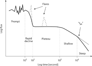
Figure 3.1. Canonical X-ray light curve following the evolution from the time of the GRB trigger. The prompt phase generally tracks the light curve behavior of the gamma rays. A short-lived period of rapid decline is then often seen, where the afterglow plummets in flux over a short period of time. A period of relatively steady flux follows, called the “plateau” phase. The “shallow” and the “steep” phases are seen after several hours. The transition (“break”) from shallow to steep is often referred to as the jet break time (t_jet). Bright pulses seen after the prompt phase are called “flares.” There are many variations on this general picture; some real light curves are shown in figure 3.2. Adapted from B. Zhang, Y. Z. Fan, J. Dyks, S. Kobayashi, P. Mészáros, D. N. Burrows, J. A. Nousek, and N. Gehrels,ApJ 642, 354 (2006).

Flares: Rapidly rising and falling behavior is, of course, the hallmark of what we call the prompt emission. X-ray flares/pulses during this early time are simply attributed to the same emission processes that create the gamma rays. In many cases, X-ray flaring ceases before the onset of the rapid-decline stage (at a few hundred seconds). However, many events show up to a few X-ray pulses during the rapid decline and plateau phases. The energy contained in such pulses is generally a few percent of the total energy in the prompt emission (though in extreme cases the energy can be comparable). In most X-ray flares after the prompt emission, the total duration of the flare appears to be about 10 percent of the time since the trigger—that is, the longer it has been since the trigger, the longer an X-ray flare lasts. There are some counterexamples to this rule of thumb, however: Chandra X-ray observations following the short-duration GRB 050709 showed a flare more than one day after the GRB, but this flare lasted less than a few hours.¹² We will discuss the interpretations and importance of flares in §3.2.1.2 and §5.2.3.

3.1.1.1 Spectral Features

The analog to temporal breaks are departures from powerlaws in the spectral domain. Spectral features can be either in the form of absorption (less flux than we expect) or emission (more flux).

Absorption: Several GRB X-ray afterglows appear to show evidence for a rollover at low energies (see figure 3.3). This apparent absorption—which of course requires us to assume what the afterglow would have looked like without absorption—is usually attributed to suppression (commonly referred to as “attenuation”) of the emergent afterglow light by the material in between us and the GRB. It manifests itself as an energy-dependent optical depth (with τ E^−8/3) and is attributed to interaction of X-ray photons with common atoms in the Universe (H, He, C, O, and so on). The degree of this interaction is measured as the “photoelectric cross-section” because when a photon of a certain energy or higher interacts with an electron in one of these atoms on its otherwise merry way to our detector, there is some chance it will instead get absorbed by that atom. Its deposited energy is then used to liberate a bound electron, causing that atom to be ionized. The normalization of the optical depth is then just proportional to the amount of absorbing atoms along the line of sight.^* We can use the observed amount of absorption to infer something about the average properties of the gas and dust in the regions around the GRB and in the galaxy where it occurred.^† Interestingly, the inferred amount of absorption in the host galaxies of GRBs is larger, for most events, than the degree of absorption we would expect to find if we poked random sightlines through the Milky Way. The implication of this will be discussed further in §6.2. It is also worth noting that there have been controversial claims of a changing (both increasing and decreasing) amount of apparent absorption in a few GRB X-ray afterglows. Increasing absorption is very difficult to explain physically but could be explained away by invoking intrinsic curvature of the afterglow spectrum (as might be expected from a Band-like spectrum [§2.1.1], instead of the usually assumed intrinsic powerlaw).

Emission: In the first few seconds of a GRB, more than 10⁵⁵ high-energy photons start streaming out from the source. If there is any material around the GRB—in the circumburst environment—it will certainly notice the deluge of these photons. Lighter elements, like hydrogen and helium, will almost certainly be completely ionized but heavier elements, like iron (Fe) and nitrogen (N), may retain some of their electrons. Some of the electrons may be pushed to an excited state by the high-energy photons but rapidly fall back to lower-energy states and, in doing so, emit lower-energy photons at specific wavelengths. This process is called “fluorescence” and is the same physical process that makes the emitted spectrum of fluorescent lights and the beautiful colors in Hubble Space Telescope images of planetary nebulae. In the BeppoSAX era there were claims of X-ray line emission in some GRB afterglows, which were interpreted as being due to large amounts of iron around the GRB, a potentially very important clue to the progenitors. Unfortunately, the evidence for line emission was never very strong, and after a few years of controversy about the statistical significance of line claims¹³ coupled with the lack of significant line detections in Swift GRBs, the existence of X-ray line emission in GRB afterglows does not appear to have stood the test of time.

3.1.1.2 Gamma-Ray Afterglows?

There is, of course, nothing special about photons observed with energies within the arbitrarily defined X-ray bandpass. So the natural expectation is that afterglows should be manifest at higher and lower energies. Prompt variable emission of the GRB itself very often outshines the expected gamma-ray afterglow light, but there is good evidence from BATSE that many long-duration GRBs show evidence for low levels of smoothly decaying gamma-ray light following each event.¹⁴ Some of the brightest events, particularly GRB 980923 and GRB 920723, show not only clear evidence for a long-lived smooth component of gamma-ray emission after the main variability has ceased but that this emission is dramatically softer than the spectrum of the prompt GRB.¹⁵ Interestingly, long-lived emission detected by Fermi at the very highest energies (> 100 MeV) appears to be well accommodated¹⁶ by a simple theory for the afterglows (see §3.2.1). That is, afterglows appear to be pervasive phenomena from GeV to keV energies.

3.1.2 Ultraviolet-Optical-Infrared Afterglows

The discovery of an X-ray afterglow in GRB 970228 was followed by the discovery of an optical afterglow coincident with the initial ~3 arcminute WFC localization of the prompt emission and the X-ray afterglow itself. X-ray-afterglow discovery has become an important part of what is now a routine chain of observations: crude prompt gamma-ray localizations lead to X-ray-afterglow discoveries which lead to optical afterglow discovery.¹⁷ However, the discovery rate of optical afterglows is not nearly as high as with X-ray afterglows: only about 50 percent of Swift GRBs have a detected afterglow at optical, infrared (IR), and/or ultraviolet (UVOIR^*) wavelengths (although the majority of the nondetections can be understood as due to insufficiently sensitive searches). In §6.2 we will discuss the nature and importance of “dark bursts,” a label ascribed to the ≈10–15 percent of events where no good optical afterglow was found despite exhaustive searches.¹⁸

At very early times, while the gamma-ray activities are in progress and just after, the UVOIR behavior is less well studied. Less than two dozen GRBs have contemporaneous measurements of long-wavelength and gamma-ray emission. For logistical reasons^† such events tend to be the longer-duration GRBs, and, clearly, the brighter the afterglow the better the chance that small and nimble telescopes have for detecting the afterglow. The first contemporaneously detected optical afterglow was GRB 990123, found with the Robotic Optical Transient Search Experiment (ROTSE). The extreme peak brightness of that afterglow (magnitude 9 in the visual band) was far exceeded by the fifth magnitude^* afterglow of GRB 080319b.¹⁹ The first contemporaneous near-infrared afterglow was found by my group²⁰ at Harvard University and UC Berkeley following an Integral/Swift event (GRB 041219b). To date, no contemporaneous UVOIR observations have been made for a short-duration GRB, most likely because the afterglows of such events are intrinsically fainter than for long-duration GRBs.

Those events with early UVOIR light curves show a wide diversity of behavior (see figure 3.2), from monotonically declining to long-lived plateaus to fastand slow-rising “morphology.”²¹ When correcting for the cosmological time-dilation effect, all afterglows appear to be fading after about ten minutes in the comoving frame, and the intrinsically brighter the afterglow is after 400 seconds, the faster it appears to fade.²² There have been a few suggestions that some contemporaneous optical light curves move in lock step with the prompt gamma-ray-emission light curve. However, most UVOIR light curves are not correlated with the GRB, appearing instead to follow the beat of their own drum. This suggests that the UVOIR afterglows are likely due to a different emission mechanism and/or emission site than the high-energy prompt emission.

Those GRBs with detected UVOIR afterglows provide a direct probe of the physics of the emission at late times from the events. Just as with X-ray afterglows, the nominal theoretical expectation—that of a powerlaw spectrum decaying like a powerlaw in time—appears to be crudely borne out. However, just as with X-ray afterglows, there are important departures. Many of the best-studied afterglows show small-scale (< 10%) variations about a powerlaw decline for hours to days after the trigger. Some show evidence for flaring more than thousands of seconds after the prompt emission has ceased.

Figure 3.2. Some gamma-ray, X-ray, and optical light curves with good early optical coverage. Some of the light curve features discussed in the text are shown, such as plateaus, flares, and powerlaw declines. Adapted from E. S. Rykoff et al.,ApJ 702, 489 (2009).

There are significant departures in the spectrum of UVOIR afterglows from the nominal powerlaw expectations. There are smooth absorption features across these bands that are attributed to obscuration by dust. Dust pervades the universe (not just your living room) and is thought to be carbon- and silicon-based molecules ranging in size from a few microns to a few millimeters.²³ We believe that dust forms in the ejected material of some supernovae explosions as well as the sloughed-off envelopes of dying stars. Since it is this same “star stuff” that comprises the building blocks of stellar nurseries and stars, it is not so surprising at all that we should see its effects in very distant galaxies. Afterglow light passes through dust where its red light preferentially penetrates through the material and its blue light preferentially scatters; this is essentially the same physical interaction in the atmosphere that causes blue skies and red sunsets on Earth. So a generic property of dust is a systematic suppression of the bluest light. Figure 3.3 shows some examples of the effects of dust on afterglows. Aside from the broad dust-induced curvature, there is also a rich diversity of much more narrow absorption features in UVOIR afterglows that are due to molecules and atoms blocking certain frequencies of afterglow light. These narrow absorption lines are both telltale tracers of the redshift of a given GRB and useful in probing both the environment around the GRB and the pollution history of heavy elements throughout the Universe (chapter 4 and §6.1).

After accounting for these various roots of absorption, the intrinsic late-time spectra and light curves of UVOIR afterglows are reasonably characterized as powerlaws declining in time and frequency (see equation 3.1). Typical values²⁴ for the powerlaws are β ≈ − 0.7 ± 0.2 and α ≈ − 1.1 ± 0.3. If we were to integrate this f (ν, t)from zero to infinity in time and in frequency, we would be faced with the uncomfortable inference of infinite energy release, and so it is clear that this formulation must only be relevant in a restricted range. We have already seen that for the earliest optical afterglow observations, the light curves are seen to rise (taking care of the integration problem at early times). At late times, so long as f (t) where the critical index α_c < −1, then we also have a finite contribution to the energy release. The implication is, of course, that if α ≥ −1 during some point of the afterglow phase, the light curve must eventually bend downward. Indeed, many “breaks” are seen in GRB afterglows and we will discuss them in §3.3.

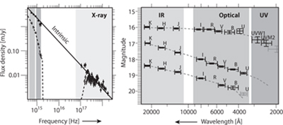
Figure 3.3. Extrinsic absorption of GRB afterglows at UVOIR and X-ray wavebands. (left) Modeled photoelectric absorption at X-ray wavebands and dust extinction at optical and UV take the observed data (lower points) to unextinguished data (higher points), showing consistency with an intrinsic smooth powerlaw spectrum (solid curve) from optical to X-ray. This GRB (070318) is thought to have one of the largest dust- and photoelectric-absorbing columns seen in GRBs. Note how the UV light (middle gray vertical region) is much more suppressed from the intrinsic powerlaw spectrum relative to the low-frequency data. Adapted from P. Schady et al., MNRAS,401, 2773 (2010). (right) Three UVOIR afterglows showing little-to-moderate amount of dust extinction. The filter names above each data point are shown. Adapted from a figure provided by D. Perley.

3.1.3 Long Wavelengths

At wavelengths longward of UVOIR bands lie the far-infrared, sub-millimeter, millimeter, and radio wavebands. Afterglow coverage and detection in this regime are significantly more sparse and infrequent than at UVOIR bands. However, the events that are detected at long wavelengths tend to provide some of the greatest insight into the nature of the afterglow and the burst itself. GRB 970508 was, of course, a watershed event that settled the great debate over the distance scale of GRBs (§1.6), but it also marked the first detection of radio and millimeter afterglows. The first sub-millimeter detection was with GRB 980329. Of the pre-Swift GRBs there were twenty-five radio afterglow detections (about one-third of the total localized GRBs), and a roughly comparable number were found in the first five years of the Swift era (thirty-two afterglows until January 2010). The vastly lower detection rate is attributed to the higher median redshift of Swift events and the fact that even the best radio and millimeter receivers are relatively less sensitive to afterglows than optical instruments.²⁵

Unlike UVOIR afterglows that reach peak brightnesses within minutes of the GRB trigger, most radio afterglows peak only after days to weeks (see figure 3.4). There is a small minority of radio afterglows that appear to peak within a few days of the GRB trigger, then decline rapidly, only to rise again on days-to-weeks timescales.

Figure 3.4. Four of some of the most extensively covered radio-afterglow light curves of GRBs discovered before the Swift era. The observed fluxes are shown along with the measurement uncertainties (vertical lines at each data point) in the fluxes; arrows represent nondetections. The solid lines show the model fits to the data (including extensive data at other wavebands not shown here; see §3.2). The gray areas represent the expected envelope of characteristic flux variability due to “interstellar scintillation.” All these events took more than one week to reach maximum flux in the observed waveband of ν = 8.4 GHz. The flattening of the light curves at late times may be due to the transition of the blastwave from being a relativistically expanding source to a nonrelativistic source but may also be due to a contribution from a radio-bright host galaxy; see D. A. Frail, B. D. Metzger, E. Berger, S. R. Kulkarni, and S. A. Yost,ApJ 600, 828 (2004). Adapted from S. A. Yost, F. A. Harrison, R. Sari, and D. A. Frail,ApJ 597, 459 (2003).

The best-studied radio afterglows appear to have erratic flickering behaviors at some observed wavebands. This flickering, first seen in GRB 970508, is attributed to so-called “interstellar scintillation” (ISS), a phenomenon also seen with other radio sources (like quasars and pulsars).²⁶ The key ingredients to ISS are a radio source with an inherently small size and the propagation of the radio light through a clumpy medium full of free (i.e., unbound) electrons. The electrons act as a refractory material that bends radio light, serving to amplify and dim the total intensity in different directions. Think of the bright and dark pattern on the bottom of a swimming pool on a sunny day: as you move along the bottom of the pool, just as the Earth moves through the radio-amplification pattern, you would see the light source get brighter and fainter with time. Depending on the wavelength of light, the amount and location of the “screen” of electrons in the Milky Way, and the relative distances from the Earth and the radio source to the screen, the degree of changing of amplification can be predicted from our knowledge of the electron distribution in the Galaxy provided we know the apparent size of the radio source. The bigger the radio source, the less scintillation we expect; essentially, the larger the apparent size of the source, the more the twinkling or scintillation effects are washed out. This is very similar to the reason planets in the Solar System do not appear to twinkle at night whereas stars at the same elevation above the horizon do.

What is so remarkable about ISS as a tool is that it allows us to make an inference of the size of the radio source even if we cannot directly resolve the source image with our equipment. In the case of GRBs, as seen in figure 3.4, it is the gradual suppression of scintillation that tells us not only that the radio source is getting bigger with time but also how physically big it would be if we could measure it directly. Thus, the consequence of the radio light curve of GRB 970508 coupled with the extragalactic distance measurement was to confirm one of the basic suppositions of GRB theory: the afterglow light was produced with a source expanding at a velocity near that of the speed of light.²⁷ This remarkable conclusion is reached with very little appeal to the nature and physical origin of the radio source itself. Six years later, the radio afterglow of GRB 030329 was observed at high image resolution, allowing a direct measurement of the expansion rate of the blastwave: more than one month after the event, the blastwave was inferred to be expanding relativistically with Γ ≈ 7. These observations²⁸ of GRB 030329 remain the simplest and most robust evidence to date for the relativistic nature of GRB outflows.

3.2 Origin of the Emission

The Mészáros and Rees theory of afterglows²⁹ arrived just in time to give physical context to the discovery of the first afterglows. At its heart, the theory posits that the same blastwave that makes the prompt emission continues to expand into the ambient medium. Eventually, just as an American football linebacker plows his way through a sea of massive bodies, the blastwave loses steam and slows up as it is bombarded by what appears to be the oncoming mass of the circumburst material.

In this deceleration, the kinetic energy tied up in the outward flow gets channeled into random motions of electrons, protons, and neutrons behind the head of the blastwave. An external (collisionless) shock is formed (§2.2.2), which we call the forward shock. For essentially the same physical reasons that the internal shock releases gamma-ray light (§2.3.3), this “hot” blastwave now begins to radiate (albeit at longer wavelengths than during the prompt phase). The dominant emission mechanism of afterglows is thought to be synchrotron radiation (radiating relativistic electrons in a magnetic field), just as is the apparent origin of the prompt emission. Since the characteristic energies of the relativistic electrons—which directly translate into a characteristic peak in the resultant spectrum—are connected to the bulk speed of the blastwave, the emergent spectrum and the overall evolution of the blastwave are inexorably linked.

Like all good physical theories that stand the test of time, the so-called synchrotron blastwave theory provides a very good framework for understanding observed afterglows, and (perhaps more importantly so) it has made predictions that have been borne out by observations. Indeed one of the first papers of the afterglow era by Ralph Wijers and collaborators³⁰ noted the broad agreement between the Mészáros and Rees theory and the gamma-ray, X-ray, and optical observations of GRB 970228. Yet, despite many successes, the original theory clearly fails to anticipate and explain the rich phenomenology of afterglows as observed since 1997. As such, it suffices to state here that the theory is itself an evolving one, having been both refined and added to as the data have demanded. Much of the early-time afterglow data, particularly at X-ray and UVOIR wavebands, continues to present significant challenges to the current incarnation of the theory and certainly requires extensions beyond the most simple picture. We discuss the salient features of the theory in what follows and then introduce extensions to the theory in the later sections.

3.2.1 Synchrotron Blastwaves

In the simplest treatment, we posit that the decelerating blastwave is producing afterglow light as it expands “adiabatically”—that is, we assume that the amount of energy carried away by the afterglow light is an insignificant fraction of the total blastwave energy. The attractiveness of this supposition (other than it appears to be true at late times) is that it allows us to decouple the consideration of the dynamics of the blastwave and the calculation of the emission. If the afterglow does carry away a significant fraction of the blastwave energy, then we would say that the afterglow is “radiative,” and we would necessarily have to treat simultaneously how the blastwave evolves in time and what spectrum is emitted.

3.2.1.1 Dynamics of an Adiabatic Blastwave

On simple conservation-of-momentum grounds, in “ordinary” explosive events (like those in SNe and atom-bomb detonations), we expect significant deceleration of the outward flow when the ejected material sweeps up from the ambient medium a total mass roughly equal to that of its own mass. However, in relativistic flows like in GRBs, the ambient material of mass M_ambient appears^* to the outflowing material to have an increased mass M_{apparent, ambient} = Γ M_ambient. Since the typical Lorentz factors at the time of the internal shocks is Γ ~ 100 (§2.2.1), this means that the deceleration begins when only about 1 percent the mass of the ejected material (ejecta), M_ejecta, is encountered. For a GRB with E_γ = 10⁵¹ erg release, this implies^† that the afterglow phase begins after about M_ambient = 10²⁷ gm of material is swept up. Under the simplest assumption, we take the number density of particles n around the GRB to be constant and about equal to that of the density of hydrogen in the interstellar medium of our Galaxy; that is n = 1 cm⁻³. Therefore, the mass swept up by the blastwave at radius r is just the volume times the mass per particle (m_H = 1.674 × 10⁻²⁴ gm) times the density of particles.

Setting this equal to M_ambient = E_k/ (Γ²c²)we have

Thus, for typical parameters, the deceleration begins when the source has reached about 3,500 astronomical units [AU], roughly one hundred times the size of the orbit of Pluto. Traveling at nearly the speed of light, it would take the blastwave about twenty days to reach this radius. But because of time compression for distant observers, we see this deceleration occur much more quickly by a factor of ~2 Γ²; for us, the blastwave appreciably decelerates in just a few minutes or less.³¹ Indeed if we associate the brightest moment in the early afterglow with this deceleration time, we could use the afterglow peak time to estimate the initial Lorentz factor.³²

It is clear from equation 3.2 that if the total energy in the blastwave remains roughly unchanged in the adiabatic phase (E_k ≈ constant), then the Lorentz factor must decrease with increasing radius: Γ r^−3/2. Since the observer time is t_obs = r/2Γ²c (see footnote on page62), this implies that the radius of the blastwave apparently changes as r(t_obs) and that the Lorentz factor changes as Γ(t_obs) = t^−3/8. If the deceleration from Γ = 100 starts at thirty seconds, under this consideration the source becomes nonrelativistic (Γ ≈ 1) after about t_obs(nonrel) = 30 sec × 100^8/3 ≈ 2.5 months.

Of course, GRBs being more complicated beasts than perhaps we would like them to be, there are some expected modifications to this simple set of derivations. The adiabatic assumption is probably a good one at late times but we certainly do expect that the afterglow carries away a nonnegligible faction of E _k during the bright early phases. This brief radiative regime causes Γ to decrease more rapidly with radius and in time relative to the adiabatic case. Likewise, it is probably too simplistic to hold that the blastwave should be plowing into a perfectly homogeneous medium on scales of AU to parsecs. Instead, if the density around the GRB event decreases with increasing distance from the explosion site (the next simplest assumption; §4.1.1), less and less mass is swept up as the blastwave expands relative to the homogeneous case. Therefore, the blastwave will decelerate more slowly with increasing radius relative to the homogeneous case. So in rederiving the relationship between Γ and r we would need to replace nm_H in equation 3.2 with a functional form for the mass density as a function of radius. Figure 2.5 in the preceding chapter shows the dynamics of the blastwave during the (external shock) afterglow phase. The evolution of labeled “wind” (see also §4.1) assumes that the circumburst density falls as the square of the radius from the explosion site.

3.2.1.2 Spectra from the Blastwave

We now have a reasonable prescription for the radius of the blastwave as a function of time, the Lorentz factor, and the total energy. A shock will have developed at the head of the blastwave such that the properties of matter and magnetic fields will be substantially different inside and outside the shock. To calculate the emergent spectrum, we need to know the conditions within the shock. Such conditions can be derived by assuming conservation of momentum, energy, and mass. It is beyond the scope of our treatment to carry through such calculations, but suffice it to say that the density of particles is higher in the shock as is the subsequent energy per particle. Most important is the notion that these shock properties are directly related to the bulk Lorentz factor of the blastwave at a given time. So as the Lorentz factor decreases, for instance, the density of particles behind the shock also decreases. Similarly, the average energy per particle also decreases with decreasing Lorentz factor. Both of these quantities are critical for determining the emergent spectrum.

Unfortunately, basic conservation laws do not tell us uniquely what the distribution of energies are for shocked particles, nor do we have an easy route to determine the magnetic field strengths in such shocks. Like all seasoned physicists we parameterize our ignorance, taking the distribution of shocked electrons to be a truncated powerlaw^* and the magnetic-field strength to be a constant fraction of the instantaneous energy density in the shock. With these ingredients in hand, the emergent synchrotron spectrum can be calculated.

Instantaneous Snapshot: Figure 3.5 shows some snapshot spectra of GRB afterglows from radio to X-ray, comparing data and theory. The peak luminosity of the emergent spectrum is thought to come from radiation by the largest number of electrons: for the assumed electron distribution (equation 3.3), those that have the lowest energies (E_min) are the most numerous. In carrying through the calculation for peak luminosity, in the simple case of a circumburst medium that is uniform (i.e., with n = constant), the dependencies on Γ of the shock cancel out, and we are left with a constant brightness for most of the relevant observing time. The frequency at which the emergent spectrum is brightest is called the “peak” (or “maximum”) frequency, symbolized as ν_m. At frequencies higher than ν_m, the spectrum at a given time is influenced by the electrons at all energies. This portion of the spectrum is calculated to be a powerlaw f (ν) ν^β where β = − (p − 1) /2. That is, all that matters is what the slope of the electron energy distribution happens to be. At the very largest frequencies (in the UV or X-ray band initially), the slope of the spectrum is expected to be steeper. The reason for this is that the very fastest-moving electrons are actually radiating an appreciable amount of their kinetic energy quicker than electrons with those energies can be replenished by the shock. The spectral interface between the two regions is called, appropriately enough, the cooling break, and the frequency at which this occurs is denoted ν_c. At frequencies less than ν_m, the spectrum is dominated by the basic low-energy synchrotron tail of lowest energy electrons. Here β = 1/3, regardless of the value of p. At the very lowest frequencies (typically at radio wavebands), the optical depth of the blastwave is greater than one, leading to a rollover in the spectrum. The characteristic frequency ν_a of this rollover is called the “synchrotron self-absorption” frequency.

Figure 3.5. Observations and model fits to basic afterglow theory. (top) An instantaneous snapshot spectrum of the afterglow of GRB 071003 2.67 days after the GRB, showing both observed data and a synchrotron-shock model. The faint thin line that deviates from the powerlaw at UV and X-ray wavebands shows the effect of dust and photoelectric absorption (§4.1.1). The dashed line and gray wedge show the extrapolation (and uncertainty in that extrapolation) of the X-ray data to smaller frequencies. Connecting the X-ray data to the dust-corrected optical data gives an acceptable fit of β = 0.93 (see equation 3.1). The radio data are consistent with expectations of a steepening due to synchrotron self-absorption. Adapted from D. A. Perley et al., ApJ 688, 470 (2008). (bottom) Evolution of the observed spectrum in GRB 070125 with the three break frequencies labeled. Note how ν_m and ν_c appear to evolve with time. From P. Chandra et al.,ApJ 683, 924 (2008).

Evolution in Time:Since is, generally, decreasing with time, this whole snapshot spectrum should evolve in time (see figure 3.5). In the simplest case where the density of the circumburst medium is constant (see equation 3.2), the overall maximum brightness remains unchanged, but the location of this peak (ν_m) marches monotonically downward from the X-ray to the optical to the radio bands over time periods ranging from a few minutes to a few weeks. So if you were to observe at a fixed frequency—say, at optical wavelengths—you would see the source get brighter as the peak frequency starts to approach your observing band. Then, after the peak frequency moves through your band (toward smaller frequencies), you would then see the afterglow dimming. The flux before maximum appears to rise as a powerlaw and then decay as a different powerlaw. If f (t) t^α at some fixed observing band, we can calculate α under different assumptions. Importantly, after ν_m has passed through the observer’s band, α is expected to be directly related to the electron distribution index p, such that α = −3 (p − 1)/4.

The interesting ramification of this basic theory is that, if you can measure the spectral slope of the afterglow at some frequency, you can predict how the flux should change with time (and vice versa). Put another way, the evolution with time of the afterglow can be used, in principle, to infer the basic parameters of blastwave: p, Γ as a function of time, E_k, the magnetic field strength, and the density structure of the circumburst environment. Getting constraints on the macrophysical and microphysical parameters has become a small cottage industry in the GRB field. Unfortunately, however, this product line is derived from a very expensive set of raw materials: to measure uniquely and robustly the parameters of interest in a given GRB afterglow, a lot of data needs to be acquired across the electromagnetic spectrum.³³ Without good coverage, ambiguities persist about the location of the break frequencies, which lead to very different determinations of the parameters of interest.

Even in the presence of good temporal and spectral follow-up, there are several wrinkles that complicate the interpretation of the data in the context of the basic synchrotron blastwave theory:

• Light Travel-Time Effects: While the calculation of the instantaneous spectrum may be correct at a given radius and for a given Γ, the emitting region is (most simply) spherical. As a result of this and the finite travel time of light, photons emitted at the same time and radius reach the observer at different times: photons from the edge of the emitting region take longer to get to us. Put another way, at a given observer time, the observed true spectrum is a nontrivial admixture of light from material at a variety of radii and with different Γ factors. This tends to smooth out transitions across spectral breaks to the extent that an analytical calculation of the spectral breaks is inadequate to describe fully the true emergent spectra. Numerical simulations are required to produce a more realistic set of model expectations.
• Other Emission Components:

– Reverse Shocks: Under certain conditions, a “reverse” shock that moves back through the ejected mass of the blastwave may have much of its energy converted into random motions, which in turn produces a bright flare of emission that can last for minutes at optical wavebands and days in the radio. GRB 990123 and GRB 021004 are classic examples of afterglows thought to be dominated at early times by bright reverse shocks in the optical. GRB 990123 also showed evidence for a bright radio flare at early times, taken to be additional evidence of reverse shock emission.³⁴

– Inverse-Compton Scattering: If a photon produced from the synchrotron process encounters a fast-moving electron in the shock, it can be scattered to a much higher energy. Such Inverse Compton scattering (see §2.3.3) will suppress the emergent flux of low-energy photons and produce an excess of high-energy photons. Since some X-ray afterglows appear brighter than they ought to be under the simple blastwave theory, IC has been successfully invoked to explain the excess.

– Other Contributing Distributions: Even if the emergent spectrum were entirely due to synchrotron radiation by electrons, other departures from the simple spectra would occur if there was something other than a powerlaw distribution of electrons in the shock. Moreover, since we do not have a good a priori reason to expect that the magnetic field strength should be a constant fraction of the energy density in the shock, it is possible that there is a true interplay between the parameters of the shock; this would lead to differences in the evolution of the spectra. The effects of protons and neutrons in the blastwave may significantly alter the emergent spectrum.

• Other Absorption Sources: The degree of dust and photoelectric absorption in afterglows is treated as a free parameter in the comparison of data to models. But dust and atoms near the burst may be significantly affected by the afterglow light itself. So these absorption properties are expected to change with time, complicating the modeling. Atoms (including barren protons from ionized hydrogen) within the blastwave may nontrivially alter the emergent spectrum.
• Obvious Light-Curve Departures: Flares, plateaus, rebrightenings, and repeated undulations (sometimes called “bumps and wiggles”) in afterglows are not part of the basic synchrotron theory yet appear to be common among some of the best studied GRBs. Some of these effects have been modeled in the context of a long-lived central engine that replenished the blastwave with more energy well after the prompt GRB phase. Another possibility is that energy, mass, and Lorentz factors may be different in some portions of the blastwave. This is a possibility we return to in §3.3.

Some of the most active areas of research in GRBs is in understanding the relevancy of these departures from basic theory on what we observe. One of the main points of consternation is that the richness of the phenomenology of GRB afterglows has yet to be captured by a complete theoretical framework. Not only are there many free parameters in the model components that we do know about but also, when a certain afterglow cannot be fit well, new components must necessarily be envisioned. Such after-the-fact theory, even if physically motivated, tends not to be very satisfying to most scientists. It is one thing to have a set of useful model components to help give physical context to what you just saw. But, more than this, observers are especially eager for model predictions that can be falsified with new data. Perhaps the most worrying concern looking ahead is that the edifice of the synchrotron shock model has become so complex that it can only be made more complex,³⁵ but yet cannot be falsified.

Despite the many complicating components and the general concerns about complexity, some basic results appear to be robust. First, it seems as though many of the p values range from 2–2.5, nicely consistent with what is inferred in nonrelativistic supernova shocks.³⁶ Second, while the circumburst density appears to range over many orders of magnitude, with n ≈ 1 cm⁻³ (see equation 3.2) taken as the fiducial value, one of the rather interesting results is that, with only a few exceptions, the density of the circumburst medium appears to be uniform (as opposed to decreasing with increasing distance from the explosion).³⁷ Last, the efficiencies of conversion from kinetic energy to gamma-ray release appear to be about the same (η ≈ 0.01–0.1) for short and long bursts for the full range of L_k.

3.3 Evidence for Jetting

The inference of the total energy release from what we see relies on a crucial assumption about the geometry of the explosion (see figure 3.6). In the simplest case, we assume that all the energy is released isotropically (E_iso)—that is, uniformly in all directions. But our detectors, the ones that intercept those few high-energy photons from a distant GRB, cover only a tiny fraction of all the possible directions to where a GRB could emit light. Would a satellite at the edge of the Solar System with an identical detector pointed in the identical direction measure the same brightness as one near Earth? Probably. What about a satellite in another galaxy? Maybe not. At vastly different places in the Universe, there is no guarantee that the same GRB event would appear the same. Indeed, some places in the Universe would never see a specific GRB if no photons are emitted toward that specific direction. If a magnetic field axis is aligned (or nearly aligned, as in the case of the Earth) with the rotation axis, then charged particles (such as electrons and protons) naturally prefer to flow to and from this axis. All this is to say that given the preponderance of jets, especially when matter is flowing near compact objects like black holes, it is natural to posit that GRB outflow could indeed be collimated.^*

Jetting (or collimation) of mass outflows appears to be a common phenomenon. Some quasars and other “active” galaxies (with massive black holes swallowing up and spitting out matter) are seen to have narrow jets that persist all the way from parsec to Megaparsec scales. Smallmass analogs in our Galaxy, called microquasars, also show jets that contain a lot of kinetic and magnetic energy. Even newly forming star systems have jet-like outflows of mass during their creation. The physical origin of jets varies across phenomena but is not fully understood in most cases. However, when rotation is involved it is clear that the axis of rotation forms two preferred directions.

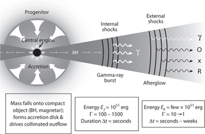
Figure 3.6. Schematic of the relevant structures, emission regions, and energetics for the internal-external shock model. The canonical energy release (using a correction for the jet opening angles) is E_γ ≈ 10⁵¹ erg. This is somewhat lower than the energy E_k entrained in the outflow. The inferred jet angles are generally smaller than shown; the typical opening angle of the jet is a few degrees. Adapted from P. Mészáros, Science 291, 79 (2001).

How could we infer the geometry of the explosion without being able to image it directly? It turns out that afterglow theory predicts a fairly robust behavior: a “break” in the light curve that happens at about the same time across the electromagnetic spectrum. A break is a noticeable downturn in a light curve; that is, before a break the flux is changing more slowly than after the break.^* The origin of this “jet break” stems both from the geometry of the explosion—in this case, some posited collimation (“jetting”) of the blastwave—and the fact that it is expanding relativistically. Basic considerations from Special Relativity show that particles moving near the speed of light appear to emit most of their energy in the direction they are heading. It is as if the faster you traveled on a dark road, the more focused your headlights would appear to become to someone watching you breeze by. Mathematically one can show that most of the energy is “relativistically Doppler beamed” into an angle of size about θ ≈ 2 / Γ (units of [radians]) when Γ is much larger than unity. So if particles in the blastwave are all moving at about Γ = 100, then anyone sitting within about one degree of the direction of motion of a given electron would see (synchrotron) light from that electron.

So as the blastwave slows down, θ increases, allowing some outside observer to see more and more of the afterglow-emitting surface. The calculation of a powerlaw decline (after ν_m has swept past the observing frequency) assumes that the observer sees more and more of a spherical explosion. What if the explosion is not spherical but more of a collimated fountain of ejecta? In this case, if you happen to be looking down the barrel of this jet coming toward you, at early times you do not notice that it is not spherical (because Γ is large and you can only see light from an angle < 2 /Γ). But later, once has Γ decreased enough, you suddenly see that there is no material at larger off-axis angles. This is the origin of the break in the light curve, and since it occurs because there are fewer-than-expected electrons radiating toward you, the break must occur at the same time across the electromagnetic spectrum. At this break time,^* the collimation angle of the jet must be comparable to 1 / Γ.

Just as α predicts β of the spectrum (see §3.1 and §3.2.1.2), so too does the value of α before the break time predict the decay rate α_post-break after the break. Indeed, in the simplest case, the flux after the jet break should drop more steeply than before as f (t) t ^{− p} (i.e., α_post-break = − p). GRB 990510 has a classic afterglow showing a break at optical wavebands (figure 3.7). This break is consistent with the break occurring simultaneously at other frequencies. Confirming a theoretical prediction,³⁸ the decay slope before the break also correctly anticipates the value of the decay slope after the break. If the collimation angle is found to be θ_j, then you can show that the true energy release in gamma rays is a factor of θ / 2 less than what you would have inferred if the energy was emitted isotropically. Since, when they are measured well, typical θ j values are in the range of a few to several degrees, this means that the true energy release in gamma rays can be 0.1–1 percent of the “isotropic-equivalent” value. Canonically,³⁹ it seems that this geometry-corrected value is about E_γ = 10⁵¹ erg, although there are many events with lower inferred E_γ.

Figure 3.7. The optical afterglow light curve of GRB 990510 showing evidence for an apparent break due to jetting. Here, the break occurs around t_jet ≈ 1 day following the GRB in all three colors (“V,” “R,” and “I”). The data in those three different colors appear to decay at the same rate before and after the break. Adapted from F. A. Harrison et al., ApJ 523, L121 (1999).

Before Swift there were about ten GRB afterglows that showed some indication of a break both at optical wavebands and at either X-ray or radio wavebands. However, despite (or, perhaps, because of) the huge improvement in X-ray coverage (especially within a day after the trigger), only a small minority of Swift GRBs (< 10%) show the classic signs of a jet break.^† When a break attributable to a jet is not seen (such as in GRB 061007; figure 3.2), we can use the nondetection of a break to set a lower limit on the jet collimation angle: this can be useful because we then learn that the energy release must be at least some value. Still, there are ways to wiggle out of specific collimation constraints. First, the inference of a collimation angle requires assumptions about the gammaray-conversion efficiency η and the circumburst density profile; for a nondetection of a jet break, a lower circumburst density would tend to push the lower limit on the inferred collimation angles to smaller values. Second, we usually infer jet collimation from late-time afterglows, but it is possible that the GRB was emitted from a more collimated jet embedded in a wider jet responsible for the late-time afterglow. The possibility of multiple jets (or more generally, a jet with differences in energy and ejecta mass as a function of position) adds yet another layer of complexity to an already complicated modeling effort.

3.4 Late-Time Observations

Given the richness of both the observations and theory of afterglows, it is fair to say that the afterparty may be more interesting than the main event. But after the afterglow from the relativistic outflow has faded and after jet breaks have kicked in, the GRB story does not end. In many cases, especially for long-duration GRBs, a faint galaxy consistent with the afterglow position (once outshown by the afterglow) is revealed. We will discuss the galaxy connection in detail in §4.2. In a few cases, well after the optical afterglow has vanished, evidence for a flattening of the radio light curve (see figure 3.4) is seen on timescales of months to years. By this time, any jet collimation has been washed out, and we can now consider the blastwave to be spherical, not much different than late-time radio emission from supernova remnants. Appealing to general arguments about the distribution of energy in electrons and magnetic fields, one can determine the radius of and the energy in the late-time blastwave. As inferred from collimation-corrected prompt energies, these few radio observations show that there is about E_k = 10⁵¹ erg in the kinetic energy of the blastwave.⁴⁰ In the case of the nearby GRB 980329, there was a rough consistency between the blastwave radius measured from high-resolution radio imaging and that inferred from general arguments.⁴¹

At optical wavebands, a few dozen GRBs have shown some evidence for rebrightening effects in the late-time afterglows on timescales of weeks to months. Early suggestions that these “bumps” had the color and lightcurve characteristics of a supernova were vindicated with spectroscopic observations, starting in 2003, of some bumps seen in nearby GRBs.⁴² The nature and pervasiveness of these GRB-supernovae (GRB-SNe) and the implications for the progenitors are discussed in detail in §5.1. But suffice it to say, late-time observations of GRBSNe provide a remarkable glimpse into the origin of at least some GRBs.

 

^*Actually, X-ray spectra almost universally show evidence for a suppression of light at low energies relative to the expectation from a powerlaw extrapolation from high energies. This rollover is usually attributed to attenuation effects (“photoelectric absorption”; see §3.1.1.1) by atoms along the line of sight (both near the GRB event and from within our own Galaxy). But in some cases, especially for the early-time observations of X-ray light where there might be some contribution from internal shocks, some of the spectral curvature could be due to the intrinsic emission spectrum of the source.

^*This last transition to a steeply declining afterglow is usually attributed to jetting effects and will be discussed in §3.3.

^*Mathematically, this can be expressed as τ (E) = Σ_i σ_i (E) n_i (l) l, where σ_i (E) is the photoelectric cross-section (expressed in units of [length²]) at energy E of atomic species i, n_i is the average density of the atomic species i (expressed in units of [length⁻³]) in a cloud of size l. The quantity n_il is the column density of species i and has units of [length⁻²].

^†In practice, one must first remove an inferred contribution to this absorption from our own Galaxy and also create a model for the relative contributions of different atomic species in the host galaxy, accounting for the redshift of the GRB.

^*The relatively small wavelength span of UVOIR wavebands, from several hundreds of Ångström (=10⁻⁸ cm) to a few ten thousands of Ångström makes this a natural grouping to discuss with the same physical emission and absorption processes.

^†Relaying new positions to ground-based telescopes takes time (few seconds at best) and then getting those telescopes to start taking data also takes time (several seconds at best). The Ultraviolet-Optical Telescope (UVOT) instrument on Swift also begins taking data after the spacecraft slews, which is typically 30–60 seconds after the trigger.

^*In dark skies, the human eye can see to about sixth magnitude and, with the aid of a small telescope could easily see a ninth magnitude object.

^*The apparent “relativistic energy” of a particle of restmass m moving with Lorentz factor (see §2.2.1 for a definition) is E = Γmc²: just its restmass (mc²) plus the additional kinetic-energy component. At low velocities v this additional component is mv².

^†Recalling that the total energy release in gamma rays is typically E_γ ≈ 10⁵¹ erg, it is convenient to write the kinetic energy contained in the blastwave as E_k = ψ E_γ, where ψ a constant typically equal to about ~10. We can write the total energy before the prompt emission as E_total = E_k + E _γ. If the energy promptly released in gamma rays is E_γ = ηE_total, where η ≈ 0.1 is the efficiency of conversion to gamma rays, then ψ = 1 /η − 1. That is, E_k = E_γ . If the maximum Lorentz factor of the blastwave is Γ₀ ≈ 100, then M_ejecta = E_k/Γ(c²) ≈ 10²⁹ gm = 5 × 10⁻⁵ M.

^*A powerlaw distribution is not a blind guess but is informed by what is inferred through observations of SNe shocks in the Milky Way. We set the shocked electron number density (units of [electrons cm⁻³]) to be a powerlaw distribution that is proportional to the overall number density behind the shock (itself proportional to the density in the unshocked circumburst medium and the bulk Lorentz factor of the blastwave). As first discussed in §2.3.3 in the context of the prompt emission, this distribution is set to

That is, we say that the electrons are shocked into a powerlaw distribution of energies (or equivalent velocities) with the minimum energy set by the Lorentz factor of the blastwave. In the case of supernovae—which we might think of as less powerful accelerators of electrons than GRBs—the value of p is inferred (see J. H. Buckley et al., A&A 329, 639 [1998]) to be around 2 to 2.2.

*We will return to this in the context of GRBs from massive stars in §5.1.1.

*The transition from the “shallow” to “steep” phase in figure 3.1 is an example of a light-curve break

*It turns out that this break time also corresponds to the moment when the jet begins to spread sideways (i.e., perpendicular to the direction of outflow), thus sweeping up circumburst material more quickly than before. This causes a rapid deceleration in the blastwave, further leading to the break in the light curve.

†To be clear, there are plenty of breaks seen in GRB afterglows, but most do not conform to the temporal and spectral expectations of a jet. The physical origins of such breaks remain ambiguous.