2

INTO THE BELLY OF THE BEAST

There are so many more questions yet to be answered . . . And so I wonder, . . . Are we alone in the universe? What causes gamma-ray bursts? What makes up the missing mass of the universe? What’s in those black holes, anyway? And maybe the biggest question of all: How in the wide world can you add $3 billion in market capitalization simply by adding .com to the end of a name?

—William Jefferson Clinton,

Science and Technology Policy Speech,

California Institute of Technology, 21 January 2000

(forty-nine days before the peak of the NASDAQ stock

exchange and the start of a ten-year bear market)

 

2.1 What Are Gamma-Ray Bursts?

Before the afterglow era, GRBs were essentially defined by observations of their high-energy emission.^* The landscape of such observations—the light curves and spectra of the events—exhibits at once great diversity and elements of commonality that bind different events together. As we shall see, GRBs are like fingerprints: no two are alike, but they share common properties. Those common elements provide strong constraints both on the nature of the “engine” that supplies the energy to the event and the physical processes that drive the emission we see.

2.1.1 Light Curves and Spectra

The community has been fortunate to have had continuous GRB monitors in space since the discovery of the phenomenon. BATSE became the workhorse for much of the 1990s, triggering on 2704 GRBs (about one GRB per day for nine years). Combined, BeppoSAX, HETE-2 and Integral¹ observed more than one hundred events in the late 1990s and early turn of the century. Since the end of 2004, Swift has been discovering GRBs at a rate of about two per week. A number of other satellites (Fermi, Ulysses, Konus-Wind, Suzaku) also contribute to the overall discovery rate. By 2010, the number of observed GRBs approached five thousand.

Figure 2.1 shows a sampling of GRB light curves from BATSE. The roughly ten-second duration of the events above the background level coupled with subsecond variability is only a broadly acceptable characterization of the population. In detail, some events are shorter in duration, and many are much longer. Some events appear to have a single pulse of emission, falling more slowly than during the rapid rise, and some have multiple pulses. Some pulses appear to rise more slowly than they fall. The widths of pulses vary between bursts and within bursts. Some have an initial complex of pulses, then a long period of quiescence before another complex. Some show faint “precursor” events before the bulk of the emission is seen. Aside from SGR flares, no classical GRB appears to have strong evidence for periodicity in the light curve.

Figure 2.1. Panoply of GRB light curves, as observed by BATSE. Events #551 and #2132 are short-duration events, and all others shown are long-duration events. Some events are smooth, apparently a single pulse (e.g., #2387 and #6707), and others are more spikey (#1676 and #1288). The event #6707 is the gamma-ray light curve of GRB 980425 (see §1.7).

Making sense of this light-curve zoo is not a trivial exercise. To date there is no consistent physical model for GRB light curves that can explain all the properties of all GRBs (see §2.3.3). Nevertheless some of the global properties of the events are routinely measured and compared with each other. Most prevalent in the literature are measures of duration, both of individual pulses and of the totality of the activity. For an isolated pulse, the width may be taken as the time in seconds between when the pulse reaches 50 percent of its peak brightness and then falls back to 50 percent of that brightness. With only a finite number of photons collected and in the presence of noise, it is impossible to measure this value precisely, so the measurement of pulse widths has some inherent degree of uncertainty. The duration of an event is typically taken as the total time between when 5 percent and 95 percent of the total energy^* above the background level is accumulated. This duration, in units of seconds, is referred to as T₉₀ because it counts the range over which 90 percent of the fluence is detected.

The spectra of GRBs, showing us how the photon energies are distributed, also exhibit differences between events but, unlike light curves, the vast majority of measured spectra appear to be well fit by a simple empirical model. As one might expect, most of the energy release in GRBs occurs in the gamma-ray regime, above about 10 keV. Figure 2.2 shows the spectrum of a bright GRB observed with multiple instruments on the Compton Gamma-Ray Observatory. The dashed line shows a four-parameter empirical fit called the Band function.² The parameters are the peak energy (E_peak), the brightness at the peak, and the two powerlaw indices at energies below and above the peak (α and β, respectively). The values of E_peak typically range from 10 keV to a few MeV. The values of α are clustered around −1, and the typical value of β is −3 (it is straightforward to show that, for the energy to remain finite, β must be less than −2). Not surprisingly, the bandpass of the detector severely biases the clustering of the observed E_peak values—your eyes only let you see what they are sensitive to; indeed, the Ginga experiment, with a lower-energy bandpass, saw many more soft (i.e., low E_peak) GRBs than BATSE (figure 2.3). For GRBs that are bright enough to take a snapshot spectrum throughout the event, all four parameters are seen to change with time. Though there are plenty of exceptions, in general E_peak moves from larger to smaller values during a GRB, exhibiting so-called “hard-to-soft” evolution.

To help with the discussions that follow, there are some general light-curve and spectral trends worth noting:

• Pulse Width Evolution: In bursts with multiple pulses, the fainter pulses tend to be wider in duration.³ However, for pulses of about the same peak brightness, the widths are generally seen to remain constant throughout the GRB. That is, a pulse of a given peak brightness is likely to have the same duration regardless of whether it was the first pulse in the event or the last.

Figure 2.2. The time-averaged spectrum of GRB 990123. (top) The spectrum in units of photon flux (N_E) or brightness. This shows that most of the photons in a GRB are emitted at the low end of the energy range (into the hard X-ray bands). But the same spectrum in units of energy flux, as seen in the bottom plot, shows that most of the energy of a burst is emitted in the gamma-ray range. Here, this integrated spectrum of the first thirty-two seconds of the event is well fit by a Band function (dashed line) with a peak energy E_peak = 720 ± 10 keV,α = −0.60 ± 0.01 and β = − 3.11 ± 0.07. Various instruments and experiments on CGRO were used to construct the spectrum. Adapted from M. S. Briggs et al., ApJ 524, 82 (1999).

Figure 2.3. A compilation of GRB spectra as observed by Ginga (left) and BATSE (right). The Band-function fit spectra have all been normalized to one photon per keV at an energy of 100 keV. Ginga had a softer bandpass than BATSE and therefore detected systematically softer events. Both axes are shown as the logarithm of the quantity. Adapted from T. E. Strohmayer, E. E. Fenimore, E. E. Murakami, and A. Yoshida,ApJ 500, 873 (1998).

• Pulse Widths in Energy: Though the widths of pulses in a given GRB can be varied throughout the event, it is generally the case that individual pulses appear wider in duration at lower energies. The obvious implication is that the same GRB observed with different detectors will appear more or less spiky depending on the energy range where those detectors are sensitive. Not so obvious is that the same GRB placed at farther distances will appear not only fainter overall but more spiky. The cosmological redshifting (see footnote *, p. 28) of the GRB brings into view a higher-energy portion of the GRB spectrum than would be viewed by us without the cosmological effect.⁴ A counteracting effect is cosmological time dilation, which stretches out pulse widths.
• Pulse Lags: The time when a pulse peaks at lower energies relative to the peak time at higher energy is called the “lag” and is measured, usually, in tens of milliseconds. Lags are measured by noting the shift in time required to align a pulse peak in two different energy ranges. Most lags are somewhat positive (a manifestation of hard-to-soft evolution), many lags are consistent with zero (that is, a pulse peaks at nearly the same time in multiple bandpasses), and a few appear to have negative lag—where the softer peak precedes the harder peak. Lags never appear to be longer than about 10 percent of the T₉₀ duration of an event.
• Polarization: There have been some claims that photons in the prompt GRB emission are “polarized,” meaning that the electric field vectors of different photons are, in the aggregate, ordered rather than randomly distributed. If true, then emission from a source with coherently aligned magnetic fields would be the most natural explanation. The polarization measurements are very difficult, and the few positive claims are controversial.⁵

Complicating the derivation of even the most basic metrics, such as event duration, is that the specifics of what we observe depend greatly on the peculiarities of both the instruments themselves and the circumstances under which the measurements are made. For instance, a GRB will look different if observed when the instrument is experiencing different levels of background radiation.⁶ There is a strong bias toward seeing only the brightest moments during the event: the higher the background, the less we see of the faintest emission from the burst.

2.1.2 Classification at High Energies

As seen in figure 2.4, there is clearly a distribution in the peak energy of GRB spectra. Those events with the largest ratio of energy observed in the X-ray band to the gamma-ray band—generally when E_peak is less than about 15 keV—are called “X-ray Flashes” (XRFs). Those with a comparable amount of energy in the two bands are referred to as “X-ray Rich” (XRR) GRBs.⁷ Everything else is just referred to as simply a “GRB” (or for those who enjoy retronyms, “classical GRBs”). There is no clear delineation between these three spectral classes.⁸

The durations and aggregate spectral properties of GRBs do appear to cluster. We have known since the early 1980s that the duration distribution of GRBs (that is, the number of observed events with a certain T₉₀) is bimodal: the majority of GRBs last more than a few seconds, and a minority last less than one second.⁹ A relative dearth of events with T₉₀ of about one to a few seconds leads to the appearance of this bimodality. In a seminal paper based on the first two years of BATSE data, Chryssa Kouveliotou and her collaborators discovered that the longer-duration events also appeared to be softer on average.¹⁰ Figure 2.4 shows the relationship between duration and hardness in which this trend is manifest. There have been some claims of a third and even fourth cluster in this space, but the statistical significance of such additional classes does not appear to be very strong.

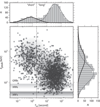
Figure 2.4. The spectral-duration distribution of GRBs as seen by BATSE. The scatter plot of E_peak versus T₉₀ shows two clear loci of events (shaded regions) with shorter events appearing preferentially harder (i.e., larger E_peak). The approximate E_peak distribution of XRFs, XRRs, and GRBs is shown as horizontal gray regions. The outset histograms, showing the number of events in a certain parameter range (top: duration; right: peak energy) also show a separation (most prominently in duration). The smooth curves atop the histograms show representative log-Gaussian fits to the distributions. The traditional two-second dividing line between “short” and “long” GRBs is shown. While the bimodal distribution in duration persists across instruments, a plot of hardness versus duration for Swift-only GRBs would appear differently: since Swift is relatively insensitive to detecting very hard events of short duration and very soft events at long duration, there is no clear bimodality in hardness of Swift events. The uncertainties in the measured quantities for each event are not shown for clarity. I am grateful to Nathaniel Butler who kindly provided the E_peak and T₉₀ fits to the BATSE data.

Finding trends and relationships between observables is not only an important trait for human survival,¹¹ but it is also an important platform in making sense of an otherwise large melee of metrics on phenomena we care about. Indeed, taxonomy in science is not just stamp collecting but a bona fide tool useful in uncovering the physical relationship between members. The duration-hardness distribution (figure 2.4) serves as the backbone for GRB taxonomy. These two parameters are among the most easily observed in an event, and they clearly have the power to distinguish two broad classes of events.

As discussed in chapter 1, long-duration soft-spectrum GRBs (LSBs) have been associated with the death of young massive stars, while short-duration hard-spectrum GRBs (SHBs) have now been associated with an older stellar population. So, at first blush, it would seem that this high-energy classification may indeed reflect a significantly different physical origin of the events. There are complications, however. First, even after accounting for various observational biases, ascribing membership of a given event to one class is inherently probabilistic since there is clearly a broad overlap between phenomenological classes (figure 2.4). A burst lasting one second certainly could belong to the tail end of the “long” class, while a burst lasting ten seconds could properly belong to the “short” class. Second, the same burst observed at different redshifts will have a different observed spectra and T₉₀. In particular, an SHB occurring at high cosmological redshift could easily manifest itself as an LSB. Likewise, some long-duration bursts with an overall soft spectrum could have a short/hard initial pulse. If faint enough, the long/soft portion of the burst could be lost in the detector noise, making the source seem like an SHB. Last, there appear to be many individual events from within the Milky Way and other nearby galaxies that could easily have been classified as an LSB or SHB based on high-energy properties alone but that arise from very different progenitors^* than the majority of the events.

Whether the high-energy properties of GRBs can directly reflect the progenitor diversity is a question we will revisit in §5.4. The progenitor question as it relates to observables is, in some sense, like asking about the properties of performers singing in a chorus. Are all baritone parts sung by men? Is someone’s degree of vibrato correlated with his/her age or with the part of the world he/she was born in? Irrespective of such inquiries, we can ask what is the physical origin of the sound and voice itself, or, in our case, what is the physical origin of the light of GRBs.

2.2 Understanding the Origin of the High-Energy Emission

What is seen in the first moments of a GRB is commonly referred to as the “prompt emission”; as shown previously, most of the prompt energy is in the form of gamma rays. During the GRB itself, roughly 0.1 percent of the restmass energy of the Sun is thought to be radiated away in gamma rays alone. The spectra and light curves of GRBs provide vital clues to frame our understanding of the events. For instance, since gamma rays are a natural consequence of radioactive fission decay, it is reasonable to ask whether GRBs are due to such decay. Setting aside the challenges in arranging an event where so much energy is released from radioactive decay, this scenario is ruled out since we do not see evidence for fission-process gamma-ray lines in GRB spectra. Moreover, the light curves are not consistent with what is expected from radioactive decay.¹² What if, like in supernovae, the energy of the radioactive material was captured by the material in the explosion itself? In technical terms, we would say that the material had high optical depth^* to the absorption of gamma-ray light. In this scenario, we could expect to wash out the gamma-ray lines, and the energy otherwise carried in those lines would heat up¹³ the absorbing material; this energy is then reradiated, usually at lower frequencies. The emergent spectrum of this reradiated energy would be expected to be that of a blackbody.^* Unfortunately for the vast majority (if not all) of the observed GRBs,¹⁴ it is not: bursts fit by a Band spectral shape are too bright at high energies and too faint at low energies to be consistent with a blackbody.

2.2.1 Compactness Problem and Relativistic Outflow

That GRB spectra are not consistent with blackbody emission implies that, at gamma-ray energies, the emitting system is optically thin (i.e., τ < 1). This turns out to be a major constraint on the nature of the material that participates in the radiation. The most important part of this clue is the recognition that many high-energy gamma rays (well above E_peak) have escaped the source despite the propensity of gamma rays to interact with other photons and produce electron-positron pairs. Such pair production is only possible when, in the center-of-momentum frame of the two photons, there is enough energy to produce two particles of the mass of an electron (m_e); that is, when the available energy is comparable to 2 × m_ec² = 1022 keV ≈ 1MeV.¹⁵ The optical depth for a high-energy photon escaping from a spherical system (with an appropriate number of low-energy photons around to pair-produce with) is:

where σ_T is the cross-section for the interaction of photons with other photons to produce electron-positron pairs,l is the length of the material through which the high-energy photon travels, and n_γ is the volumetric density (units of [length⁻³]) of low-energy photons for which the pair-production energy threshold is satisfied.^* The number of suitable photons (N_γ) should be something comparable to the total energy of a pulse in gamma rays (E_pulse) divided by the typical suitable photon energy (~m_ec²); the number density n_γ is just N_γ divided by the volume (4 π l³/3). As in §1.4, we can employ the 1/r² law to estimate energy from the inferred distance (d) to the source and the fluence (S_pulse) of a pulse. This yields an estimate for the optical depth of:

For a cosmological GRB, we can assume a rough distance of d ≈ few Gpc and a typical pulse fluence of S_pulse = 10⁻⁷ erg cm⁻². Recalling the light-travel time argument from §1.4, we can infer from the variability timescale of a GRB (δt ≈ 0.01 sec) that the size of the source responsible for emitting the energy in a single pulse should be of length l c δt ≈ 3,000 km. Putting in the numbers, we infer that the optical depth to pair production is τ ≈ 2 × 10¹⁴; with a number this large, we should see no high-energy gamma rays at all! Some assumption in our calculation must have been seriously wrong—the source appears to be much too compact (small l) to allow the observed spectrum to emerge.¹⁶

The solution to this so-called compactness problem comes from the invocation of relativistic expansion of the radiating material. If the material is expanding at a rate close to the speed of light, then two effects work to diminish the true optical depth greatly. First, relativistic motion leads to extreme Doppler shifts of the intrinsic spectrum; a photon observed at tens of MeV might have been generated in the source at much less than a few keV. Thus, at the source, the number of photon pairs satisfying the pair-production energy threshold is greatly reduced. Second, a relativistically expanding source that is emitting can be much larger than the observed variability timescale would suggest. If the expansion velocity is v then when considering relativistic motion, it is convenient to introduce another parameter, Γ, derived from velocity called the Lorentz factor.^* The first effect reduces the inferred τ by roughly Γ^2β, where β is the Band spectral index after the peak (β ≈−3; see §2.1.1). The second effect arises because the emitter closely lags behind the light it just emitted, so the arrival time of successive pulses is bunched up for the distant observer.¹⁷ As will be discussed more fully in the footnote on page 62, a pulse emitted over a time δt’ (as viewed by someone traveling outward with the explosion) appears to last just δt = δt’/ (2 Γ²). Since the effective τ is reduced by Γ^2β−2/2, an optically thin GRB (τ < 1) requires (for the example values we used here) Γ 57. This implies that the material producing the GRB must be moving at least as fast as 99.985 percent of the speed of light! Amazingly, detailed modeling of some specific GRBs¹⁸ have given minimum Lorentz factors of Γ > 1,000.

Relativistic motion in other high-energy phenomena (e.g., the jets emanating from supermassive black holes) is not itself unusual, but the values of Γ inferred for GRBs are larger by an order of magnitude than any other studied phenomenon in nature. Less than two years after the 1973 discovery paper, Mal Ruderman reviewed the basic physical theories for the origins of GRBs.¹⁹ In this review, he noted how the compactness argument pushed the inferred Lorentz factor for GRBs at cosmological distances to uncomfortably large values, thus providing weak support for a Galactic origin. The Galactic origin, with a lower distance d, would require only mildly relativistic outflow (see equation 2.3). This is a common approach in science: take an idea (e.g., a cosmological origin for GRBs) to its logical conclusion and show its extreme nature—and, perhaps, absurdity—relative to a more simple possibility (i.e., a Galactic origin). But this weak support for a Galactic origin is actually a prime example of the failed application of Occam’s Razor. Unfortunately for both Occam and Galactic models, we have learned that GRBs do not shy away from extrema but instead appear to delight in confounding theorists and their intuition.

2.2.2 Fireballs and Internal Shocks

Well before the light of a GRB escapes, the outflowing material needs to accelerate to the relativistic speeds we infer. The basic picture (see figure 2.5) is that a significant amount of energy (which must be at least equal to the energy observed in the gamma rays) is rapidly deposited into a small region of space of size l ≈c δt. The source is compact (§2.2.1) with the energy density so high that gamma rays readily collide to make electron-positron pairs. These pairs readily annihilate to form high-energy gamma rays. Since most of the energy is held by the photons (as opposed to the entrained matter, like electrons and protons), we call this the “radiation-dominated” phase. By construction, this soup of particles and light (referred to as a fireball) is opaque: few photons escape; therefore, the energy is trapped.²⁰ Since there is nothing to confine the fireball, it expands. During the expansion, the energy associated with the internal random motions of the moving particles and gamma rays are converted into bulk outward flow. Basic conservation arguments—that is, requiring energy and momentum to be unchanging—show that the Lorentz factor of the expanding fireball grows linearly with the radius of the fireball.

Figure 2.5. The evolution of the Lorentz factor in a GRB as a function of radius from the explosion. Energy is deposited by the central engine at a radius of c δt (about the radius of Earth, ), and Γ of the fireball increases linearly with radius until a maximum Lorentz factor Γ₀ is achieved (at about the radius of the Sun, R). Internal shocks occur at r ≈ c δt, at about one astronomical unit [AU], and some energy is lost corresponding to a decrease in Γ (here we take the efficiency of conversion to gamma rays—see §3.2.1—to be η = 0.1). At a radius comparable to a fraction of a light-year, the blastwave begins to decelerate due to interactions with the external medium. It is during this external shock phase that the afterglows are produced (see §3.2).

Eventually all the mass (both in the form of electrons and protons) entrained in the fireball will hold all the energy, now in the form of kinetic energy. We say that the fireball is now “matter dominated.” Since the total energy²¹ of a relativistic particle with mass m is Γ mc², if ε is the total energy in the fireball and M_tot is the total mass, it follows that the fastest the material can flow is Γ₀ = ε/ (M_totc²). Once this “terminal Lorentz factor” (Γ₀) is achieved, the protons in the fireball are essentially moving outward on ballistic paths. We say that the fireball has now become “cold” because there is little random motion of the protons apart from their radial trajectories—if you were moving with the outskirts of the fireball, you would see almost no motion of neighboring protons toward you or away from you. The material coasts along with Γ₀ essentially unchanging over more than two orders of magnitude in radius from the explosion site. Since we have estimated that Γ of the flow around the time of the GRB must be greater than ~57, we can turn this around to estimate the mass of particles in the fireball to be M_tot ≈ 10⁻⁵M_, recalling from §1.7 that E is at least ~10⁵¹ erg.

An entrained mass M_tot that is more than three Earth masses may seem like a lot of material, but this “dirty fireball” is a rather pristine ball of pure energy—supernova explosions, in contrast, have hundreds of thousands times more mass taking part in the bulk expansion. If there was any more mass in the fireball, then the largest Lorentz factors would be diminished, which would violate the constraints from the observed spectrum.

If the fireball was expanding out into a vacuum, there would be no easy way to turn the kinetic energy of outwardly flowing particles into the radiated energy we see. The most basic requirement is that the particles that carry the kinetic energy must be perturbed away from their outward trajectories. The simplest possibility on the path to energy release—like a car hitting a brick wall—is to have outflowing matter (mostly electrons and protons) smash into stationary material (atoms, electrons, protons, etc.) in the surrounding material. However, the density of matter in the outflow and the density of surrounding material are so low that direct interactions at the atomic level²² are very unlikely. Like ships passing in the night, there is simply too much space for such collisions/scatterings to take place. Instead, long-range forces must connect the particles, allowing them to transfer energy and momentum to each other “collisionlessly.” Magnetic fields (near the edge of the fireball) are thought to be this mitigating glue.

When energy and momentum are transferred from particles in one fast-moving region to another, a shockwave is generated. We think of shocks as discontinuities in the bulk properties of one region with another (such as density, temperature, and pressure). The discontinuity remains sharp (i.e., abrupt changes over a small range in distance) because the outflowing matter is moving faster than the news of the disturbance itself can move in the material upstream from the shock. For airplanes moving faster than the speed of sound, the shock gives rise to a sonic boom. For GRBs, relativistic (collisionless) shocks are the places where kinetic energy associated with outflow is transferred and that energy is radiated (we discuss radiation from shocks in §2.3.3); with GRBs, in effect, we see the cosmic boom.

There are two possible origins for the creation of such shocks. First, the outflowing mass may run into material around the explosion site (circumburst medium [CBM]), causing it to slow up; in slowing, some of the outward kinetic energy is then transformed into random motion of the particles, which, in turn, can be effective at radiating light. Second, the outflowing fireball could catch up with another outflowing shell of material and merge with that shell. Conservation of linear momentum, energy, and mass then dictate just how much the sum of the kinetic energy in the two shells could be available to radiate away. The former, referred to as the external-shock scenario,²³ is attractive because of the efficiency in converting bulk flow to radiated energy, but it has a serious problem explaining the near-constant width of pulses throughout the gamma-ray light curve of the GRB. In the external-shock scenario for the prompt emission, the observed variability of the GRB comes from a clumpy circumburst medium. The latter scenario (of shells of material catching up with other shells) is known as the internal-shock scenario²⁴—it can easily explain the complex light curves of GRBs, but the efficiency of turning outward kinetic energy into random motions of radiating particles is low. This implies that ε must be much larger than the energy released in gamma rays. In this scenario, the observed variability comes from the diversity of energy and Lorentz factors of shells emitted at the source. The internal-shock scenario has emerged as the most likely explanation for the conversion of the kinetic energy of the outflow that gives rise to the prompt emission; the external-shock scenario is the favored mechanism for the generation of GRB afterglows.

2.3 The Central Engine

In the internal-shock scenario, the number of pulses we see is roughly equal to the number of fireballs created by the energy source at the center of the explosion, the so-called “central engine”. Likewise, the duration of the GRB directly reflects the lifetime of the activity of this engine.^*

We have never actually seen the central engines of GRBs directly, but we can infer some basic properties of them. First, the central engine must be capable of sporadically dumping 10⁴⁸–10⁵¹ erg of nearly proton-free energy into a volume comparable to that occupied by Earth. Second, some engines must live for at least tens of milliseconds (to account for the shortest bursts) and some for thousands of seconds. Last, since the total energy output in gamma rays is about the same for the majority of GRBs we see (cf. chapter 4), there must be some common properties among the engines for different observed GRBs. However, since every GRB has a different light curve, every engine must also be active in its own way.

The energy budget and volume constraints quickly whittle down the possibilities to compact objects, suchas neutron stars (mass ≈ 1 M; radius ≈ 10 km), black holes (mass ≈ 10 M; radius²⁵ ≈ 30 km), and white dwarfs (mass ≈ 0.5–1.4 M; radius ≈ 3,000 km); all other possible culprits (e.g., stars like the Sun) are incapable of releasing so much energy in so little space. While a variability timescale of tens of milliseconds is a natural consequence of the small sizes, the tens-of-seconds durations (recall that these durations must reflect the time that the engine is active; see footnote on page 62) are much longer than the light- or sound-crossing time for these objects. Thermonuclear explosions involving white dwarfs and neutron stars (e.g., novae and supernovae) certainly progress on longer timescales, essentially set by the time it takes for the system to become optically thin. But those explosions are very “dirty” (i.e., too much mixing of protons in the expansion), and any short-timescale variability is generally washed out in such events.

Instead, a different sort of central engine must be responsible for powering GRBs. We now take a tour of the various possible central engines, examining the expected characteristics of the resultant events.

2.3.1 Accretion-powered Events

One scenario that explains both the timescales and energies posits that the energy source ultimately comes from mass inflow into the central engine. The “best bet” scenario²⁶ for this form of central engine goes something like this: because of some catastrophic event, mass at large distances starts flowing toward the central compact object. Generically, inflow toward a central mass is called accretion. At large distances from the central source, this inflowing mass holds an appreciable gravitational potential energy that is then converted to kinetic energy during the flight inward. If the mass initially has even the smallest amount of motion tangential to the direction of the compact source, it will swirl inward rather than plunge directly. You should be picturing water flowing down a drain rather than hail (or meatballs) raining down toward the ground.

If there is an overall rotation to the matter before inflow begins, a disk of swirling mass will form. There will be friction within this accretion disk, which serves to heat up the material in the disk and speed the rate of inflow. Some of the original potential energy of the material can be tapped in two ways: (a) the fast-moving electrons can generate strong magnetic fields with high energy densities, and (b) energetic neutrinos can be produced in the disk and flow away from the source. These processes of energy extraction are not steady and thus naturally could explain some of the observed variability. As long as mass continues to flow inward, some of the potential energy becomes available as an energy source.

It is interesting to examine the efficiency (η) of the potential-to-kinetic energy conversion for various central engines based on accretion. This efficiency yields a formula for the maximum energy release via accretion of this type of central engine: E_max = ηMc², where M is the amount of mass flowing toward the central source. To calculate η, we calculate the potential energy difference for some mass m as it moves from a very large distance r_large to the (effective) edge r_edge of the central source as a fraction of its restmass:

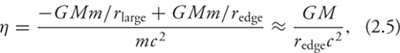
where M is the mass of the central object and the approximate solution comes from assuming that r_large r_edge. A solar-mass white dwarf (WD) has a radius of about 5,000 km, so η_WD ≈ 3 × 10⁻⁴. A neutron star with mass 1 M has a radius of ~10 km, so η_NS = 0.15. A nonrotating black hole has η_BH = 0.06; a fast-spinning black hole can have η_BH = 0.42. In contrast, nuclear-fusion processes have a maximum efficiency of just η = 0.007, twenty times less than that of a neutron star. It is clear from this analysis that WD (nuclear-driven) events are at a severe disadvantage in their ability to liberate accretion-derived energy—for the same overall efficiency of conversion of restmass to observed gamma rays, WD (nuclear-driven) events would need to involve > 200 (> 23) more mass than that required if the central engine were a black hole or neutron star. Since the total energy liberated in just gamma rays (which is bound to be just the tip of the energetics iceberg, as we shall see later) is E _γ ≈ 10⁵¹ erg ≈ 10⁻³ M c², the total mass involved must be of order at least a fraction of a solar mass.

2.3.2 Centrally Powered Events

Alternatively, if the central source is a newly forming neutron star, significant energy can be tapped from the gravitational contraction of the proto-NS itself. The heat generated from this contraction is radiated away as hot neutrinos, some of which interact with the protons and neutrons around the source and can drive a powerful wind. The significant energy associated with the rotation of the NS could also be tapped through interactions with large, nascent magnetic fields.^* Assuming the NS is a perfect sphere, the rotational energy ε_rot available initially is

where P is the initial spin period of the NS. This period is thought to be very high (P on the order of milliseconds). Typical numbers yield ε_rot ≈ 2.2 × 10⁵² erg. Detailed calculations²⁷ show that magnetic fields can dissipate this energy at large distances from the central source and accelerate matter to high Lorentz factors. The resultant outflow would be highly magnetized, which could have direct observational consequences, such as highly polarized prompt emission (see §2.1.1).

2.3.3 Energy Dissipation: The Origin of the Prompt Emission

Up to here we have summarized the engines and bulk processes that could make enough energy available to be radiated, but we have not discussed how this energy is radiated. Radiation is expected when a charged particle (e.g., an electron or proton) is accelerated (or decelerated)—generically, some of the available free energy that is used to accelerate the particle is carried away from the system by the emitted light.^†

Recall that the hot fireballs of energy and plasma (ionized gas) eventually expand, converting thermal (random internal) energy into bulk kinetic outflow at relativistic speeds. If the energy is deposited episodically for the duration of the GRB, each fireball will stream away with its own bulk Lorentz factor, magnetic fields, total energy, and entrained mass. Viewed from afar, the outflow looks like a relativistic wind.

When (and if!) a faster-moving shell in the relativistic wind catches up to a slower one, rather than sail right through unimpeded, the faster shell is slowed up as it begins to merge with the slower shell. A collisionless shock (§2.2.2) is established between the two shells. Viewed by the inner (faster-moving) material, the particles in the outer shell appear to be raining inward at a velocity comparable to the difference of the velocities of the inner and outward moving shells.^* Upon entering the shocked region, these particles (electrons, protons, and neutrons) are deflected from their radial trajectories. This deflection provides internal thermal energy that now becomes the primary energy deposit that can be tapped and radiated away.

In analogy to observations of nearby supernova (nonrelativistic) collisionless shocks, we believe that the observations of GRBs are consistent with a population of electrons that are accelerated to relativistic speeds within these shocks. The basic idea, called “Fermi acceleration,” is that charged electrons enter the shocked region and are “reflected” by magnetic fields within the shock serving to boost their kinetic energy incrementally. After multiple reflections, the electrons have gained a considerable amount of energy and can move at speeds much larger than the outward speed of the shock itself. Fermi acceleration theory posits that an ensemble of such magnetically reflected electrons will take on a powerlaw distribution in energies. Indeed, as in supernovae shocks, there is reasonable evidence from afterglow observations (see §3.2) that most of the energy in the fast-moving electrons is distributed into a powerlaw distribution of electron energies such that, for every factor of ten increase in energy, there is about a factor of 150 fewer electrons.^* Though Fermi acceleration theory is attractive, there are a number of ad hoc assumptions²⁸; in truth, for supernovae and GRBs alike we do not understand precisely why the electrons are accelerated into a powerlaw distribution in energy and why the precise value of that powerlaw might be different from event to event.

The total energy now imbued into these fast-moving electrons might be a few percent of what was once the total kinetic energy of the shell. However, these electrons could not, on their own, easily radiate away their potent stockpile of energy: they must either accelerate or decelerate to produce light.²⁹ In the presence of a magnetic field, the trajectory of moving electrons is curved, which causes them to accelerate. When the electrons are moving near the speed of light, the light emitted by bending electrons is called synchrotron radiation. The electrons may also decelerate by interacting with a nearby photon: the electron serves effectively to scatter the light and impart some of its kinetic energy to the incoming light. The net result in this process called inverse Compton (IC) scattering is that the energy of the outgoing light is higher than that of the incoming light, at the expense of zapping the electron energy. The ratio of the amount of energy dissipated by synchrotron radiation and IC scattering is related to the energy contained in the magnetic fields relative to that in the photons in the shock.

These two emission mechanisms are the leading processes by which the few percent of the required shock kinetic energy in GRBs may be radiated (both for internal and external shocks). Unfortunately, the calculation of the emergent spectrum depends on a number of effects that are difficult to determine from first principles, such as the detailed electron energy distribution and the magnetic field strengths in the shocks. Still, with reasonable prescriptions, the basic spectral properties of GRBs appear to be reasonably fit by a blastwave emitting through synchrotron and IC. The detailed diversity of spectra among different GRBs (and during a given GRB) is not a generic prediction of a larger model but instead reflects real physical differences that are not readily calculated. Of course, performing fits of the observed data to theoretical models yields direct insight into the magnetic fields, electron spectral indices, and Lorentz factors. In this respect, GRBs are wonderful laboratories to study the microphysical properties of matter and energy in extreme situations.

 

^*For the purposes of this discussion, we will take high-energy emission to be any light observed with photon energies larger than 10,000 electronvolts (eV)—that is, energy in the X-ray and gamma-ray portions of the electromagnetic spectrum.

^*This is referred to as fluence and has units of energy per collecting area. Mathematically, fluence is the integral of the light curve flux over time.

^*For example, magnetars. See §5.3 for an extended discussion.

^*Optical depth, usually symbolized as τ, is a dimensionless number describing the stopping power of matter to light at a certain wavelength of light. Physically, the intensity of light going through that matter is decreased by a factor of e^−τ (the value e = 2.718... is called sometimes referred to as “Euler’s number”). Your body has a high optical depth to visible light but low optical depth to, say, radio waves. The reason X-ray scans of your body work is that materials of different composition, densities, and sizes all have different optical depths so the number of X-rays that penetrate to the film will vary through different sightlines.

^*A blackbody, or thermal, radiator has a spectrum that is entirely characterized by the temperature of the material. Theoretically, a blackbody is a perfect absorber (i.e., it does not reflect light, τ → ∞) at all wavelengths and, because it would have to be in thermal equilibrium with another blackbody attached at the same temperature, must also radiate the energy it absorbs (so as not to heat up). The peak in a blackbody spectrum is linearly proportional to the temperature of the source. People are not good blackbodies at optical wavelengths, and we know this because we reflect the ambient light in the room. But we do radiate like a blackbody near the peak of our spectrum—at mid-infrared wavelengths, around 10 µ m, dictated by the internal temperature of our bodies.

^*Here, think of τ as related to the probability that a high-energy photon will pair-produce at some point while it traverses the region where other photons are present. Though light and electrons do not have physical size per se, it is instructive to think of a cross-section as an effective two-dimensional size. If the cross-section (in units of area or [length²]) is large, then more reactions can occur because there is a higher chance of one photon interacting with another. Likewise, there will be a high optical depth if the density of interacting particles is larger or the photon traverses a longer path. An apt analogy would be trying to calculate the chance of your bumping into someone if you ran down a long school hallway with your eyes closed. That chance is low between classes when the density of other students in the hallway is low. But for the same density of people in the hallway,τ will be higher if everyone is an oversized football player (high cross-section), and τ will be lower for a bunch of diminutive kindergardeners (low cross-section). Please do not try to reenact this thought experiment!

^*Formally Γ = . When v is 99% the speed of light, Γ = 7.09. Likewise, Γ = 100 for v = 0.99995 × c. The Lorentz factor can take on any value greater than or equal to 1 (v = 0). A fast supernova explosion has Lorentz factors of ~1.001–1.003.

^*In a relativistically expanding system, the time of events as viewed by distant observers appears to be compressed heavily relative to an observer sitting at the center of the event; indeed, if the evolution of a GRB was a ninety-minute soccer game for fans in the stadium, those of us watching at home would see everything happen in a fraction of a second. Consider two photons, one released toward a distant observer at radius r₁ and another released when the expanding source, traveling with velocity v, has reached a larger radius r₁ + δr. The photon released from r₁ will arrive at a time δr/v − δr/c before the photon released at radius r₁ + δr. When Γ is very large, a little algebra shows that the relation ≈ is approximately correct. Thus, the observed time difference between the pulses is

Since the blastwave is moving at very nearly the speed of light, events that happen at time t as viewed by the center of the explosion (r₁ = 0) occur at radius δr = ct. Thus, we find that time is “compressed” for a distant observer (relative to the time measured at the explosion center): . Now imagine that we have two shells of mass traveling with Γ₂ > Γ₁ with shell 2 emitted after a time δt as viewed by someone at the center of the explosion. Eventually shell 2 (with Γ₂) will catch up with shell 1 traveling at a slower speed. If Γ₂ is a factor of a few larger than Γ₁ then one can show that the two shells collide, producing the GRB (see §2.3.3), at a distance δr = c δt Γ₁ Γ₂. From equation 2.4, it is then clear that t_obs ≈ δt. That is, even though there is strong time compression of events, the observed duration in GRBs directly reflects the time that the central engine was active.

^*The rotational energy of a spinning BH can also be extracted via magnetic fields in the so-called Blandford-Znajek process.

^†We also expect light to be emitted when an atom—which can temporarily act like a microscopic battery by storing energy—relaxes to a lower energy state. In the case of GRBs, as we now describe in this section, the former channel is expected to dominate.

^*Since both velocities are relativistic, a formula for relativistic velocity subtraction must be used. The result is that the inner shell will see relativistic velocities of the inflowing material at a Lorentz factor somewhat less the Γ of the outer shell.

^*We can write the differential number density distribution of electrons at some energy E as:

where p is the “electron spectral index” (usually determined in afterglows to be about p ≈ 2.2 and where the constant is determined such that the integral of E over all energies gives the total energy in electrons). Evidence from radio observations suggests that this powerlaw distribution of electrons actually has a low-energy cutoff at around E_lower ≈ m_ec², where Γ is the effective Lorentz factor of the incoming shell as viewed by the faster-moving shell.