4

THE EVENTS IN CONTEXT

L’accent du pays où l’on est né demeure dans l’esprit et dans le coeur, comme dans le langage.
[The accent of one’s birthplace remains in the mind and in the heart as much as in one’s speech.]

—François duc de La Rochefoucauld,

Maxim 342, Réflexions ou sentences et maximes morales

(Reflections; or Sentences and Moral Maxims), 1664

Prompt and afterglow emission of GRBs are largely driven by the central engine behavior, the explosion properties, and the physics of relativistic shocks. Those seconds, minutes, and days after the main event tell a remarkable story about how the progenitors of GRBs end their life. But it is the context—where GRBs occur inside and out of galaxies and throughout cosmic time—that tell us how the progenitors lived. Indeed, we treat GRB locations like a crime scene, extracting forensic evidence to make a case about the lifecycle of a GRB progenitor; that progenitor, while on the other side of the Universe, would one day get a bunch of astronomers on Earth scurrying around to make sense of it all.

4.1 Local Scales

4.1.1 Circumburst Environments

X-ray absorption and emission lines (§3.1.1.1) in long-duration GRBs were suggested to arise from a very specific (and somewhat contrived) geometry of the circumburst medium (CBM). Had these spectral features been found to be real, a dense patch of gas-phase metals at 10¹⁷–10¹⁸ cm from the burst would have been required. This, in turn, would have given a rather specific view of the history of the amount of material expelled (“mass loss”) by the progenitor. Instead, since the significance of the X-ray diagnostics has remained low, we are forced to turn to other approaches for inferences about the CBM. We saw in §3.2.1.2 that, modeling caveats aside, GRB afterglows can be used to infer both the density of the CBM as well as its change with distance r from the explosion site. We can parameterize the density of the circumburst medium as ρCBM = C × r ^s, with C as some constant. All other parameters being equal, the larger the value of C, the brighter the afterglow will be. As we have seen, the values of C and s also affect the dynamics of the blastwave. The smaller the value of s, the longer the blastwave will travel at relativistic speeds. A homogeneous (uniform) medium has s = 0 and C = n × m_H. This is the nominal expectation of a burst that occurs far from the influence of stars, in the interstellar medium (ISM)¹ or in the intergalactic medium (IGM). Typical values for the ISM and IGM are, respectively, n_ISM = 1 cm⁻³ and n_IGM = 10^{− 6} cm^{− 3}. If instead the progenitor is a dying star, we expect a different value of C and s. The simplest assumption is that this star should shed its outer envelope as a stellar wind, much like the Sun does but with more mass and at faster velocity. Assuming a constant velocity and constant massloss rate,^* one can show that s = −2. Such a “windblown” CBM (§3.2.1) is the most obvious expectation for a GRB that originates from a massive-star explosion, especially one that also produces an SN: massive stars are observed to have very strong winds giving rise to ρ r ⁻² density profiles in massive-star SNe observed in the local universe. Yet, with model fits to observations, a constant density medium (s = 0) is preferred in the overwhelming majority of long-duration GRB afterglows.^† For the few short-duration GRBs that have had enough data to model C and s values, there appears to be broad consistency with a homogeneous s = 0 medium. In many cases, there is an indication that C is significantly less than seen in long-duration GRBs; the implications of this will be discussed in §5.2.

Since the majority of long-duration GRBs are thought to come from the death of massive stars (§5.1), the s = 0 environment is a considerable bugaboo. Least favored, but certainly not out of the question, is the notion that our physical model of the afterglows is really incorrect and that we actually are not measuring s at all. Another possibility is that GRB progenitors are not like the sort of massive stars we observe in the local universe; still, it would be a highly contrived situation if the massive stars all had special massloss histories that mimicked an s ≈ 0 environment. The current consensus is that the environments around many GRBs are homogeneous but that this homogeneity derives from an interplay between the outflowing wind of the progenitor that has interacted strongly with the interstellar medium and/or the remains of the star-forming region that harbors the progenitor. This idea also has its problems: the s = 0 medium appears to exist so uncomfortably close to the explosion site (at least as close as 10¹⁶ cm, where the afterglow starts radiating) that the external medium would need to be very dense (> 10⁴ cm⁻³) to create such a homogeneous bubble. The CBM homogeneity issue, without a truly satisfying explanation, persists.

Another useful vista into the circumburst environment is to look for time-dependent changes that are attributable to interactions of the afterglow light with the material around the GRB event. Here the composition of the circumburst medium is important (not just the density). In the case where there are just atoms in the CBM, the atoms that are in our line of sight to the afterglow will absorb the afterglow light (§3.1.2) at specific wavelengths. These wavelengths (and depth of absorption) depend on the specific population of electrons bound to the atoms and the quantum-mechanical rules that dictate how those electrons can gain energy by absorbing an afterglow photon. Near the GRB (say within 100 pc), these atoms are bombarded by the deluge of afterglow photons at such an appreciable rate that one can show that, within a few seconds, essentially all the electrons of all the atoms are stripped off, leaving a fully ionized plasma of nuclei (protons + neutrons) and free electrons. If there are any simple molecules in the CBM (such as H₂ or carbon monoxide), then these too should be shredded by the afterglow light. Dust particles are complex molecules (or “grains”²), but these too can be destroyed by a number of photon-interaction processes. The GRB perpetrator is rather adept at wiping clean the crime scene.

Dust destruction almost certainly happens around a GRB, but no unambiguous case for dust destruction has been seen in the time variability of an early afterglow.³ Aside from a high-ionization line of nitrogen, there are no atomic absorption lines that are attributable to atoms in the CBM—again, not that the atoms are not there, just that they are fully ionized before we can acquire a spectrum of them.⁴ Also consistent with the general picture is that most GRB afterglows do not show evidence for molecular absorption, despite the fact that the star-forming regions in the Milky Way do harbor simple molecules. The notable exception is the long-duration GRB 080607, which showed significant absorption due to H₂ and carbon monoxide.⁵ What set this event apart from most others is that there was a considerable amount of dust along the line of sight—perhaps the largest amount ever seen in a GRB—and that the afterglow was intrinsically one of the brightest ever inferred. This, combined with the fact that we were able to observe the event at moderately high spectral resolution quickly (within about ten minutes) on a large-aperture telescope, allowed the molecules to be observed in absorption. Though the cloud housing the molecules was reckoned⁶ to be more than 250 pc from the GRB site, these afterglow observations of GRB 080607 provide the best evidence to date for a nearby environment similar to star-forming molecular clouds studied in the Milky Way.

4.1.2 Subgalactic Scales

From a progenitor perspective, the lack of telltale diagnostics of the CBM in all but a few cases is disappointing but entirely reasonable. To be sure, there is significant absorption (both broadband and in narrow lines) in long-duration GRB spectra that is attributable to the absorption nearer to the GRB than to us. However, aside from the few cases mentioned in §4.1.1, the absorption sites are thought to be in physically disconnected regions in the host galaxy (that is, far away from the GRB). GRB afterglow light pierces through random sightlines in its host galaxy, so if it encounters a pocket of dust or gas, those distinct places within the host galaxy will leave their distinct imprints on the afterglow. The only difference with CBM regions is that, because of the distance from the GRB, there are not enough afterglow photons to do any destructive (ionizing) damage. In a few well-observed cases of long-duration GRBs,⁷ we have been able to witness the changes of atomic states as a function of time. In such events—observed in the few minutes to hours following the GRB—there are enough photons to alter the states of some ions at hundreds to thousands of parsecs from the GRB site. After the afterglow fades, some atoms relax back to their original states. By observing the rate of depopulation and repopulation of some states, one can infer the distance of the absorbing cloud from the GRB and, in addition, some basic properties of the cloud (such as density). When such data can be obtained, we get a delicious upfront and personal view of random clouds in distant galaxies in a way not possible by other means. For astronomers, it is like anonymously following the Twitter stream of a random person in a far-away country for long enough to learn about his/her community and what makes him/her tick.⁸

The vast majority of long-duration GRB afterglows observed spectroscopically do not show time-variable behavior in the absorption lines. Yet at high spectral resolution, it is clear that persistent absorption lines arise from the light of the afterglow passing through distinct clouds in the host galaxy.^* We can separate the clouds by looking at slightly different wavelengths. Motion within those distant galaxies—individual clouds having slightly different speeds moving toward and away from us—gives rise to distinct Doppler shifts such that their atoms appear to absorb at slightly different wavelengths. In each cloud, we can see the relative amounts of atoms in different states of ionization. In many cases we can also determine the total amount of hydrogen in the host galaxy.^†

Measuring the amount of metals^* relative to the amount of neutral hydrogen gives us a sense of how much of the ISM of that galaxy has been enriched by synthesized (heavy) elements. We usually compare this measurement to the same measurement made in the spectrum of the Sun, deriving a value called metallicity. GRB afterglows have allowed us to make dozens of metallicity measurements in GRB hosts. In general, the metallicities inferred are less than that in the Sun. In the very distant universe this is not entirely unexpected, given that the GRBs are formed from stars that themselves have formed before significant amounts of metals have been spewed out from SNe.⁹ One very interesting result is that, in the few GRBs that have occurred “nearby” (within one billion light-years from Earth), the metallicities inferred for those GRB hosts (and, in particular, at the very location within the host where the GRB occurred) tends to be much lower than seen in a typical nearby galaxy.¹⁰ This is taken as evidence that the progenitors of long-duration GRBs prefer low metallicities for their formation. No absorption spectrum of an unassailably classified short-duration GRB has been acquired to date. The utility of measuring metallicities in GRBs, apart from inferring something about the progenitors, is discussed in §6.1.

4.2 Galactic Scales

Bright afterglows are wonderful for probing gas and dust in absorption: we need a lot of light at all wavelengths to be sure which photons are missing at which wavelengths.¹¹ But since afterglows can be millions of times brighter than entire galaxies until they fade, trying to capture an image of the large-scale environment around a GRB is as futile as snapping a picture of a firefly in front of stadium lights.

When the afterglows do fade, we can determine where within (or outside) galaxies the events occur. In the special cases of the most nearby GRBs, the galaxies are big enough on the sky that we can image and study the specific locations of the events with imaging resolutions^* of tens of parsecs, comparable to the size of large star-forming regions. In the case of long-duration GRB 980425 and SN 1998bw, the event occurred within a cluster of stars in the spiral arm of an otherwise normal-looking galaxy. This cluster was less than 1 kpc away (but physically distinct) from the most copious factory of massive stars in that galaxy. A few other low-redshift GRBs (e.g., 060218 and 060505) also appeared to be associated spatially with ongoing and vigorous star-forming regions in the parent galaxy.¹² However, for the overwhelming majority of GRBs (both of the long and short varieties), the GRBs are far enough away from Earth that even the sharpest imager (such as the Hubble Space Telescope) cannot resolve the subgalactic structures to any less than a few kiloparsecs. We are, therefore, left to study the locations of GRBs in and around galaxies and the aggregate properties of those associated galaxies.

4.2.1 Locations

Less than one year into the afterglow revolution, the few long-duration GRBs that had been well localized via optical and radio afterglows proved very important for revealing which sort of neighborhoods they preferred and which sort of neighborhoods they avoided. Precise localizations¹³ told us that GRBs were not coming from the centers of galaxies, as one might have expected if they were due to activity around the central massive black hole found in most galaxies. Nor were these long-duration GRBs far from their apparent hosts, in seemingly empty space. Instead long-duration GRBs preferentially occurred embedded in the light of distant galaxies. The quantitative connection with galaxy light—and particularly blue galaxy light—in many individual cases could not be shown precisely, but larger samples showed a strong statistical connection with the ensemble. What location studies of long-duration GRBs did for the community was rule out some progenitor models, leaving models closely connected to the life and death of stars as the most viable.

Once Swift began localizing short-duration GRBs, locations became similarly useful in narrowing down the progenitor culprits of that class. But, since short-duration afterglows are generally fainter than those from long-duration events, the low success rate of measuring precise locations (with optical or radio afterglow) hampers the ability to make definitive statements about associations with host galaxies.¹⁴ Still, some short-duration bursts appear very clearly connected to the light of individual galaxies (which themselves tend to be blue, like the hosts of long-duration GRBs), and some appear to occur at large distances from their apparent hosts. There is good evidence that short-duration GRBs are more diffusely positioned about galaxy light than long-duration GRBs (which appear concentrated with the light of their hosts). However, the precise radial distribution of short bursts around their hosts is a difficult and uncertain practice (§5.2.3).

4.2.2 Host Properties

In almost all long-duration GRBs, the host associations are unambiguous, so we have a good deal of assurance that our study of those galaxies reflects the true population of GRB hosts. Long-duration hosts tend to be some of the bluest and faintest galaxies observed in distant galaxy studies. With only a few exceptions, they are also smaller in size than the Milky Way. The shapes (“morphology”) of those well-imaged hosts do not look like typical spiral galaxies (like Andromeda or the Milky Way) nor egg-shaped elliptical galaxies (like M87). Instead, the hosts of long-duration GRBs are usually characterized as being “irregular,” without clear morphological structure and, in many cases, without even an obvious center (see figure 4.1). The size encapsulating 95 percent of the star light is typically a few kiloparsecs and always less than 10 kpc.^* The closest analogs to GRB hosts we have in the local universe are dwarf satellites galaxies of the Milky Way, the Large and Small Magellanic Clouds.

Since the aggregate spectrum¹⁵ of newly forming star clusters is blue (as opposed to red for a group of old stars), the colors and brightnesses paint an important picture of GRB factories: at the time of the GRB, such birth sites are producing copious amounts of stars and yet have not produced an appreciable number of stars in the past. With high-quality images of the host galaxies in a number of optical and infrared bandpasses, the spectralenergy distribution (SED), coupled with models of how stars evolve with time, can be used to infer a total mass of the galaxy in stars. In accordance with their small sizes, the inferred masses are all less than that of the Milky Way and comparable to that of the Magellanic Clouds.

Spectroscopically, we can study in detail the emission lines from the hosts. Emission lines, like absorption lines, are due to specific transitions within atoms and can be used as a sensitive diagnostic of the conditions of star formation. Though there is a big range, we infer that star formation in GRB hosts is comparable to that in the Milky Way;^† but, since GRB hosts are ten-to-one hundred times less massive than the Milky Way, they appear to be very efficient producers of new stars given their relatively puny sizes. The small size and blue colors of GRB hosts suggest low metallicities (less than Solar abundances); this is in accordance with the low average^*metallicities in GRB hosts that are inferred using emissionline diagnostics. Interestingly, in the local universe, the metallicities of long-duration GRB hosts are systematically lower than in those hosts of observed SNe, suggesting some preference of GRB progenitors to be formed in lowmetallicity environments. At higher redshifts—above z > 1 when the average metallicity in the Universe was lower—the metallicities of long-duration GRB hosts inferred from absorption-line spectroscopy is similar to the metallicity inferred in the generic population of galaxies. Overall it seems that long-duration GRB progenitors are less likely to be formed at high (i.e., roughly Solar) metallicity. We discuss some interpretations of this conclusion in §6.1.

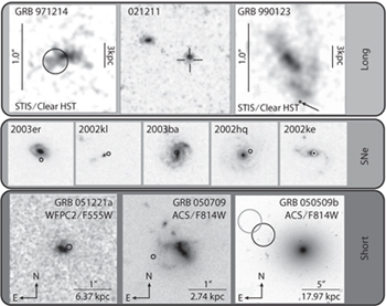
Figure 4.1. Gallery of GRB and SN host galaxies as observed by the Hubble Space Telescope. (top) Images around the locations of three long-duration GRBs with the position (and uncertainty) noted with crosses and circles. (middle) Images of host galaxies of core-collapsed SNe (not associated with any known GRB) at z = 1. At bottom, the hosts of three short-duration GRBs. Note that while core-collapsed SNe appear (in general) to occur in regular-shaped spirals, long GRBs are in more irregularly shaped galaxies. Some short bursts are associated with red, egg-shaped galaxies called “ellipticals,” and some are associated with blue irregular galaxies. From J. S. Bloom, S. R. Kulkarni, and S. G. Djorgovski, AJ 123, 1111 (2002); W. Fong, E. Berger, and D. B. Fox, ApJ 708, 9 (2010); A. S. Fruchter et al., Nature 441, 463 (2006).

Since star formation tends to occur in fits and starts, with typical star-forming episodes lasting 10–100 million years, the high star formation per unit mass in small galaxies serves as strong (albeit anecdotal) evidence for the connection of long-duration GRBs to ongoing star formation: if long-duration GRBs were due to events related to old stars, there would be no reason for them preferentially to favor galaxies with ongoing star formation. In that progenitor scenario, we would expect to see GRBs occurring preferentially where most of the older stars reside, in large spirals and elliptical galaxies. The definitive establishment of the massive-star origin of long-duration GRBs in 2003 (through a spectroscopic supernova observation following long-duration GRB 030329; §5.1.2) confirmed the indirect evidence for a massive-star origin that was suggested by the host galaxy observations.

After GRB 030329, discussion and speculation shifted toward the progenitors of short-duration GRBs and how the progenitors of that class would be manifest in host galaxy observations. Degenerate merger models (e.g., NS–NS coalescence; see §5.2) were certainly still viable, and, indeed, the short timescales matched more closely the theoretical notion that the timescale for mass inflow following degenerate merger would, too, be short (< few seconds). When the location of short-duration GRB 050509b turned up near a massive elliptical galaxy in a cluster of galaxies, the notion that short bursts could be connected to an older stellar population than long bursts appeared to be confirmed.¹⁶ While 10–20 percent of short bursts do appear to be associated with older galaxies, many events classified as “short” appear to be connected with galaxies similar to that of long-duration GRB hosts. Such an admixture of host types does not preclude a degenerate-binary merger scenario, nor does it force us into accepting a multiprogenitor population for short bursts. Instead there appears to be (from the modeling standpoint) reasonably good evidence for a broad distribution of merger times after star formation. So a diverse connection to star formation is consistent with, but does not require, a degenerate-binary merger scenario.

4.3 Universal Scales

Pinpointing GRBs on the sky and in redshift not only tells us where they happen but when they occur during the long history of the Universe. Since we have a good understanding of expansion history of the Universe (more on that in §6.5), there is a one-to-one mapping between observed redshift, inferred distance, and time of the event since the Big Bang. For example,¹⁷ a distance^* of 100 Mpc corresponds to a redshift of about z = 0.023. A redshift of z = 2 corresponds to a distance of 15.7 Gpc. A GRB that occurs at a redshift of z = 5 is at a distance of 47.6 Gpc, occurred 1.2 billion years after the Big Bang, and its light took 12.5 billion years to reach us. With over two hundred GRB redshifts now measured, we have a snapshot of the existence, activity, and prowess of objects making GRBs throughout universal time.

Figure 4.2 shows the observed redshift distribution of GRBs before the Swift-era and during. Before Swift launched, the highest (secure) redshift of a GRB was z = 4.5. By July 2010, the redshift record was z = 8.2. GRB 980425 continues to bracket the low end of the redshift distribution. The immediate implication of the redshift distribution is that the progenitors of GRBs are forming both in the early universe (z = 8.2 is only 630 million years after the Big Bang) and at the late epoch of today. Given the fuzziness of the long-short duration divide (§5.4) and the difficulties of definitively identifying a host galaxy for short events (§4.2.1), the highest redshift observed of a bona fide short burst remains somewhat uncertain.¹⁸ There is no compelling evidence to date that the short-duration population has an intrinsically different redshift distribution from long bursts. The observed redshift distribution, which is dominated by long-duration bursts, shows a rapid rise in the number of “events per redshift interval” toward z = 1 and then a rapid drop after z ≈ 4. This is similar, at least qualitatively, to the inferred rate of star formation in the Universe, which peaked from about 2 to 5 Gyr after the Big Bang.

Figure 4.2. The distribution of known GRB redshifts as of January 2010. Only shown are those events where redshift was measured spectroscopically, from absorption lines in the afterglow or using emission lines in the putative host galaxy. Histograms in dark shading show all measured events, with equal spacing in logarithmic interval of redshift. Those in light shading show the distribution as it was before the launch of Swift. The solid lines show the cumulative distributions of the two histograms. Inset is the distribution above z = 3.5 (with redshift bins linearly spaced). The time since the Big Bang is shown at top.

Of course, the observed redshift distribution is a biased view of the true distribution of GRBs throughout cosmic time. There are both intrinsic effects in GRBs as well as our detection biases that confound the measurement of the GRB rate:

• Field of View: All satellites are blind to some fraction of the sky at any point in time. For instance, Swift is sensitive to GRBs from only about one-twelfth of the sky at any time, so the rate of GRBs must be substantially higher than detected (= about one hundred per year).
• Detector Sensitivity and Luminosity Functions: The total energy output (or luminosity) of GRBs is not identical: it is drawn from some distribution spanning many orders of magnitude. For any given energy or luminosity, we can only see that event to a limited distance (the faintest events can be seen to smaller distances than brighter events), and since volume increases rapidly with distance,¹⁹ the rate of intrinsically brighter events (relative to fainter events) tends to grow with redshift. These intrinsic energy and luminosity distributions, which we do not have a good handle on theoretically, act as redshift-dependent selection functions for what we can observe. Figure 4.3 shows this rather clearly.
• Redshift Discovery: Not all GRB detections lead to a secure redshift measurement: for an absorption-line redshift to be made, an optical afterglow must be found, and it must be bright enough for a high-quality spectrum to be obtained (generally hours after the GRB itself).²⁰ Since redshifts are determined with spectroscopic lines, measuring precise redshifts becomes difficult when the most common lines fall outside the range of sensitivity of an instrument. For instance, a common set of absorption lines from singly ionized magnesium resides (in the laboratory) at ultraviolet wavelengths 2,796 Å and 2,803 Å. Between a GRB redshift of z ~ 0.4 and 2.2 these lines can be readily seen in an optical spectrum.²¹ At lower redshift there are no common and strong lines to help us find an absorption redshift. At redshifts beyond z ~ 3, absorption lines due to hydrogen are the dominant features used to identify redshift. Similarly, emission from singly ionized oxygen produces strong and blue lines around 3,727 Å, so for GRBs beyond z ~ 1.3 these and many other strong emission lines cannot be detected in optical spectra. Beyond z ≈ 2, emission from neutral hydrogen shows up in the optical bandpass, but such emission lines become fainter and fainter with increasing redshift.
• Jetting: Collimation and relativistic Doppler beaming (§3.3) implies that we are missing a substantial number of GRBs that happen to be aimed away from us. Since we cannot easily measure the distribution of collimation angles for the GRB population, the fraction of events we are missing is relatively unconstrained—typical numbers for the beaming-corrected long-duration rates range from fifty-to-five hundred times the uncorrected rate.²²

Figure 4.3. (top) The observed distribution of “isotropic-equivalent” energy release (E_iso; §3.3) versus redshift for all bursts with spectroscopic redshift confirmation. Note how at low redshift a large spread of E_iso is seen, but at higher redshift only the highest E_iso events are detected. Also, the observed E_iso distribution has skewed to fainter events in the Swift era thanks to improved detector sensitivity. (bottom) Amodelforobserved E_iso in Swift-discovered GRBs accounting for intrinsic properties and observational biases. The curve shows the effective distribution of observed E_iso for different redshift ranges. The range z = 1–3 dominates the observed rate. Adapted from S. B. Cenko et al., ApJ 711, 641 (2010); N. R. Butler, J. S. Bloom, and D. Poznanski, ApJ 711, 495 (2010).

In principle, the (complex) observational biases in GRB detectors and spectrographic efficiency can be taken into account, but this is a substantial challenge. Since the total number of GRBs at low redshift is small (only a few below z = 0.2), we do not have an accurate accounting of the local rate of GRBs (beaming-corrected or otherwise). Obtaining a measurement of this rate requires an extrapolation from higher redshifts (where the rate is more accurately measured) and an assumption about how that rate is changing with cosmic time. Assuming that the overall long-duration GRB rate scales with the star-formation rate of the Universe,^* the typical uncorrected rate density inferred around the Milky Way²³ is 0.1–1.5 GRB per year per Gpc³. This means that the true rate (corrected for beaming) is about 5–500 per year per Gpc³. This seems like a huge number^† but it pales in comparison to the rate of other phenomena in the Universe. Supernova of Type Ib or Ic occur at about a rate of 20,000 per year per Gpc³ meaning that the progenitors of long-duration GRBs, thought to be core-collapsed events like Ib/Ic SN progenitors (§5.1.2 and §5.1.1), occur at less than a few percent the relevant SN rate. Put another way, if core-collapsed stars are producing long-duration GRBs, such progenitors are a rarity even among such rare events: probably just about 0.1 percent of massive stars die producing long-duration GRBs. Though short-duration bursts are observed less often than long-duration bursts (§2.1.2), they are intrinsically fainter, so their true rates are thought to be somewhat higher (at z ≈ 0) than long-duration GRBs. Interestingly, the rate of short-duration bursts is approximately comparable to the inferred rate of merging neutron stars (see §5.2).

*This mass-loss rate is usually given in units of [Solar mass (M)per year]and has typical values for the progenitors of interest of 10⁻⁴ M yr⁻¹.

†The exceptions are few enough to count on one hand. GRB 011121, which had strong evidence for a supernova bump, showed reasonably strong evidence for an s =−2 environment. See P. A. Price et al., ApJ 572, L51 (2002); R. A. Chevalier, Z. Li, and C. Fransson, ApJ 606, 369 (2004).

*Recall from §1.6 that this is precisely how we can obtain the spectroscopic redshift of a GRB.

†What we actually infer is the column density of neutral hydrogen (N_H, units of [cm^{− 2}]). This is done by analyzing the absorption spectrum near the dominant electronic transition of a neutral hydrogen atom—the “Lyman α line” at wavelength λ = 1216 Å as measured in the laboratory. This is the absorption that causes a neutral hydrogen atom to become excited from the ground state (the most energetically favorable configuration) to the next excited state, which corresponds to the n = 1 →2 electronic transition (for those that have some background in chemistry or atomic physics). We will return to this in §6.3.

*“Metals,” for astronomers, generally refers to all elements with more protons than hydrogen (number of protons = 1) and helium (number of protons = 2); this even includes elements we do not normally think of as metallic on Earth (such as carbon and neon).

*Resolution R is a measure of the blurriness of an image and is usually given in angular units ([radians] or [arcsec]) with smaller R being more desirable. Knowing the distance D to the GRB, we can translate R into an effective size scale S at the location of the GRB: S = D × R. The theoretical best R that a telescope of diameter d observing at wavelength λ can achieve is R = 1.22 λ/d (other effects, such as from the atmosphere, cause R to be higher). Taking a large telescope with d = 10 m observing at infrared wavelengths (say λ = 1.2 µ m), R ≈ 30 milliarcsec. At the distance of GRB 060218 (D ≈ 135 Mpc), S = 20 pc.

*By contrast, the Milky Way has a size of more than twenty kiloparsecs.

†The entire Milky Way is producing about 1 M in new star mass every year.

*As opposed to at the GRB site, which is generally impossible to resolve except for the most nearby GRBs (see discussion in §4.2).

*There are actually a few different ways to represent distance when talking about cosmological scales, stemming from the expansion of the Universe and General Relativity. Unless noted, the distance used throughout is the so-called luminosity distance, which is the distance that satisfies the 1/r² law for brightness as a function of distance from a source. Another important distance measurement is the angular diameter distance that satisfies the notion that the apparent size of objects decreases inversely proportional to distance. At small redshift, all distances are nearly identical, but they diverge at large redshift.

*At low z, this assumption of scaling to the star-formation (SF) rate (SFR) is reasonable. However, at higher redshift, it appears that the GRB rate is enhanced relative to the star-formation rate, possibility due to metallicity effects. See §6.2 for a more detailed discussion.

†Especially given the fact that there is about 3,000 Gpc³ volume out to the redshift of GRB 090423.