Keywords

PDSCH; PUSCH; LDPC; rate matching; code-block segmentation; coding; hybrid ARQ; DFT precoding; DM-RS; demodulation reference signal; multi-antenna precoding; VRB-to-PRB mapping; reserved resources; PT-RS

9.1 Overview

The physical layer provides services to the MAC layer in the form of transport channels as described in Section 6.4.5. In the downlink, there are three different types of transport channels defined for NR: the Downlink Shared Channel (DL-SCH), the Paging Channel (PCH), and the Broadcast Channel (BCH), although the latter two are not used in the non-standalone operation. In the uplink, there is only one uplink transport-channel type carrying transport blocks in NR,¹ the Uplink Shared Channel (UL-SCH). The overall transport channel processing for NR follows a similar structure as for LTE (see Fig. 9.1). The processing is mostly similar in uplink and downlink and the structure in Fig. 9.1 is applicable for the DL-SCH, BCH, and PCH in the downlink, and the UL-SCH in the uplink. The part of the BCH that is mapped to the PBCH follows a different structure, described in Section 16.1, as does the RACH.

Within each transmission time interval (TTI), up to two transport blocks of dynamic size are delivered to the physical layer and transmitted over the radio interface for each component carrier. Two transport blocks are only used in the case of spatial multiplexing with more than four layers, which is only supported in the downlink direction and mainly useful in scenarios with very high signal-to-noise ratios. Hence, at most a single transport block per component carrier and TTI is a typical case in practice.

A CRC for error-detecting purposes is added to each transport block, followed by error-correcting coding using LDPC codes. Rate matching, including physical-layer hybrid-ARQ functionality, adapts the number of coded bits to the scheduled resources. The code bits are scrambled and fed to a modulator, and finally the modulation symbols are mapped to the physical resources, including the spatial domain. For the uplink there is also a possibility of a DFT-precoding. The differences between uplink and downlink is, apart from DFT-precoding being possible in the uplink only, mainly around antenna mapping and associated reference signals.

In the following, each of the processing steps will be discussed in more detail. For carrier aggregation, the processing steps are duplicated for each of the carriers and the description herein is applicable to each of the carriers. Since most of the processing steps are identical for uplink and downlink, the processing will be described jointly and any differences between uplink and downlink explicitly mentioned when relevant.

9.2 Channel Coding

An overview of the channel coding steps is provided in Fig. 9.2 and described in more detail in the following sections. First, a CRC is attached to the transport block to facilitate error detection, followed by code block segmentation. Each code block is LDPC-encoded and rate matched separately, including physical-layer hybrid-ARQ processing, and the resulting bits are concatenated to form the sequence of bits representing the coded transport block.

9.2.2 Code-Block Segmentation

The LDPC coder in NR is defined up to a certain code-block size (8424 bits for base graph 1 and 3840 bits for base graph 2). To handle transport block sizes larger than this, code-block segmentation is used where the transport block, including the CRC, is split into multiple equal-sized² code blocks as illustrated in Fig 9.3.

As can be seen in Fig. 9.3, code-block segmentation also implies that an additional CRC (also of length 24 bits but different compared to the transport-block CRC described above) is calculated for and appended to each code block. In the case of a single code-block transmission no additional code-block CRC is applied.

One could argue that, in the case of code-block segmentation, the transport-block CRC is redundant and implies unnecessary overhead as the set of code-block CRCs should indirectly provide information about the correctness of the complete transport block. However, to handle code-block group (CBG) retransmissions as discussed in Chapter 13, a mechanism to detect errors per code block is necessary. CBG retransmission means that only the erroneous code-block groups are retransmitted instead of the complete transport block to improve the spectral efficiency. The per-CB CRC can also be used for the device to limit decoding in case of a retransmission only to those CBs whose CRCs did not check even if per-CBG retransmission is not configured. This helps reducing the device processing load. The transport-block CRC also adds an extra level of protection in terms of error detection. Note that code-block segmentation is only applied to large transport blocks for which the relative extra overhead due to the additional transport-block CRC is small.

9.2.3 Channel Coding

Channel coding is based on LDPC codes, a code design which was originally proposed in the 1960s [34] but forgotten for many years. They were “rediscovered” in the 1990s [59] and found to be an attractive choice from an implementation perspective. From an error-correcting capability point of view, turbo codes, as used in LTE, can achieve similar performance, but LDPC codes can offer lower complexity, especially at higher code rates, and were therefore chosen for NR.

The basis for LDPC codes is a sparse (low-density) parity check matrix H where for each valid code word c the relation Hc^T=0 holds. Designing a good LDPC code to a large extent boils down to finding a good parity check matrix H which is sparse (the sparseness implies relatively simple decoding). It is common to represent the parity-check matrix by a graph connecting n variable nodes at the top with (n–k) constraint nodes at the bottom of the graph, a notation that allows a wide range of properties of an (n, k) LDPC code to be analyzed. This explains why the term base graph is used in the NR specifications. A detailed description of the theory behind LDPC codes is beyond the scope of this book, but there is a rich literature in the field (for example, see [68]).

Quasi-cyclic LDPC codes with a dual-diagonal structure of the kernel part of the parity check matrix are used in NR, which gives a decoding complexity which is linear in the number of coded bits and enables a simple encoding operation. Two base graphs are defined, BG1 and BG2, representing the two base matrices. The reason for two base graphs instead of one is to handle the wide range of payload sizes and code rates in an efficient way. Supporting a very large payload size at a medium to high code rate, which is the case for very high data rates, using a code designed to support a very low code rate is not efficient. At the same time, the lowest code rates are necessary to provide good performance in challenging situations. In NR, BG1 is designed for code rates from 1/3 to 22/24 (approximately 0.33–0.92) and BG 2 from 1/5 to 5/6 (approximately 0.2–0.83). Through puncturing, the highest code rate can be increased somewhat, up to 0.95, beyond which the device is not required to decode. The choice between BG1 and BG2 is based on the transport block size and code rate targeted for the first transmission (see Fig. 9.4).

The base graphs, and the corresponding base matrices, define the general structure of the LDPC code. To support a range of payload sizes, 51 different lifting sizes and sets of shift coefficients are defined and applied to the base matrices. In short, for a given lifting size Z, each “1” in the base matrix is replaced by the Z×Z identify matrix circularly shifted by the corresponding shift coefficient and each “0” in the base matrix is replaced by the Z×Z all-zero matrix. Hence, a relatively large number of parity-check matrices can be generated to support multiple payload sizes while maintaining the general structure of the LDPC code. To support payload sizes that are not a native payload size of one of the 51 defined parity check matrices, known filler bits can be appended to the code block before encoding. Since the NR LDPC codes are systematic codes, the filler bits can be removed before transmission.

9.3 Rate Matching and Physical-Layer Hybrid-ARQ Functionality

The rate-matching and physical-layer hybrid-ARQ functionality serves two purposes, namely to extract a suitable number of coded bits to match the resources assigned for transmission and to generate different redundancy versions needed for the hybrid-ARQ protocol. The number of bits to transmit on the PDSCH or PUSCH depends on a wide range of factors, not only the number of resource blocks and the number of OFDM symbols scheduled, but also on the amount of overlapping resource elements used for other purposes and such as reference signals, control channels, or system information. There is also a possibility to, in the downlink, define reserved resources as a tool to provide future compatibility (see Section 9.10), which affects the number of resource elements usable for the PDSCH.

Rate matching is performed separately for each code block. First, a fixed number of the systematic bits are punctured. The fraction of systematic bits punctured can be relatively high, up to 1/3 of the systematic bits, depending on the code-block size. The remaining coded bits are written into a circular buffer, starting with the non-punctured systematic bits and continuing with parity bits as illustrated in Fig. 9.5. The selection of the bits to transmit is based on reading the required number of bits from the circular buffer where the exact set of bits to transmit depends on the redundancy version (RV) corresponding to different starting positions in the circular buffer. Hence, by selecting different redundancy versions, different sets of coded bits representing the same set of information bits can be generated, which is used when implementing hybrid-ARQ with incremental redundancy. The starting points in the circular buffer are defined such that both RV0 and RV3 are self-decodable, that is, includes the systematic bits under typical scenarios. This is also the reason RV3 is located after “nine o’clock” in Fig. 9.5 as this allows more of the systematic bits to be included in the transmission.

In the receiver, soft combining is an important part of the hybrid-ARQ functionality as described in Section 13.1. The soft values representing the received coded bits are buffered and, if a retransmission occurs, decoding is performed using the buffered bits combined with the retransmitted coded bits. In addition to a gain in accumulated received E_b/N₀, with different coded bits in different transmission attempts, additional parity bits are obtained and the resulting code rate after soft combining is lower with a corresponding coding gain obtained.

Soft combining requires a buffer in the receiver. Typically, a fairly high probability of successful transmission on the first attempt is targeted and hence the soft buffer remains unused most of the time. Since the soft buffer size is fairly large for the largest transport block sizes, requiring the receiver to buffer all soft bits even for the largest transport block sizes is suboptimal from a cost–performance tradeoff perspective. Hence, limited-buffer rate-matching is supported as illustrated in Fig. 9.6. In principle, only bits the device can buffer are kept in the circular buffer, that is, the size of the circular buffer is determined based on the receiver’s soft buffering capability.

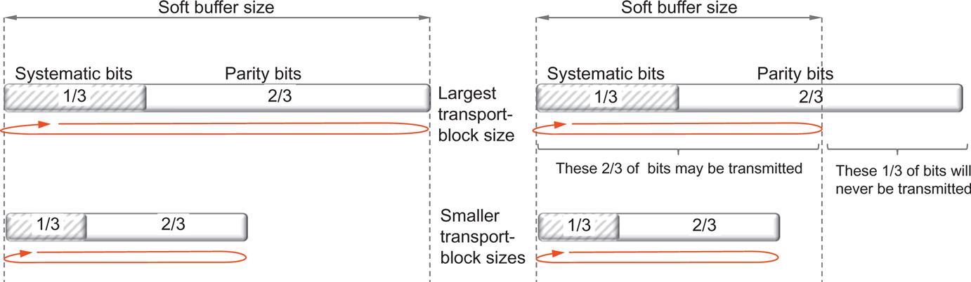
For the downlink, the device is not required to buffer more soft bits than corresponding to the largest transport block size coded at rate 2/3. Note that this only limits the soft buffer capacity for the highest transport block sizes, that is, the highest data rates. For smaller transport block sizes, the device is capable of buffering all soft bits down to the mother code rate.

For the uplink, full-buffer rate matching, where all soft bits are buffered irrespective of the transport block size, is supported given sufficient gNB memory. Limited-buffer rate matching using the same principles as for the downlink can be configured using RRC signaling.

The final step of the rate-matching functionality is to interleave the bits using a block interleaver and to collect the bits from each code block. The bits from the circular buffer are written row-by-row into a block interleaver and read out column-by-column. The number of rows in the interleaver is given by the modulation order and hence the bits in one column correspond to one modulation symbol³ (see Fig. 9.7). This results in the systematic bits spread across the modulation symbols, which improves performance. Bit collection concatenates the bits for each code block.

9.4 Scrambling

Scrambling is applied to the block of coded bits delivered by the hybrid-ARQ functionality by multiplying the sequence of coded bits with a bit-level scrambling sequence. Without scrambling, the channel decoder at the receiver could, at least in principle, be equally matched to an interfering signal as to the target signal, thus being unable to properly suppress the interference. By applying different scrambling sequences for neighboring cells in the downlink or for different devices in the uplink, the interfering signal(s) after descrambling is (are) randomized, ensuring full utilization of the processing gain provided by the channel code.

The scrambling sequence in both downlink (PDSCH) and uplink (PUSCH) depends on the identity of the device, that is, the C-RNTI, and a data scrambling identity configured in each device. If no data scrambling identity is configured, the physical layer cell identity is used as a default value to ensure that neighboring devices, both in the same cell and between cells, use different scrambling sequences. Furthermore, in the case of two transport blocks being transmitted in the downlink to support more than four layers, different scrambling sequences are used for the two transport blocks.

9.5 Modulation

The modulation step transforms the block of scrambled bits to a corresponding block of complex modulation symbols. The modulation schemes supported include QPSK, 16QAM, 64QAM, and 256QAM in both uplink and downlink. In addition, for the uplink π/2-BPSK is supported in the case the DFT-precoding is used, motivated by a reduced cubic metric [60] and hence improved power-amplifier efficiency, in particular for coverage limited scenarios. Note that π/2-BPSK is neither supported nor useful in the absence of DFT-precoding as the cubic metric in this case is dominated by the OFDM waveform.

9.6 Layer Mapping

The purpose of the layer-mapping step is to distribute the modulation symbols across the different transmission layers. This is done in a similar way as for LTE; every nth symbol is mapped to the nth layer. One coded transport block can be mapped on up to four layers. In the case of five to eight layers, supported in the downlink only, a second transport block is mapped to layers five to eight following the same principle as for the first transport block.

Multi-layer transmission is only supported in combination with OFDM, the baseline waveform in NR. With DFT-precoding in the uplink, only a single transmission layer is supported. This is motivated both by the receiver complexity, which in the case of multi-layer transmission would be significantly higher with a DFT-precoder than without, and the use case originally motivating the additional support of DFT-precoding, namely handling of coverage-limited scenarios. In such a scenario, the received signal-to-noise ratio is too low for efficient usage of spatial multiplexing and there is no need to support spatial multiplexing to a single device.

9.7 Uplink DFT Precoding

DFT precoding can be configured in the uplink only. In the downlink, as well as the case of OFDM in the uplink, the step is transparent.

In the case that DFT-precoding is applied in the uplink, blocks of M symbols are fed through a size-M DFT as illustrated in Fig. 9.8, where M corresponds to the number of subcarriers assigned for the transmission. The reason for the DFT precoding is to reduce the cubic metric for the transmitted signal, thereby enabling higher power-amplifier efficiency. From an implementation complexity point of view the DFT size should preferably be constrained to a power of 2. However, such a constraint would limit the scheduler flexibility in terms of the amount of resources that can be assigned for an uplink transmission. Rather, from a flexibility point of view all possible DFT sizes should preferably be allowed. For NR, the same middle-way as for LTE has been adopted where the DFT size, and thus also the size of the resource allocation, is limited to products of the integers 2, 3, and 5. Thus, for example, DFT sizes of 60, 72, and 96 are allowed but a DFT size of 84 is not allowed.⁴ In this way, the DFT can be implemented as a combination of relatively low-complex radix-2, radix-3, and radix-5 FFT processing.

9.8 Multi-Antenna Precoding

The purpose of multi-antenna precoding is to map the different transmission layers to a set of antenna ports using a precoder matrix. In NR, the precoding and multi-antenna operation differs between downlink and uplink and the codebook-based precoding step is, except for CSI reporting, only visible in the uplink direction. For a detailed discussion on how the precoding step is used to realize beamforming and different multi-antenna schemes see Chapters 11 and 12.

9.8.1 Downlink Precoding

In the downlink, the demodulation reference signal (DMRS) used for channel estimation is subject to the same precoding as the PDSCH (see Fig. 9.9). Thus, the precoding is not explicitly visible to the receiver but is seen as part of the overall channel. This is similar to the receiver-transparent spatial filtering discussed in the context of CSI-RS and SRS in Chapter 8. In essence, in terms of actual downlink transmission, any multi-antenna precoding can be seen as part of such, to the device, transparent spatial filtering.

However, for the purpose of CSI reporting, the device may assume that a specific precoding matrix W is applied at the network side. The device is then assuming that the precoder maps the signal to the antenna ports of the CSI-RS used for the measurements on which the reporting was done. The network is still free to use whatever precoder it finds advantageous for data transmission.

To handle receiver-side beamforming, or in general multiple reception antennas with different spatial characteristics, QCL relations between a DM-RS port group, which is the antenna ports used for PDSCH transmission,⁵ and the antenna ports used for CSI-RS or SS block transmission can be configured. The Transmission Configuration Index (TCI) provided as part of the scheduling assignment indicates the QCL relations to use, or in other words, which reception beam to use. This is described in more detail in Chapter 12.

Demodulation reference signals are, as discussed in Section 9.11, transmitted in the scheduled resource blocks and it is from those reference signals that the device can estimate the channel, including any precoding W and spatial filtering F applied for PDSCH. In principle, knowledge about the correlation between reference signal transmissions, both in terms of correlation introduced by the radio channel itself and correlation in the use of precoder, is useful to know and can be exploited by the device to improve the channel estimation accuracy.

In the time domain, the device is not allowed to make any assumptions on the reference signals being correlated between PDSCH scheduling occasions. This is necessary to allow full flexibility in terms of beamforming and spatial processing as part of the scheduling process.

In the frequency domain, the device can be given some guidance on the correlation. This is expressed in the form of physical resource-block groups (PRGs). Over the frequency span of one PRG, the device may assume the downlink precoder remains the same and may exploit this in the channel-estimation process, while the device may not make any assumptions in this respect between PRGs. From this it can be concluded that there is a trade-off between the precoding flexibility and the channel-estimation performance—a large PRG size can improve the channel-estimation accuracy at the cost of precoding flexibility and vice versa. Hence, the gNB may indicate the PRG size to the device where the possible PRG sizes are two resource blocks, four resource blocks, or the scheduled bandwidth as shown in the bottom of Fig. 9.10. A single value may be configured, in which case this value is used for the PDSCH transmissions. It is also possible to dynamically, through the DCI, indicate the PRG size used. In addition, the device can be configured to assume that the PRG size equals the scheduled bandwidth in the case that the scheduled bandwidth is larger than half the bandwidth part.

9.8.2 Uplink Precoding

Similar to the downlink, uplink demodulation reference signals used for channel estimation are subject to the same precoding as the uplink PUSCH. Thus, also for the uplink the precoding is not directly visible from a receiver perspective but is seen as part of the overall channel (see Fig. 9.11).

However, from a scheduling point of view, the multi-antenna precoding of Fig. 9.1 is visible in the uplink as the network may provide the device with a specific precoder matrix W the receiver should use for the PUSCH transmission. This is done through the precoding information and antenna port fields in the DCI. The precoder is then assumed to map the different layers to the antenna ports of a configured SRS indicated by the network. In practice this will be the same SRS as the network used for the measurement on which the precoder selection was made. This is known as codebook-based precoding since the precoder W to use is selected from a codebook of possible matrices and explicitly signaled. Note that the spatial filter F selected by the device also can be seen as a precoding operation, although not explicitly controlled by the network. The network can however restrict the freedom in the choice of F through the SRS resource indicator (SRI) provided as part of the DCI.

There is also a possibility for the network to operate with non-codebook-based precoding. In this case W is equal to the identity matrix and precoding is handled solely by the spatial filter F based on recommendations from the device.

Both codebook-based and non-codebook-based precoding are described in detail in Chapter 11.

9.9 Resource Mapping

The resource-block mapping takes the modulation symbols to be transmitted on each antenna port and maps them to the set of available resource elements in the set of resource blocks assigned by the MAC scheduler for the transmission. As described in Section 7.3, a resource block is 12 subcarriers wide and typically multiple OFDM symbols, and resource blocks, are used for the transmission. The set of time–frequency resources used for transmission is determined by the scheduler. However, some or all of the resource elements within the scheduled resource blocks may not be available for the transport-channel transmission as they are used for:

The time–frequency resources to be used for transmission are signaled by the scheduler as a set of virtual resource blocks and a set of OFDM symbols. To these scheduled resources, the modulation symbols are mapped to resource elements in a frequency-first, time-second manner. The frequency-first, time-second mapping is chosen to achieve low latency and allows both the transmitter and receiver to process the data “on the fly”. For high data rates, there are multiple code blocks in each OFDM symbol and the device can decode those received in one symbol while receiving the next OFDM symbol. Similarly, assembling an OFDM symbol can take place while transmitting the previous symbols, thereby enabling a pipelined implementation. This would not be possible in the case of a time-first mapping as the complete slot needs to be prepared before the transmission can start.

The virtual resource blocks containing the modulation symbols are mapped to physical resource blocks in the bandwidth part used for transmission. Depending on the bandwidth part used for transmission, the carrier resource blocks can be determined and the exact frequency location on the carrier determined (see Fig. 9.12 for an illustration). The reason for this, at first sight somewhat complicated mapping process with both virtual and physical resource blocks is to be able to handle a wide range of scenarios.

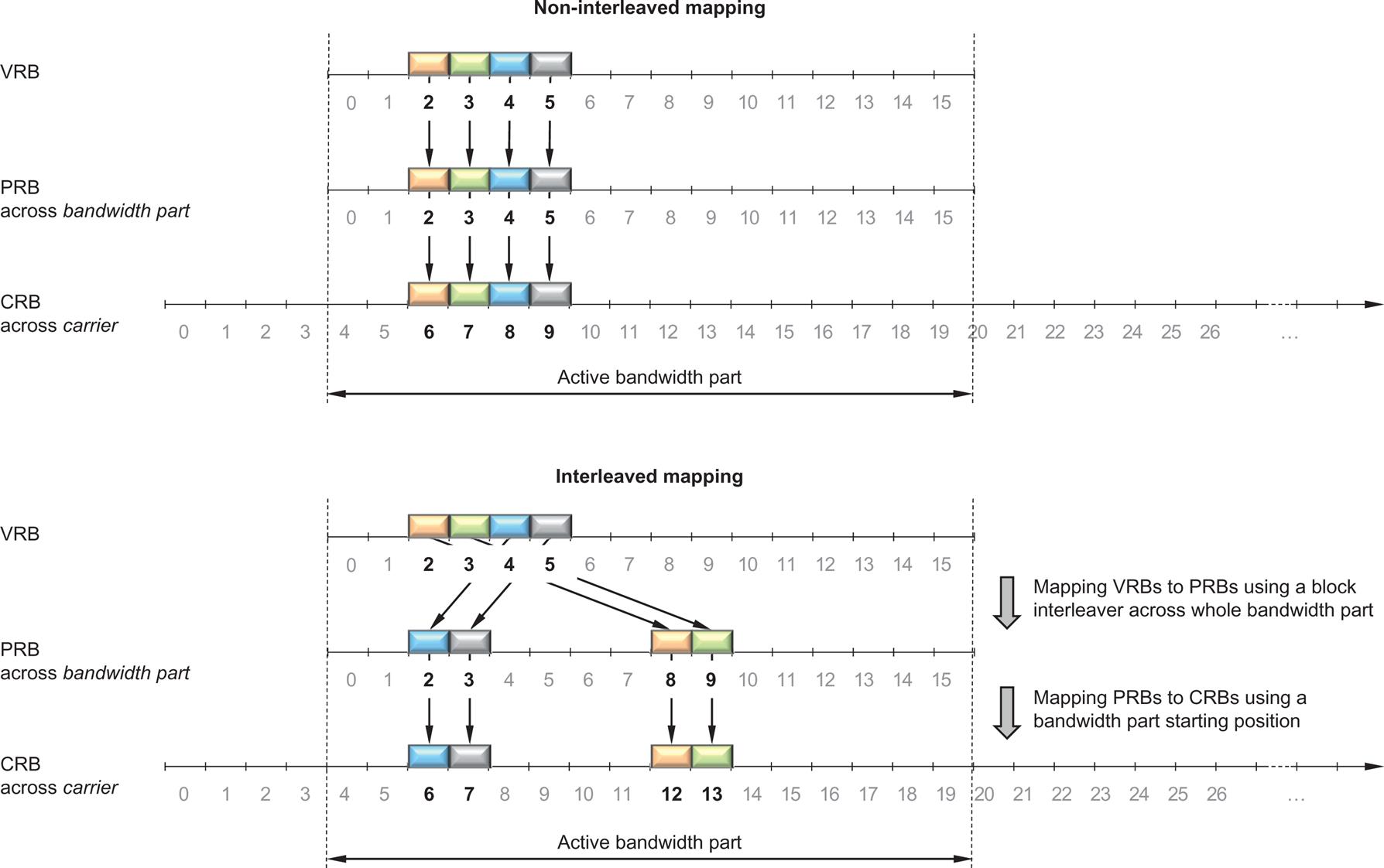
There are two methods for mapping virtual resource blocks to physical resource blocks, non-interleaved mapping (Fig. 9.12: top) and interleaved mapping (Fig. 9.12: bottom). The mapping scheme to use can be controlled on a dynamic basis using a bit in the DCI scheduling the transmission.

Non-interleaved mapping means that a virtual resource block in a bandwidth part maps directly to the physical resource block in the same bandwidth part. This is useful in cases when the network tries to allocate transmissions to physical resource with instantaneously favorable channel conditions. For example, the scheduler might have determined that physical resource blocks six to nine in Fig. 9.12 have favorable radio channel properties and are therefore preferred for transmission and a non-interleaved mapping is used.

Interleaved mapping maps virtual resource blocks to physical resource blocks using an interleaver spanning the whole bandwidth part and operating on pairs or quadruplets of resource blocks. A block interleaver with two rows is used, with pairs/quadruplets of resource blocks written column-by-column and read out row-by-row. Whether to use pairs or quadruplets of resource blocks in the interleaving operation is configurable by higher-layer signaling.

The reason for interleaved resource-block mapping is to achieve frequency diversity, the benefits of which can be motivated separately for small and large resource allocations.

For small allocations, for example voice services, channel-dependent scheduling may not be motivated from an overhead perspective due to the amount of feedback signaling required, or may not be possible due to channel variations not being possible to track for a rapidly moving device. Frequency diversity by distributing the transmission in the frequency domain is in such cases an alternative way to exploit channel variations. Although frequency diversity could be obtained by using resource allocation type 0 (see Section 10.1.10), this resource allocation scheme implies a relatively large control signaling overhead compared to the data payload transmitted as well as limited possibilities to signal very small allocations. Instead, by using the more compact resource allocation type 1, which is only capable of signaling contiguous resource allocations, combined with an interleaved virtual to physical resource block mapping, frequency diversity can be achieved with a small relative overhead. This is very similar to the distributed resource mapping in LTE. Since resource allocation type 0 can provide a high degree of flexibility in the resource allocation, interleaved mapping is supported for resource allocation type 1 only.

For larger allocations, possibly spanning the whole bandwidth part, frequency diversity can still be advantageous. In the case of a large transport block, that is, at very high data rates, the coded data are split into multiple code blocks as discussed in Section 9.2.2. Mapping the coded data directly to physical resource blocks in a frequency-first manner (remember, frequency-first mapping is beneficial from an overall latency perspective) would result in each code block occupying only a fairly small number of contiguous physical resource blocks. Hence, if the channel quality varies across the frequency range used for transmission, some code blocks may suffer worse quality than other code blocks, possibly resulting in the overall transport block failing to decode despite almost all code blocks being correctly decoded. The quality variations across the frequency range may occur even if the radio channel is flat due to imperfections in RF components. If an interleaved resource-block mapping is used, one code block occupying a contiguous set of virtual resource blocks would be distributed in the frequency domain across multiple, widely separated physical resource blocks, similarly to what is the case for the small allocations discussed in the previous paragraph. The result of the interleaved VRB-to-PRB mapping is a quality-averaging effect across the code blocks, resulting in a higher likelihood of correctly decoding very large transport blocks. This aspect of resource block mapping was not present in LTE, partially because the data rates were not as high as in NR, partly because the code blocks in LTE are interleaved.

The discussion above holds in general and for the downlink. In the uplink, release 15 only specifies RF requirements for contiguous allocations and therefore interleaved mapping is only supported for downlink transmissions. To obtain frequency diversity also in the uplink, frequency hopping can be used where the data in the first set of OFDM symbols in the slot are transmitted on the resource block as indicated by the scheduling grant. In the remaining OFDM symbols, data are transmitted on a different set of resource blocks given by a configurable offset from the first set. Uplink frequency hopping can be dynamically controlled using a bit in the DCI scheduling the transmission.

9.10 Downlink Reserved Resources

One of the key requirements on NR was to ensure forward compatibility, that is, to allow future extensions and technologies to be introduced in a simple way without causing backward-compatibility problems with, at that point in time, already-deployed NR networks. Several NR technology components contribute to meeting this requirement, but the possibility to define reserved resources in the downlink is one of the more important tools. Reserved resources are semistatically configured time–frequency resources around which the PDSCH can be rate-matched.

Reserved resources can be configured in three different ways:

There are no reserved resources in the uplink; avoiding transmission on certain resources can be achieved through scheduling.⁶

Configuring reserved resources by referring to a configured CORESET is used to dynamically control whether control signaling resources can be reused for data or not (see Section 10.1.2). In this case the reserved resource is identical to the CORESET configured and the gNB may dynamically indicate whether these resources are usable for PDSCH or not. Thus, reserved resources do not have to be periodically occurring but can be used when needed.

The third way to configure reserved resources is based on bitmaps. The basic building block for a resource-set configuration covers one or two slots in the time domain and can be described by two bitmaps as illustrated in Fig. 9.13:

If the resource set is defined on a carrier level, bitmap-1 has a length corresponding to the number of resource blocks within the carrier. If the resource set is bandwidth-part specific, the length of bitmap-1 is given by the bandwidth of the bandwidth part.

The same bitmap-1 is valid for all OFDM symbols indicated by bitmap-2. In other words, the same set of resource elements are reserved in all OFDM symbols indicated by bitmap-2. Furthermore, the frequency-domain granularity of the resource-set configuration provided by bitmap-1 is one resource block. In other words, all resource elements within a (frequency-domain) resource block are either reserved or not reserved.

Whether or not the resources configured as reserved resources are actually reserved or can be used for PDSCH can either be semistatically or dynamically controlled.

In the case of semistatic control, a third bitmap (bitmap-3) determines whether or not the resource-set defined by the bitmap-1/bitmap-2 pair or the CORSET is valid for a certain slot or not. The bitmap-3 has a granularity equal to the length of bitmap-2 (either one or two slots) and a length of 40 slots. In other words, the overall time-domain periodicity of a semistatic resource set defined by the triplet {bitmap-1, bitmap-2, bitmap-3} is 40 slots in length.

In the case of dynamic activation/deactivation of a rate-matching resource set, an indicator in the scheduling assignment indicates if the semistatically configured pattern is valid or not for a certain dynamically scheduled transmission. Note that, although Fig. 9.14 assumes scheduling on a slot basis, dynamic indication is equally applicable to transmission durations shorter than a slot. The indicator in the DCI should not be seen as corresponding to a certain slot. Rather, it should be seen as corresponding to a certain scheduling assignment. What the indicator does is simply indicate if, for a given scheduling assignment defined by a given DCI, a configured resource set should be assumed active or not during the time over which the assignment is valid.

In the general case, a device can be configured with up to eight different resource sets. Each resource set is configured either by referring to a CORSEST or by using the bitmap approach described above. By configuring more than one resource-set configuration, more elaborate patterns of reserved resources can be realized, as illustrated in Fig. 9.15.

Although a device can be configured with up to eight different resource-set configurations, each of which can be configured for dynamic activation, the configurations cannot be independently activated in the scheduling assignment. Rather, to maintain a reasonable overhead, the scheduling assignment includes at most two indicators. Each resource set configured for dynamic activation/deactivation is assigned to either one or both of these indications and jointly activates/deactivates or disables all resource sets assigned to that indicator. Fig. 9.15 illustrates an example with three configured resource sets, where resource set #1 and resource set #2 are assigned to indicator #1 and indicator #2, respectively, while resource set #2 is assigned to both indicators. Note that the patterns in Fig. 9.15 are not necessarily realistic, but rather chosen for illustrative purposes.

9.11 Reference Signals

Reference signals are predefined signals occupying specific resource elements within the downlink time–frequency grid. The NR specification includes several types of reference signals transmitted in different ways and intended to be used for different purposes by a receiving device.

Unlike LTE, which relies heavily on always-on, cell-specific reference signals in the downlink for coherent demodulation, channel quality estimation for CSI reporting, and general time–frequency tracking, NR uses different downlink reference signals for different purposes. This allows for optimizing each of the reference signals for their specific purpose. It is also in line with the overall principle of ultralean transmission as the different reference signals can be transmitted only when needed. Later release of LTE took some steps in this direction, but NR can exploit this to a much larger degree as there are no legacy NR devices to cater for.

The NR reference signals include:

In the following, the demodulation reference signals intended for coherent demodulation of PDSCH and PUSCH are described in more detail, starting with the reference signal structure used for OFDM. The same DM-RS structure is used for both downlink and uplink in the case of OFDM. For DFT-spread OFDM in the uplink, a reference signal based on Zadoff–Chu sequences as in LTE is used to improve the power-amplifier efficiency but supporting contiguous allocations and single-layer transmission only as discussed in a later section. Finally, a discussion on the phase-tracking reference signal is provided.

9.11.1 Demodulation Reference Signals for OFDM-Based Downlink and Uplink

The DM-RS in NR provides quite some flexibility to cater for different deployment scenarios and use cases: a front-loaded design to enable low latency, support for up to 12 orthogonal antenna ports for MIMO, transmissions durations from 2 to 14 symbols, and up to four reference-signal instances per slot to support very high-speed scenarios.

To achieve low latency, it is beneficial to locate the demodulation reference signals early in the transmission, sometimes known as front-loaded reference signals. This allows the receiver to obtain a channel estimate early and, once the channel estimate is obtained, process the received symbols on the fly without having to buffer a complete slot prior to data processing. This is essentially the same motivation as for the frequency-first mapping of data to the resource elements.

Two main time-domain structures are supported, differencing in the location of the first DM-RS symbol:

• • Mapping type A, where the first DM-RS is located in symbol 2 or 3 of the slot and the DM-RS is mapped relative to the start of the slot boundary, regardless of where in the slot the actual data transmission starts. This mapping type is primarily intended for the case where the data occupy (most of) a slot. The reason for symbol 2 or 3 in the downlink is to locate the first DM-RS occasion after a CORESET located at the beginning of a slot.
• • Mapping type B, where the first DM-RS is located in the first symbol of the data allocation, that is, the DM-RS location is not given relative to the slot boundary but rather relative to where the data are located. This mapping is originally motivated by transmissions over a small fraction of the slot to support very low latency and other transmissions that benefit from not waiting until a slot boundary starts but can be used regardless of the transmission duration.

The mapping type for PDSCH transmission can be dynamically signaled as part of the DCI (see Section 9.11 for details), while for the PUSCH the mapping type is semistatically configured.

Although front-loaded reference signals are beneficial from a latency perspective, they may not be sufficiently dense in the time domain in the case of rapid channel variations. To support high-speed scenarios, it is possible to configure up to three additional DM-RS occasions in a slot. The channel estimator in the receiver can use these additional occasions for more accurate channel estimation, for example, to use interpolation between the occasions within a slot. It is not possible to interpolate between slots, or in general different transmission occasions, as different slots may be transmitted to different devices and/or in different beam directions. This is a difference compared to LTE, where interslot interpolation of the channel estimates is possible but also restricts the multi-antenna and beamforming flexibility in LTE compared to NR.

The different time-domain allocations for DM-RS are illustrated in Fig. 9.16, including both single-symbol and double-symbol DM-RS. The purpose of the double-symbol DM-RS is primarily to provide a larger number of antenna ports than what is possible with a single-symbol structure as discussed below. Note that the time-domain location of the DM-RS depends on the scheduled data duration. Furthermore, not all patterns illustrated in Fig. 9.16 are applicable to the PDSCH (for example, mapping type B for PDSCH only supports duration 2, 4, and 7.

Multiple orthogonal reference signals can be created in each DM-RS occasion. The different reference signals are separated in the frequency and code domains, and, in the case of a double-symbol DM-RS, additionally in the time domain. Two different types of demodulation reference signals can be configured, type 1 and type 2, differing in the mapping in the frequency domain and the maximum number of orthogonal reference signals. Type 1 can provide up to four orthogonal signals using a single-symbol DM-RS and up to eight orthogonal reference signals using a double-symbol DM-RS. The corresponding numbers for type 2 are six and twelve. The reference signal types (1 or 2) should not be confused with the mapping types (A or B); different mapping types can be combined with different reference signal types.

Reference signals should preferably have small power variations in the frequency domain to allow for a similar channel-estimation quality for all frequencies spanned by the reference signal. Note that this is equivalent to a well-focused time-domain autocorrelation of the transmitted reference signal. For OFDM-based modulation, a pseudo-random sequence is used, more specifically a length 2³¹–1 Gold sequence, which fulfills the requirements on a well-focused autocorrelation. The sequence is generated across all the common resource blocks (CRBs) in the frequency domain but transmitted only in the resource blocks used for data transmission as there is no reason for estimating the channel outside the frequency region used for transmission. Generating the reference signal sequence across all the resource blocks ensures that the same underlying sequence is used for multiple devices scheduled on overlapping time–frequency resources in the case of multi-user MIMO (see Fig. 9.17) (orthogonal sequences are used on top of the pseudo-random sequence to obtain multiple orthogonal reference signals from the same pseudo-random sequence as discussed later). If the underlying pseudo-random sequence would differ between different co-scheduled devices, the resulting reference signals would not be orthogonal. The pseudo-random sequence is generated using a configurable identity, similar to the virtual cell ID in LTE. If no identity has been configured, it defaults to the physical-layer cell identity.

Returning to the type 1 reference signals, the underlying pseudo-random sequence is mapped to every second subcarrier in the frequency domain in the OFDM symbol used for reference signal transmission, see Fig. 9.18 for an illustration assuming only front-loaded reference signals are being used. Antenna ports⁷ 1000 and 1001 use even-numbered subcarriers in the frequency domain and are separated from each other by multiplying the underlying pseudo-random sequence with different length-2 orthogonal sequences in the frequency domain, resulting in transmission of two orthogonal reference signals for the two antenna ports. As long as the radio channel is flat across four consecutive subcarriers, the two reference signals will be orthogonal also at the receiver. Antenna ports 1000 and 1001 are said to belong to CDM group 0 as they use the same subcarriers but are separated in the code-domain using different orthogonal sequences. Reference signals for antenna ports 1002 and 1003 belong to CDM group 1 and are generated in the same way using odd-numbered subcarriers, that is, separated in the code domain within the CDM group and in the frequency domain between CDM groups. If more than four orthogonal antenna ports are needed, two consecutive OFDM symbols are used instead. The structure above is used in each of the OFDM symbols and a length-2 orthogonal sequence is used to extend the code-domain separation to also include the time domain, resulting in up to eight orthogonal sequences in total.

Demodulation reference signals type 2 (see Fig. 9.19) have a similar structure to type 1, but there are some differences, most notably the number of antenna ports supported. Each CDM group for type 2 consists of two neighboring subcarriers over which a length-2 orthogonal sequence is used to separate the two antenna ports sharing the same set of subcarriers. Two such pairs of subcarriers are used in each resource block for one CDM group. Since there are 12 subcarriers in a resource block, up to three CDM groups with two orthogonal reference signals each can be created using one resource block in one OFDM symbol. By using a second OFDM symbol and a time-domain length-2 sequence in the same was as for type 1, a maximum of 12 orthogonal reference signals can be created with type 2. Although the basic structures of type 1 and type 2 have many similarities, there are also differences. Type 1 is denser in the frequency domain, while type 2 trades the frequency-domain density for a larger multiplexing capacity, that is, a larger number of orthogonal reference signals. This is motivated by the support for multi-user MIMO with simultaneous transmission to a relatively large number of devices.

The reference signal structure to use is determined based on a combination of dynamic scheduling and higher-layer configuration. If a double-symbol reference signal is configured, the scheduling decision, conveyed to the device using the downlink control information, indicates to the device whether to use single-symbol or double-symbol reference signals. The scheduling decision also contains information for the device which reference signals (more specifically, which CDM groups) that are intended for other devices (see Fig. 9.20). The scheduled device maps the data around both its own reference signals as well as the reference signals intended for another device. This allows for a dynamic change of the number of coscheduled devices in the case of multi-user MIMO. In the case of spatial multiplexing (also known as single-user MIMO) of multiple layers for the same device, the same approach is used—each layer leaves resource elements corresponding to another CDM group intended for the same device unused. This is to avoid interlayer interference for the reference signals.

The reference signal description above is applicable to both uplink and downlink. Note though, that for precoder-based uplink transmissions, the uplink reference signal is applied before the precoder (see Fig. 9.11). Hence, the reference signal transmitted is not the structure above, but the precoded version of it.⁸

9.11.2 Demodulation Reference Signals for DFT-Precoded OFDM Uplink

DFT-precoded OFDM supports single-layer transmission only and is primarily designed with coverage-challenged situations in mind. Due to the importance of low cubic metric and corresponding high power-amplifier efficiency for uplink DFT-precoded OFDM, the reference signal structure is somewhat different compared to the OFDM case. In essence, transmitting reference signals frequency multiplexed with other uplink transmissions from the same device is not suitable for the uplink as that would negatively impact the device power-amplifier efficiency due to increased cubic metric. Instead, certain OFDM symbols within a slot are used exclusively for DM-RS transmission—that is, the reference signals are time multiplexed with the data transmitted on the PUSCH from the same device. The structure of the reference signal itself then ensures a low cubic metric within these symbols as described below.

In the time domain, the reference signals follow the same mapping as configuration type 1. As DFT-precoded OFDM is capable of single-layer transmission only and DFT-precoded OFDM is primarily intended for coverage-challenged situations, there is no need to support configuration type 2 and its capability of handling a high degree of multi-user MIMO. Furthermore, since multi-user MIMO is not a targeted scenario for DFT-precoded OFDM, there is no need to define the reference signal sequence across all common resource blocks as for the corresponding OFDM case, but it is sufficient to define the sequence for the transmitted physical resource blocks only.

Uplink reference signals should preferably have small power variations in the frequency domain to allow for similar channel-estimation quality for all frequencies spanned by the reference signal. As already discussed, for OFDM transmission it is fulfilled by using a pseudo-random sequence with good autocorrelation properties. However, for the case of DFT-precoded OFDM, limited power variations as a function of time are also important to achieve a low cubic metric of the transmitted signal. Furthermore, a sufficient number of reference-signal sequences of a given length, corresponding to a certain reference-signal bandwidth, should be available in order to avoid restrictions when scheduling multiple devices in different cells. A type of sequence fulfilling these two requirements is the Zadoff–Chu sequence, discussed in Chapter 8. From a Zadoff–Chu sequence with a given group index and sequence index, additional reference-signal sequences can be generated by applying different linear phase rotations in the frequency domain, as illustrated in Fig. 9.21. This is the same principle as used in LTE.

9.11.3 Phase-Tracking Reference Signals (PT-RS)

Phase-tracking reference signals (PT-RS) can be seen as an extension to DM-RS, intended for tracking phase variations across the transmission duration, for example, one slot. These phase variations can come from phase noise in the oscillators, primarily at higher carrier frequencies where the phase noise tends to be higher. It is an example of a reference signal type existing in NR but with no corresponding signal in LTE. This is partially motivated by the lower carrier frequencies used in LTE, and hence less problematic phase noise situation, and partly it is motivated by the presence of cell-specific reference signals in LTE which can be used for tracking purposes. Since the main purpose is to track phase noise, the PT-RS needs to be dense in time but can be sparse in frequency. The PT-RS only occurs in combination with DM-RS and only if the network has configured the PT-RS to be present. Depending on whether OFDM or DFTS-OFDM is used, the structure differs.

For OFDM, the first reference symbol (prior to applying any orthogonal sequence) in the PDSCH/PUSCH allocation is repeated every Lth OFDM symbol, starting with the first OFDM symbol in the allocation. The repetition counter is reset at each DM-RS occasion as there is no need for PT-RS immediately after a DM-RS. The density in the time-domain is linked to the scheduled MCS in a configurable way.

In the frequency domain, phase-tracking reference signals are transmitted in every second or fourth resource block, resulting in a sparse frequency domain structure. The density in the frequency domain is linked to the scheduled transmission bandwidth such that the higher the bandwidth, the lower the PT-RS density in the frequency domain. For the smallest bandwidths, no PT-RS is transmitted.

To reduce the risk of collisions between phase-tracking reference signals associated with different devices scheduled on overlapping frequency-domain resources, the subcarrier number and the resource blocks used for PT-RS transmission are determined by the C-RNTI of the device. The antenna port used for PT-RS transmission is given by the lowest numbered antenna port in the DM-RS antenna port group. Some examples of PT-RS mappings are given in Fig. 9.22.

For DFT-precoded OFDM in the uplink, the samples representing the phase-tracking reference signal are inserted prior to DFT precoding. The time domain mapping follows the same principles as the pure OFDM case.