3
User-Created Functions, Repetitive Operations, and Conditionals
3.1 Introduction
In this chapter, we shall introduce several ways to create functions, exercise program control by using If and Which, and perform repetitive operations by using Do, While, Nest, and Map.
There are several reasons to create functions: avoid duplicate code; limit the effect of changes to specific sections of a program; reduce the apparent complexity of the overall program by making it more readable and manageable; isolate complex operations; and perhaps make debugging and error isolation easier.
3.2 Expressions and Procedures as Functions
3.2.1 Introduction
An expression is any legitimate combination of Mathematica objects such as a mathematical formula, a list, a graphical entity, or a built-in function. Mathematica evaluates each expression in any of several ways; for example, by computing the expression (1 + 2 → 3), by simplifying it (a − 4a + 2 → 2 − 3a), or by executing a definition (r = 7 → 7). During the evaluation process, an attempt is made by Mathematica to reduce expressions to a standard form.
A procedure is a sequence of expressions to be evaluated. When this procedure is used once, it can appear within one cell and be evaluated after all the expressions have been entered or it can be evaluated on an expression-by-expression basis. However, when a procedure will be used more than once or it will be used by a built-in function, it is better to create a special object called a function. There are several ways to create a function: all but one of these ways uses global variables; the one that can create local variables is Module. They are all implemented in a similar manner.
When one expression is to be made into a function, a common way to create it is with
examfcn[x_,y_,…]:=expr1
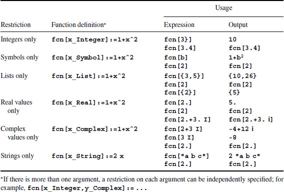
where examfcn is the function name created by the programmer, the underscore (_) is required for the arguments x_, y_, … , and expr1 is a function of x, y, … . The colon preceding the equal sign tells Mathematica that expr1 will be evaluated anew every time that examfcn is implemented (used). Lastly, each of the arguments x_, y_, … , can be a numerical value or a list of numerical values, a symbolic expression, or a function; either a built-in function or a user-defined function. In addition, as shown in Table 3.1, each input variable can be subject to a condition to ensure that it is a specific type of variable. If that condition is not met, the function is not executed.
Table 3.1 Restrictions that can be placed on a function’s input variables
When the function is composed of M expressions, then the function is created with
    examfcn[x_,y_,…]:=(a1=expr1;
        a2=expr2;
        …
        exprM)
where the parentheses and semicolons are required. However, there is no semicolon after exprM. The result from the evaluation of the last expression, exprM, is the value of the function. If a semicolon were placed there, then the execution of examfcn would have no output. In creating the function indicated, each semicolon is followed by Enter and depending on the application, either Enter or Shift and Enter simultaneously is used after the closing parenthesis “)”. It is assumed that the quantities a1, a2, … , appear in one or more of the expressions following their introduction. The output exprM can be a single value exprM, a list {a1,a2,}, or an array {{a1,a2,…},{…},…}. Lastly, the variables a1, a2, … , are global variables; that is, they are permanently available to all subsequent expressions that use these variable names outside this function definition.
It is also noted that functions created by the user can be treated like any other expression: if appropriate, it can be numerically or symbolically differentiated, integrated, maximized, and so on.
These function-creation capabilities are now illustrated with several examples.
3.2.2 Pure Function: Function[]
Another syntax that can be used to create a function is with what is called a pure function. It is formally created with Function. However, in much of the material in the Documentation Center it appears in terms of a shorthand syntax that is best introduced by example. Although the pure function has all the attributes discussed above, its implementation is a little different.
Consider the function f(x,y) = x2 + ay3/x, where a is a constant. Using the previous syntax, a function representing f is given by
f[x_,y_]:=x^2+a y^3/x
Thus, to determine its value at x = 2.0 and y = 3.0, we use
f[2.,3.]
and find that
4.+13.5 a
A pure function on the other hand can be represented either of two ways. The first way is with
Function[{x,y,…},expr]
where {x,y,…} is a list of the independent variables and expr is an expression that is a function of the independent variables. Then, using this notation to create f(x,y), we have
ff=Function[{x,y},x^2+a y^3/x]
Then, as before, to determine its value at x = 2.0 and y = 3.0, we use
ff[2.,3.]
and find again that
4.+13.5 a
The second way to represent this function as a pure function is to employ the following syntax
g=#1^2+a #2^3/#1 &
In this expression, #1 represents one variable, x in this case, and #2 represents a second variable, y in this case. If there were only one variable, then #1 can be replaced with #. The expression is completed by ending it with a space after the last character followed by the &. In both cases, a is a global variable. In addition, g is shorthand for g[var1,var2] and although it cannot be explicitly written as such when created, it is employed in that way, as shown below.
The execution of the expression for g gives
![]() &
&
Then, to evaluate it, we use
g[2.,3.]
which yields the same as before; namely, 4.+13.5 a.
Again the evaluation of the pure function could be delayed in the same manner as the regular function by using the “:=” syntax; that is, g could have been written as
g:=#1^2+a #2^3/#1 &
Another way to employ the pure function is to provide the values for #1 and #2 immediately following the creation of the pure function as follows
g=#1^2+a #2^3/#1 &[2.,3.]
The execution of this expression displays the result previously obtained with g[2.,3.].
The use of a pure function also has utility in such operations as incrementing subscripts of symbolic variables and in placing units on numerical values. We shall illustrate this with several examples, each of which uses a pure function and Prefix, whose shorthand notation is /@ (recall Table 1.2).
To create a list of the integers 1 to 5 and their units, say acceleration, we use Quantity as follows
Quantity[#,"Meters"/"Seconds"^2] &/@Range[5]
which yields
{1 m/s2,2 m/s2,3 m/s2,4 m/s2,5 m/s2}
As a second example, a list of a symbolic variable that is subscripted from 1 to 5 will be created. The statement to do this operation is, with the use of the Basic Math Assistant,
a# &/@Range[5]
which results in
{a1,a2,a3,a4,a5}
As a third example, we shall create a 3×3 symbolic array containing the appropriate subscripts for each element. This task is most easily performed with the use of Array, which generates an (n×m) array of fnm elements. Its syntax is
Array[f,{n,m}]
where, in general, f is a function of n and m. Then the program is
Array[aToString[#1]<>ToString[#2]] &,{3,3}]//MatrixForm
which displays
For the last example, we shall create a 4×4 array whose elements are mn and display the result in matrix form. The value of m corresponds to the row position and n to the column position. The statement to perform these operations is
Array[#1^#2 &,{4,4}]//MatrixForm
which gives

3.2.3 Module[]
A third way that one can create a function is to use Module, which allows one to create local variables. The general form for Module is
heqn[xx_,yy_,…]:=Module[
    {x=xx,y=yy,…,a1,a2,…,b1=val1,b2=val2,…},proced]
where x, y, a1, a1, … , b1, b2, … , are local variables and proced is a procedure that is a function of the local variables and possibly other variables not placed between the preceding pair of braces {…}; these other variables will be global variables. The syntax b1=val1, b1=val1, … , additionally assigns the value (or a symbolic expression) given by val1 to b1, the value of val2 to b2, … . In addition, the form of the procedure follows the rules given previously for examfcn that contained M expressions; that is, a semicolon is placed at the end of each expression except the last one. It is mentioned again that, in general, exprM can be a list or an array.
We now illustrate the use of Module with the following example.
3.3 Find Elements of a List that Meet a Criterion: Select[]
Pure functions are frequently needed in certain Mathematica functions. One such function that uses pure functions is Select, which provides the means to select only those elements of a list that meet certain criteria. The definition of Select is
Select[list,crit]
where list is a vector list and crit is the criterion by which the elements of list will be evaluated. The argument crit is typically a pure function that operates on each element of list. Examples of some selection criteria are shown in Table 3.2. The output of Select is a list of the elements that satisfy the criteria in the precedence that they appear in the list.
Table 3.2 Examples of the use of Select[d,crit]

In addition, EvenQ, OddQ, Positive, and Negative given in Table 3.2 can be used individually as commands to determine the specific properties of the elements of a list. IntegerQ can be used on a single term only. EvenQ and OddQ are limited to integers only. The output of these commands is either True or False.
To illustrate their usage, consider the following example
d={6,-6,7,-7};
 Print["Even? ",EvenQ[d]]
 Print["Odd? ",OddQ[d]]
 Print["Positive? ",Positive[d]]
 Print["Negative? ",Negative[d]]
the output of which is
 Even? {True,True,False,False}
 Odd? {False,False,True,True}
 Positive? {True,False,True,False}
 Negative? {False,True,False,True}
3.4 Conditionals
In this section, we shall introduce several conditional functions and in Section 3.6 we shall give several examples of how they can be applied.
3.4.1 If[]
The test of a conditional or set of conditionals, denoted cond, is obtained with
r=If[cond,tr,fa] (* or If[cond,r=tr,r=fa] *)
where tr is selected if cond is true and r=tr, and fa is selected if cond is false and r=fa. In general, tr and fa can be a constant, an expression, or a procedure. When tr is a procedure, then each expression in the procedure is followed by a semicolon except the last expression. The last expression of tr is followed by a comma if fa is present, otherwise there is no punctuation.
3.4.2 Which[]
When a series of many conditionals cond1, cond2, … , condM have to be tested, one uses Which, whose form is
r=Which[cond1,tr1,cond2,tr2,…,condM,trM]
Here, each CondK, K = 1, 2, … , M is tested from left to right until a True is encountered at which point no more conditionals are tested. If True is encountered at K = L, then r=trL. In general, trK can be a constant, an expression, or a procedure. When trK is a procedure, then each expression in the procedure is followed by a semicolon except the last expression. The last expression is followed by a comma when K < M; when K = M, there is no punctuation.
3.5 Repetitive Operations
We shall introduce several functions that perform repetitive operations and in Section 3.6 we shall give several examples of how they can be applied.
3.5.1 Do[]
A specified number of repetitive operations are performed by Do. It is similar to Table, except that instead of forming a list it performs only an evaluation. The form for Do is
Do[expr,{n,ns,ne,dn}]
or
Do[expr,{n,{lst}}]
where expr is an expression or a procedure that is evaluated repetitively over the range of n and can be a function of the index n. The value of n is a quantity whose value starts at ns, ends at ne, and is incremented over this range by an amount dn or n can have the values of the elements appearing in {lst}. When expr is a procedure composed of M expressions expr1, expr2, … , exprM, then each expression is followed by a semicolon except exprM, which is followed by a comma.
3.5.2 While[]
The function While performs an indeterminate number of repetitive operations until a specified condition cond is met. The form for While is
While[cond,expr]
where expr is an expression or a procedure. When expr is a procedure composed of M expressions expr1, expr2, … , exprM, then each expression is followed by a semicolon except exprM, which has no punctuation.
3.5.3 Nest[]
The function Nest applies n times an operation f to an expression expr. Its form is
Nest[f,expr,n]
The operation f is typically expressed as a pure function.
A companion function called NestList performs in the same way that Nest does except that it presents in a list all the intermediate results; the first term in the list is expr and the last result is that given by Nest. A second related function is NestWhile, in which n in Nest is replaced by a test such that Nest continues until the test is satisfied. The test is typically expressed as a pure function. Nest can be used as a compact way to evaluate recurrence relations of the type yn+1 = g(yn).
3.5.4 Map[]
The function Map applies f to each element in an expression expr. Its form is
Map[f,expr] (* Alternate form: f/@expr *)
This function is best understood by illustrating its capabilities. For example, to create a table of the evaluation of several elementary functions of, say, the number 2 and label these functions, we use Map as follows
Map[{#[2],#[2.]} &,{Sin,Cos,Tan,Cot,Exp,Sqrt}]//Column
which displays

In using Map this way, we have taken advantage of how Mathematica treats integers and decimal quantities: with integers no numerical evaluation is performed and with decimal numbers it is.
For another example, we shall add the same pair of elements {x,y} to the square of each respective component of the list {{z1,z2},{z3,z4}, …}; that is, we shall create the list ![]() . Thus,
. Thus,
c={{1,2},{3,4},{5,6}};
 Map[#^2+{x,y} &,c]
gives
{{1+x,4+y},{9+x,16+y},{25+x,36+y}}
3.6 Examples of Repetitive Operations and Conditionals
3.7 Functions Introduced in Chapter 3
In addition to the functions listed in Tables 3.1 and 3.2, the additional functions introduced in this chapter are listed in Table 3.3.
Table 3.3 Summary of additional commands introduced in Chapter 3
| Command | Usage |
| Array | Generates lists and arrays of specified size and with specified elements |
| ArrayFlatten | Flattens arrays according to specified rules |
| Do | Perform a series of operations a specified number of times or using a set of specified values |
| EvenQ | Gives True if its argument is an even integer, False otherwise |
| If | Evaluates a conditional expression to determine whether it is true or false |
| Map | Applies a function to each element of a list |
| Module | Creates a function in which some or all of the variables can be local |
| Negative | Gives True if its argument is a negative number, False otherwise |
| Nest | Applies an operation to an expression a specified number of times |
| NestList | Give the intermediate results of Nest |
| NestWhile | Performs as Nest but continues until a specified condition is satisfied |
| OddQ | Gives True if its argument is an odd integer, False otherwise |
| Positive | Gives True if its argument is a positive number, False otherwise |
| Reap | See Example 3.15 |
| Select | Identifies all elements of a list that meet a specified criterion |
| Sow | See Example 3.15 |
| Which | An efficient way to test numerous conditional expressions |
| While | Repetitively evaluates a conditional expression until it is satisfied |
| With | A means to replace variables with other symbols or values |
Exercises
Section 3.2.2
- 3.1 The elements of an (N×N) matrix are given by
Use Array to generate these elements for N = 8 and display the results in matrix form.
Sections 3.4.1 and 3.5.1
- 3.2 Consider a function f(x) in the region a ≤ x ≤ b. Sample f(x) at xn, n = 1, 2, … , N, where xn − xn−1 = (b − a)/(N − 1) and x1 = a and xN = b. Then, for a given f(x), a, b, and N, create a program that determines the first M changes in the sign of f(x) in this region and the values xk and xk−1 that define each region in which this sign change takes place. Recall that a sign change occurs when the product f(xk)f(xk−1) is negative. Recall Example 3.8.
Verify your program by finding the values of xk and xk−1 for the first four sign changes (M = 4) of

for 1 ≤ Ω ≤ 25 and N = 41. The function J1(x) is the Bessel function of the first kind of order 1.
Section 3.5.1
- 3.3 Repeat Example 3.2 using nested Do commands.
Section 3.5.2
- 3.4 The complete elliptic integral K(α) can be computed as

where aN is determined in the following manner. We set a0 = 1, b0 = cosα and c0 = sinα and employ the recurrence relations

such that when |cN| < to, where to is a specified tolerance, we say that the process has converged to K(α). Setting to = 0.00001 and α = π/4, verify that this process converges to the correct value by comparing it to the value obtained from EllipticK[Sin[α]^2].
- 3.5 Consider the following series
where
Find the value of M for which

Section 3.5.3
- 3.6 The total interest paid iT on a loan L over M months at an annual interest rate ia is obtained from
where
The quantity pmon is the monthly payment of interest and principal, im = ia/1200, and b0 = L. Determine iT for ia = 6.5%, M = 240 months, and L = $150,000.