One part of solving engineering problems is to apply one or more solution methods until a form that is amenable to numerical procedures and computer evaluation is obtained. We shall illustrate in this chapter how one can use the symbolic capabilities of Mathematica to meet these goals. One advantage of using symbolic solutions is that once their symbolic solution is known it can be converted to a function and used to perform parametric studies or used in other applications.
We shall illustrate two types of symbolic manipulations. The first type is concerned with the simplification and manipulation of the symbolic expressions to attain a form more suitable for one’s end usage. The second type is to perform a mathematical operation on a symbolic expression such as finding its derivative, integrating it, and the like.
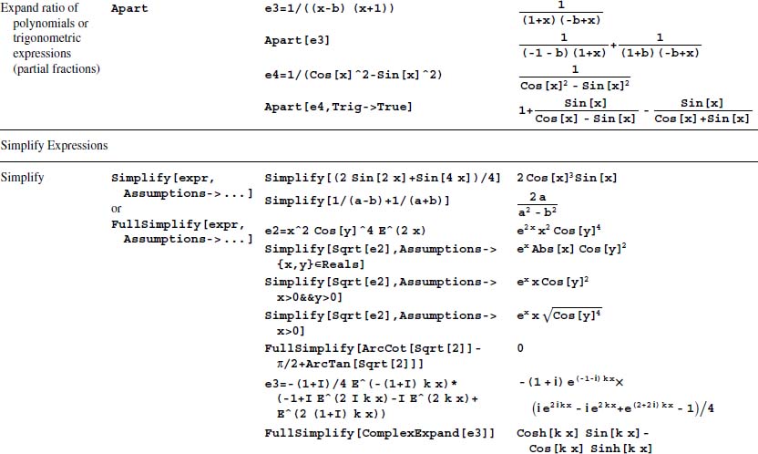
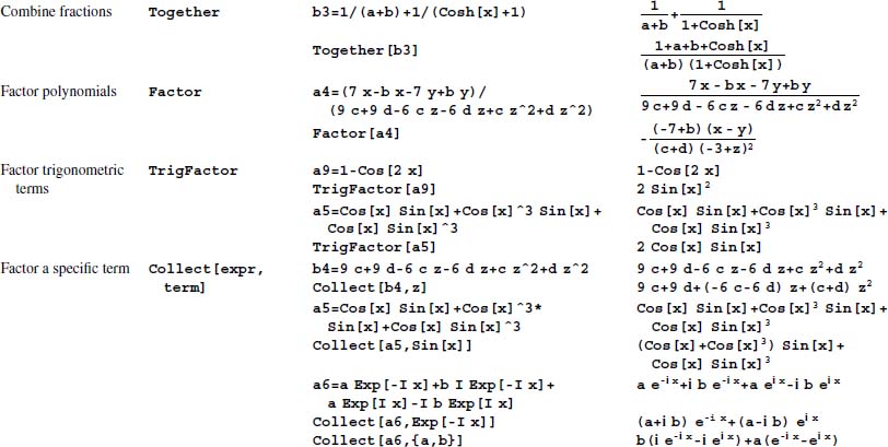
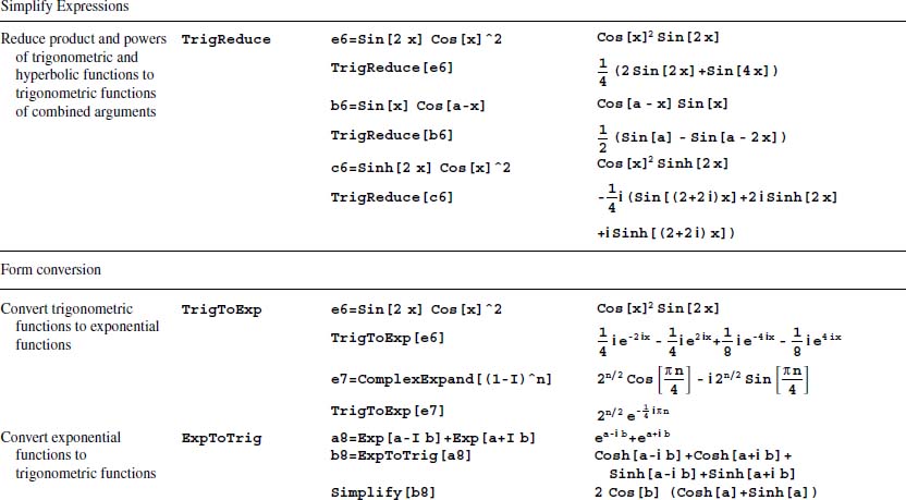
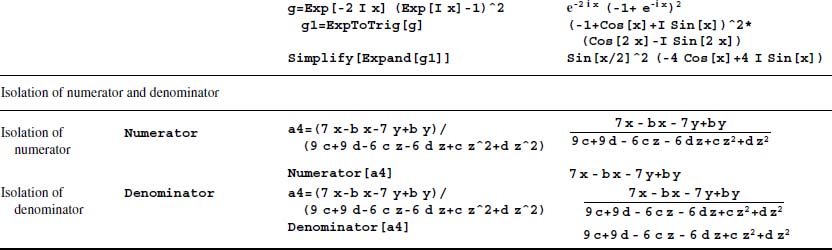
Several simplification and manipulation commands that are typically used on symbolic expressions are listed in Table 4.1. Also included in this table are illustrations of the usage of these functions.
The symbolic mathematical operations that will be illustrated are:
Solving equations—Solve[]
Limits—Limit[]
Power series—Series[] and Coefficient[]
Optimization—Maximize[]/Minimize[]
Differentiation—D[]
Integration—Integrate[]
Solutions to ordinary differential equations—DSolve[]
Solutions to some partial differential equations—DSolve[]
Laplace transform—LaplaceTransform[] and InverseLaplaceTransform[]
Not all differential equations and integrals have symbolic solutions; in these cases, one must obtain their solutions numerically. Therefore, in the next chapter, we shall re-visit some of these same operations using functions that employ numerical procedures to obtain their solutions.
For many uses of the symbolic operations, the most compact final forms of the results are often attained by operating on individual collections of terms and then placing each of them in their most compact form. Thus, the reader is encouraged to interact with the symbolic capabilities of Mathematica one line of code at a time. Several of the examples that follow employ this strategy.
4.2 Assumption Options
Many of the functions that we shall discuss in this chapter, including many of those appearing in Table 4.1, allow one to include assumptions concerning one or more of the symbols appearing in the expression being evaluated or manipulated. In those functions that accept Assumptions, the form can be either
…[…,Assumptions->{asum1, asum2,…}]
or
…[…,Assumptions->asum1 && asum2 && …]
where asumN are any of the assumptions appearing in the right-hand column of Table 4.2.
Table 4.2 Common assumptions that can be used in those Mathematica functions that accept them
Assumption*
Mathematica expression for assumption:+…,Assumptions->…&&… or
…,Assumptions->{…,…}
x is a real number
Element[x,Reals] or Reals
x is an integer
Element[x,Integers] or Integers
x is a complex number
Element[x,Complexes] or Complexes
x is a prime number
Element[x,Primes] or Primes
x > n or x ≥ n
x>n or x>=n
x<n or x ≤ n
x<n or x<=n
m<x<n or m ≤ x<n or m<x ≤ n or m ≤ x ≤ n
m<x<n or m<=x<n or m<x<=n or m<=x<=n
*x = variable name or a list of variable names that appear in the expression being operated on by the function; n, m = numerical or symbolic values.
+The symbol can be found in the Special Characters palette by selecting the Symbols tab, then the ≠ tab, and then going to the right-most column of the next to last row.
4.3 Solutions of Equations: Solve[]
The symbolic solutions to a set of equations, if they exist, are obtained by using either
sol=Solve[{eq1L==eq1R,eq2L==eq2R,…},vars]
or
sol=Solve[eq1L==eq1R && eq2L==eq2R &&…,vars]
where eqNR can be zero and vars is a list of the solution variables. The number of solution variables equals the number of equations.
4.4 Limits: Limit[]
The limit of an expression is obtained from
Limit[expr,x->xo,Assumptions->…]
where expr is a function of x and xo is a symbolic quantity or a numerical quantity, where -Infinity < xo < Infinity.
For example, to determine
we use
Limit[(1−Cos[x])/x,x->0]
and obtain 0.
4.5 Power Series: Series[], Coefficient[], and CoefficientList[]
One can obtain an nth-order power series approximation of an expression about the point x = xo with
Series[f,{x,xo,n}]
where f is the expression for which the series is to be obtained.
To illustrate the use of Series, we shall get a fourth-order series of the cosine of x about the point a. The statement to do this is
p=Series[Cos[x],{x,a,4}]
which gives
The expression O[x-a]5 represents a term on the order of (x − a)5. When a series is given in this form, one cannot use it for further numerical evaluation; that is, for example, p/.x−>2 results in an error message. To obtain an expression without this term and in a form that permits further numerical evaluation, the function Normal is used as follows
p=Normal[Series[Cos[x],{x,a,4}]]
Execution of this command results in the previous result, but without the last term O[x-a]5.
To be able to compare this result to those that follow, we shall expand p as follows
Expand[p]
which results in
The coefficients of the series can be accessed two ways. If expans is a polynomial in the powers of (x − a) up to the nth power, then the first way that the coefficients can be accessed is by using
Coefficient[expans,(x-a),m]]
which retrieves the coefficient associated with (x − a)m, n ≥ m ≥ 1, or with
CoefficientList[expans,x]
which gives a list of all the coefficients up to and including xn−1 (n ≥ 1).
For example, continuing with the expansion of cosine of x above,
Coefficient[p,(x-a),2]]
gives
whereas
Coefficient[p,x,2]]
gives
On the other hand,
CoefficientList[p,x]
displays
This list contains the coefficients of the expansion shown in Eq. (4.1), where the first element in the list contains the terms multiplying x0, the second element the terms multiplying x1, and so on.
4.6 Optimization: Maximize[]/Minimize[]
For a function f(x), the value of x = xm at which this function is a maximum/minimum and the magnitude of f(xm) is obtained from
Maximize[{f,con},x]Minimize[{f,con},x]
where f is the function to be maximized or minimized, con are any constraints that f is subject to, and x is the independent variable. The output of these functions is often fairly complex so that several other functions are frequently used in conjunction with them.
To isolate the expression corresponding to the value of f(xm), Maximize and Minimize, respectively, are replaced with
MaxValue[{f,con},x]MinValue[{f,con},x]
and to isolate the expression corresponding to xm, Maximize and Minimize, respectively, are replaced with
ArgMax[{f,con},x]ArgMin[{f,con},x]
One additional function that is used to further reduce the results to a specific region is
Refine[exp,assum]
where exp is a symbolic expression, in this case the output from one of the above functions, and assum are the assumptions that specify the region of interest.
The use of these functions is illustrated in the following example.
4.7 Differentiation: D[]
Differentiation with respect to one or more variables is performed using
D[f,{x1,n1},{x2,n2},…]
where f is an expression in one or more of the variables {x1,x2,…} and n1,n2,… are the orders of the derivatives in each variable. Thus, D also obtains the partial derivative. There are several equivalent syntaxes for D that, along with examples of their usage, are shown in Table 4.3. Also presented in this table are examples of D applied to several classes of functions.
Table 4.3 Examples of the symbolic derivative of different types of functions
For an example, consider the expression
To determine we proceed as follows
D[x^3 y^4,{x,2},{y,3}] (* or D[x^3 y^4,x,x,y,y,y] *)
which gives
144 x y
When f is a function of one variable, D can be replaced by a prime (′) provided that f is explicitly represented as a function of the independent variable. Consider the following expression
Then the second derivative of y can be determined using primes as follows
y[x_]=x^3 Cos[a x];y’’[x] (* or D[y[x],x,x] *)
The execution of these statements displays
6 x Cos[a x]-a2 x3 Cos[a x]−6 a x2 Sin[a x]
The command D can also be used to perform differentiation using functional representation and a change of variables. Consider the function f(u), where u = z(x). Then df/dx is obtained from
u=z[x];D[f[u],x] (* or in a compact form as D[f[z[x]],x] *)
which displays
f’[z[x]] z’[x]
where the prime denotes the derivative with respect to its argument; that is,
For example, if z = bxg, then we can use the previous command and the transformation rule to determine df/dx as follows
D[f[z[x]],x]/.D[z[x],x]->D[b x^g,x]
which gives
b g x−1+g f’[z[x]]
An expression for d2f/dx2 is obtained from
D[f[z[x]],x,x]
which displays
z’[x]^2 f’’[z[x]]+f’[z[x]] z’’[x]
where the prime denotes the derivative with respect to its argument; that is,
Again letting z = bxg, we can use the previous command and the transformation rule to determine d2f/dx2 as follows
where expr is, in general, a function of x, y, …, xlow is the lower x limit and xup is the upper x limit and similarly for the y variable ylow is the lower y limit and yup is the upper y limit. Either or both of the limits can be infinity; that is, Infinity (or ∞ from the appropriate template.)
When the integral cannot be found in terms of known functions, the system returns the Integrate statement as entered.
Before proceeding with several examples of the usage of Integrate, a command that has utility in evaluating integrals and in finding Laplace transforms, as well as other applications, is Piecewise, which is defined as
Piecewise[{{expr1,cond1},{expr2,cond2},…}]
where exprN are expressions and condN are most typically the ranges over which each exprN is to apply and is most often of the form aN ≤ x ≤ bN. An illustration of its usage is shown in Example 4.17.
Integration can also be performed using the appropriate template from the Advanced portion of the Calculator section of the Basic Math Assistant. Its usage is illustrated in Example 4.12.
4.9 Solutions of Ordinary Differential Equations: DSolve[]
The symbolic solutions to both ordinary and partial differential equations are obtained with
DSolve[{eqn1,eqn2,…},{y1,y2,…},{x1,x2,…}]
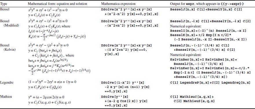
where {eqn1,eqn2,…} is a list of coupled differential equations and their boundary conditions, {y1,y2,…} is a list of the dependent variables appearing in {eqn1,eqn2,…}, and {x1,x2,…} is a list of the independent variables. When the system of equations is composed of ordinary differential equations, there is only one independent variable. When the boundary conditions are omitted, the system obtains a solution in terms of unknown constants C[n], where n goes from 1 to the order of the differential equation. In the list {eqn1,eqn2,…}, the representation of each dependent variable has to be given explicitly as y1[x1,x2,…], y2[x1,x1,…], …. Not all equations will have a symbolic solution. However, the solutions to many classical equations and some variations thereof are available and these solutions are presented in terms of special functions where appropriate. Several examples are shown in Table 4.4.
Table 4.4 Examples of the symbolic solution to well-known ordinary differential equations: n = 0, 1, 2, …
We shall illustrate the use of DSolve with the following examples. In several of these cases, the results will be plotted using the basic form of Plot, which is given in Table 6.1.
4.10 Solutions of Partial Differential Equations: DSolve[]
The symbolic solutions to a limited set of partial differential equations also can be obtained by using DSolve. We shall illustrate this capability with several examples. Before proceeding, it is noted that an important difference between the solutions obtained for ordinary differential equations and those obtained for partial differential equations is that the solution constants for ordinary differential equations are constants whereas those for partial differential equations may be functions of one or more of the independent variables.
4.11 Laplace Transform: LaplaceTransform[] and InverseLaplaceTransform[]
The Laplace transform is obtained from
LaplaceTransform[expr,t,s,Assumptions->{…}]
where s is the Laplace transform parameter, t is the independent variable that is being transformed, expr is an expression that is a function of t or is a constant, and Assumptions is used to place restrictions on any parameters appearing in expr. The initial conditions are dealt with by using Simplify and its Assumptions option.
Before proceeding, it is again noted that the definition of the unit step function u(x) as given by UnitStep[x] is used in Mathematica to represent a piecewise function such that u(x) = 0 for x< 0 and u(x) = 1 for x ≥ 0. Note that this definition includes 0. This is different from the Heaviside Theta function, which is given by HeavisideTheta. As mentioned in Example 4.20, this function is defined as 0 when its argument is < 0 and equal to 1 when its argument is > 0. It is not defined for an argument equal to 0.
We now consider the following example.
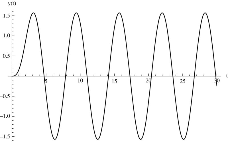
Figure 4.4 Graph of the numerical evaluation of the symbolic results of Example 4.29
Figure 4.5 Graph of the numerical evaluation of the inverse Laplace transform of Example 4.30. The curve with the larger magnitude is x2.
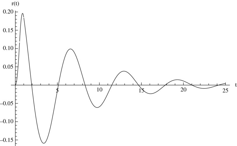
Figure 4.6 Graph of the numerical evaluation of the inverse Laplace transform of Example 4.31
4.12 Functions Introduced in Chapter 4
Listed in Table 4.5 are the functions introduced in this chapter that do not appear in Table 4.1.
Table 4.5 Summary of additional commands introduced in Chapter 4
Command
Usage
Coefficient
Gives the coefficient of a polynomial or power series
CoefficientList
Gives a list of the coefficients of a polynomial or a power series
D
Determines the ordinary or partial derivative or multiple derivative of a symbolic function
DiracDelta
Represents the delta function
Dsolve
Attempts to obtain a symbolic solution to an ordinary or partial differential equation
EulerEquations
Obtains the Euler–Lagrange equations [Requires loading of the Variational Methods Package]
HeavisideTheta
Represents the Heaviside theta function of argument x: when x< 0, output is 0; when x > 0, output is 1; undefined at x = 0
Integrate
Attempts to obtain a symbolic solution of an indefinite or definite integral
InverseLaplaceTransform
Attempts to determine the inverse Laplace transform
JordanDecomposition
Obtains [p] and [d] as the solution to [A] = [p][d][p]−1 for square matrices [A], [p], and [d] when [A] is given
LaplaceTransform
Attempts to determine the Laplace transform of an expression or an ordinary differential equation
Limit
Finds the limiting value of an expression
Normal
Converts some special forms of results to a normal form
Piecewise
Represents a piecewise function over the regions specified in its argument
Residue
Finds the residue of an expression at one of its singularities
Series
Gives the power series expansion of an expression or of a common function
Solve
Attempts to find a symbolic solution to an equation or system of equations
UnitStep
Represents the unit step function of argument x: when x< 0, output is 0; when x ≥ 0, output is 1
References
B. Balachandran and E. B. Magrab, Vibrations, 2nd edn, Cengage Learning, Toronto, Ontario, 2009, p. 472.
S. Timoshenko and S. Woinowsky-Krieger, Theory of Plates and Shells, 2nd edn, McGraw-Hill, New York, 1959, pp. 298–300.
Exercises
Table 4.1
4.1 The command TrigExpand and TrigReduce also work with hyperbolic functions. Consider the expression
Show that this can be reduced to
4.2 Find an expression for the real part of w in terms of trigonometric and hyperbolic functions when
Section 4.3
4.3 Solve for x when
4.4 Given the function
The value of x = xmax is that value at which the maximum value of f(x) occurs. It can be determined from the solution to df(x)/dx = 0 provided that d2f(xmax)/dx2< 0. Determine xmax.
4.5 Given the following system of equations
Determine expressions for ik.
4.6 Given the following set of equations
Solve for xj and then use the results in the following equation to obtain a cubic equation in h from which h can be determined
Do not solve for h.
4.7 If
then determine an expression for α, α > 0, that satisfies fm(α) = fm+1(α)
4.8 The nondimensional buckling load α of bar under a distributed axial load and resting on an elastic foundation can be determined from the determinant of the coefficients aj of
where γ is a nondimensional quantity that is proportional to the spring modulus of the elastic foundation.
Find the symbolic solution for α when K = 1 and when K = 3.
Find the numerical value of α when K = 1, 3, and 5 and γ = 0 and 0.4. Present the results in a table with the appropriate labels.
4.9 Given the following determinant
where Δ = Ω2 is a nondimensional frequency coefficient. Determine the smallest positive value of Ω when ka = π/4, ν = 0.3, and n = 0, 1, …, 10. Display the results in tabular form.
Section 4.4
4.10 Find the following limits
4.11 Find the limit of the following expression when n is an integer
Section 4.5
4.12 Obtain the coefficients of a five-term expansion of the following expression about = 0.
4.13 Obtain the coefficients of the polynomial in γ that result from expanding the determinant
4.14 Find the sum of the squares of the coefficients of the first five terms of the series expansion around x = 0
Section 4.7
4.15 Using the expression for the curvature of a parametric curve given in Example 4.10, show that when
the curvature is given by
Section 4.8
4.16 Evaluate the following integral when b > 0 and b is real.
4.17 Evaluate the following integral, which is proportional to the total radiation by a black body at all frequencies.
Section 4.9
4.18 The nondimensional transverse displacement y of a uniformly loaded annular circular plate with Poisson’s ratio ν is given by
Determine an expression for y when the boundary conditions at the inner boundary ξ = α, 0 <α< 1, are
and those at the outer boundary ξ = 1 are
Plot the results for y(ξ), y′(ξ), y′′(ξ), and y′′′(ξ) when α = 0.2 and ν = 0.3 using the grid plot commands of Example 4.20.
4.19 Determine the general solution to the following equation
where w = w(r), qo is a constant, and m = 0, 1, …, 5.
4.20 Consider a solid circular plate whose thickness varies as
where β is a constant. The governing equation for this type of plate when it is subjected to a nondimensional uniform load of magnitude p over the entire plate is given by [2, p. 298–300]
and w is the transverse displacement.
Verify that a particular solution to this equation is
Determine the solution to the homogeneous equation; that is, when p = 0.
If the solution is to remain finite at η = 0, then take the solution obtained in (b) and determine which part of the solution remains finite at η = 0.
4.21 In terms of nondimensional quantities, the governing equation of an annular circular plate whose thickness varies linearly and is subjected to a uniform load Qo distributed over the entire plate and a line load along the inner boundary of magnitude Po is given by [2, p. 303–305]
where ν is the Poisson’s ratio. Determine the solution to this equation when ν ≠ 1/3 and when ν = 1/3.
4.22 Given the following differential equation
where 1. Assume that an approximate solution to this equation is
Substitute this solution into the differential equation and generate a list of three equations of the form
Obtain a solution to these three, coupled equations.


 and n = 0, 1, …, 10. Display the results in tabular form.

 = 0.
= 0.


 1. Assume that an approximate solution to this equation is