6
Graphics
6.1 Introduction
There are many different ways to display numerical results and these different ways depend on whether the data are discrete, are obtained from expressions, require logarithmic compression, are to be represented in 2D or 3D, or are specific to a given application area such as statistics (histograms, bar charts, and pie charts), computational geometry (Voronoi diagrams and convex hulls), wavelet analysis, or controls (Bode, Nichols, and root locus plots). To accommodate these wide-ranging needs, Mathematica provides a large set of high-level plotting commands that require little user involvement to generate a basic figure; that is, one with minimum annotation. However, for each plot command, one is given the means to control virtually all aspects of the graph, thereby providing a high degree of flexibility in enhancing a figure. We shall discuss a subset of these plot commands and introduce instructions that can be used to modify, enhance, and individualize the graph’s curves and the overall figure.
Mathematica also provides a set of straightforward commands for creating an interactive environment for the presentation of numbers, expressions, and graphics by using Manipulate. This command is introduced in Chapter 7.
The introduction and usage of the various 2D and 3D plotting commands and their enhancement are introduced, primarily, via tables. The usage of these enhancements is then illustrated by examples from engineering topics.
6.2 2D Graphics
6.2.1 Basic Plotting
The basic forms of the 2D plotting commands that will be introduced in this chapter are presented in Table 6.1. They are divided into four categories: those that display the numerical evaluation of expressions using linear axes and those using logarithmic axes; and those that display lists of data using linear axes and those using logarithmic axes. It is mentioned that each plotting command that numerically evaluates an expression uses an internal procedure to determine the number and spacing of the values of the independent variable. These values are determined in a recursive fashion and the number of recursions that are used is, by default, determined automatically. However, if one wants to specify the number of recursions to n recursions, where n is a positive integer, this is done with the option MaxRecursion->n which is one of the optional arguments in the plotting command. Examples of the use of the 2D plot commands in Table 6.1 are shown in Tables 6.2 to 6.4.
Table 6.1 2D plotting commands for plotting one or more expressions or one or more lists of values. Optional enhancements, which are denoted enh, are comma-separated options given in subsequent tables
| Plotting type | Mathematica function* |
| Linear axes | |
| Basic | Plot[{f,g,…},{x,xs,xe},enh] |
| Parametric | ParametricPlot[{f,g},{x,xs,xe}},enh] |
| Polar | PolarPlot[r,{th,ths,the}},enh] |
| Contour | ContourPlot[h,{x,xs,xe},{y,ys,ye}},enh] |
| Region | RegionPlot[reg+,{x,xs,xe},{y,ys,ye}},enh] |
| Plotting expressions with logarithmic axes | |
| y-axis logarithmic, x-axis linear | LogPlot[{f,g,…},{x,xs,xe}},enh] |
| y-axis linear, x-axis logarithmic | LogLinearPlot[{f,g,…},{x,xs,xe}},enh] |
| y-axis logarithmic, x-axis logarithmic | LogLogPlot[{f,g,…},{x,xs,xe}},enh] |
| Plotting of lists of coordinate pairs with linear axes | |
| Basic: plot points only | ListPlot[{list1,list2,…} },enh] |
| Basic: connect data values | ListLinePlot[{list1,list2,…} },enh] |
| Polar | ListPolarPlot[{listr1,listr2,…} },enh] |
| Contour | ListContourPlot[lst,enh] |
| Plotting lists of coordinate pairs with logarithmic axes | |
| y-axis logarithmic, x-axis linear | ListLogPlot[{list1,list2,…} },enh] |
| y-axis linear, x-axis logarithmic | ListLogLinearPlot[{list1,list2,…} },enh] |
| y-axis logarithmic, x-axis logarithmic | ListLogLogPlot[{list1,list2,…} },enh] |
af = f(x), g = g(x); r = r(θ); h = h(x,y);
list1, list2, … , are lists of Cartesian coordinate pairs {{x1,y1},{x2,y2},…} ;
listr1 , listr2 , … , are lists of polar coordinate pairs {{th1,r1},{th2,r2},…} ;
xs or ys or ths = start value;
xe or ye or the = end value;
lst = {{x1,y1,f1},{x2,y2,f2},…}
b reg = is a set of relational equations each of which is separated by && ; reg is plotted only for those values of x and y that satisfy the set of relational equations.
Table 6.2 Examples of basic plotting expressions with linear axes
| Plot command | Expressions plotted and the plotting program | Figure created |
| Plot |  |
|
| ParametricPlot |  |
|
| PolarPlot | r(θ) = |J0(2π(0.6 − cos θ))|
r[ |
 |
| ContourPlot | w(x, y) = sin (2πx)sin (3πy)
w[x_,y_]:=Sin[2 |
 |
| RegionPlot | 13cos 2(x + y) ⩽ 92(x − 3)2 + 0.3(y − 1)2 ⩽ 3 RegionPlot[ 13 Cos[x+y]^2 <=9&& 2(x-3)^2+0.3 (y-1)^2 <=3, {x,1.3,4.5}, {y,-2.5,4.5}, AspectRatio->Automatic] |  |
Table 6.3 Examples of plotting expressions with logarithmic axes
| Plot command | Expressions plotted and the plotting program | Figure created |
| LogPlot | H(Ω) = {(1 − Ω2)2 + (0.1Ω)2}− 1/2 h[ |
 |
| LogLinearPlot | H(Ω) = {(1 − Ω2)2 + (0.1Ω)2}− 1/2
h[ |
 |
| LogLogPlot | H(Ω) = {(1 − Ω2)2 + (0.1Ω)2}− 1/2
h[ |
 |
Table 6.4 Examples of plotting of lists with linear axes. See also Table 6.15
| Plot command | Expressions used to generate discrete data and the plotting program | Figure created |
| ListPlot |  |
|
| ListLinePlot |  |
All figures can have their displayed size adjusted by employing the option
…[…, ImageSize->sz,…]
where typically sz is either Tiny, Small, Medium, or Large.
6.2.2 Basic Graph Enhancements
To enhance a figure, the arguments of the basic plotting commands given in Table 6.1 can be augmented with a very large set of optional instructions. We shall introduce several of them in this section and several others in the following sections.
Color
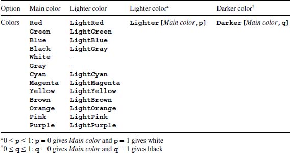
The named color attributes available for equations, text, curves, fill, regions, points, background, and graphics primitives are listed in Table 6.5. In addition to these named colors, each of the main colors can be made lighter by using Lighter or darker by using Darker as indicated in this table.
Table 6.5 Named color attributes available for equations, text, curves, fill, regions, graphics primitives, background, and points
There is also available a very large number of color schemes for use by such commands as ContourPlot, ListContourPlot, ParamentricPlot, RegionPlot, Plot3D, SphericalPlot3D, and the Filling option in Plot, ListPlot, and others. The color schemes are accessed with the Color Schemes palette obtained from the Palettes menu as shown in Figure 6.1 in either of two ways. The first way is to use

Figure 6.1 Selection of color schemes that are available from the Color Schemes palette
ColorFunction->ColorData["Color scheme name"]
where “Color scheme name” (quotation marks required) can be entered manually from any of the choices appearing in the palettes in any of the four headings: Gradient, Physical, Named, and Indexed. Shown in Figure 6.1 are the first few choices appearing under Gradient. The other choices become visible by scrolling down with the slider. The second way is to use the palette directly by typing the plotting option as
ColorFunction->
Leaving the cursor after the “>”, one goes to the palette menu and clicks on the desired selection and then clicks on Insert. When this is done for the palette selection shown in Figure 6.1, the following will appear
ColorFunction->ColorData["DarkRainbow"]
Curve Characteristics
Mathematica automatically selects the properties of the curves that it displays such that each curve is a different color, but each line is solid and has the same thickness. This automation can be overridden and line colors, line thickness, and the line type – solid or dashed – can be selected for each curve. The instruction to perform these changes is PlotStyle and illustrations of its usage are given in Table 6.6.
Table 6.6 Curve enhancements using PlotStyle
| PlotStyle->{{curve 1 attribute #1, curve 1 attribute #2,…},
{curve 2 attribute #1, curve 2 attribute #2,…},…}* |
|
| Option | curve k attribute #m |
| Dashed lines | Dashing[arg] arg = Tiny, Small, Medium, or Large ; arg = {} specifies a solid line |
| Line thickness | Thickness[arg] arg = Tiny, Small, Medium, or Large or decimal number 0 ≤ p ≤ 0.1† |
| Color | From Table 6.5 |
| Usage | |
| Default
h[t_,p_]:=Exp[-0.15 t] Sin[t-p]
Plot[{h[t,0],h[t, (Note: Line colors are different) |
 |
| Modified
h[t_,p_]:=Exp[-0.15 t] Sin[t-p]
Plot[{h[t,0],h[t, |
 |
aOrder of attributes is arbitrary.
bTypical region for p.
Text Characteristics
The characteristics that text can have are listed in Table 6.7. These text enhancement attributes can be employed in the text creation portions of labeling the axes (AxisLabel), in creating a legend (PlotLegend), in giving a plot a title (PlotLabel), in framing the figure (FrameLabel), in identifying individual curves (Epilog, Inset, and Tooltip), and in placing text annotation anywhere within a figure (Epilog and Inset).
Table 6.7 Options for text. See Table 6.8 for typical usage.
| Option | Instruction |
| Font size | Large
Small Tiny n (For text, equals number of points: default is 12) p (For points, decimal number where typically 0.01 ≤ p ≤ 0.1) |
| Font attribute | Bold (Can be used with Italic and Underlined)
Italic (Can be used with Bold and Underlined) Underlined (Can be used with Bold and Italic) Plain (None of the above: default) |
| Font style | "Times"
"Courier" (default) "Helvetica" |
Text can include subscripts and superscripts and other mathematical notation as described in Section 1.5.2, numerical values can have the number of digits specified as described in Section 1.9.2, and the format of equations can be specified as described in Section 1.9.2.
In creating text for labels, Style is used to specify the attributes of the text or an equation. The general means of employing Style is shown in Figure 6.2. Several examples of how Style is used with text and equations are given in Table 6.8. Additional examples of the use of Style are given subsequent examples. Text can also be framed and its background color can be selected using Frame and Background as indicated in Figure 6.2 and shown in Table 6.8.
Table 6.8 Examples of text enhancement using Tables 2.1, 6.5, and 6.7, Figure 6.2, and Sections 1.5.2 and 1.9.2
| Mathematica statements | Output |
| modexpr=Style[Framed["Text"],Blue,12, Bold,Italic,FontFamily->"Helvetica", Background->Yellow] | |
| expr=TraditionalForm[Sqrt[x+y^2]]; modexpr=Style[expr,Blue,14,Bold, FontFamily->"Times"] | |
| expr=NumberForm[Sqrt[5.],6]; modexpr=Style[Framed[expr],14,Bold, FontFamily->"Times"] | |
| n1=TraditionalForm[Sqrt[1+Cos[k |
|
| n1=TraditionalForm[Sqrt[1+Cos[k |
|
| m=1; n=2; Ω=3.512;
str=StringJoin[ToString[n],ToString[m]]
Row[{Ω |
|
| n=3; ex=Row[{"-",n}]; label="α= 10"ex | α = 10−3 |
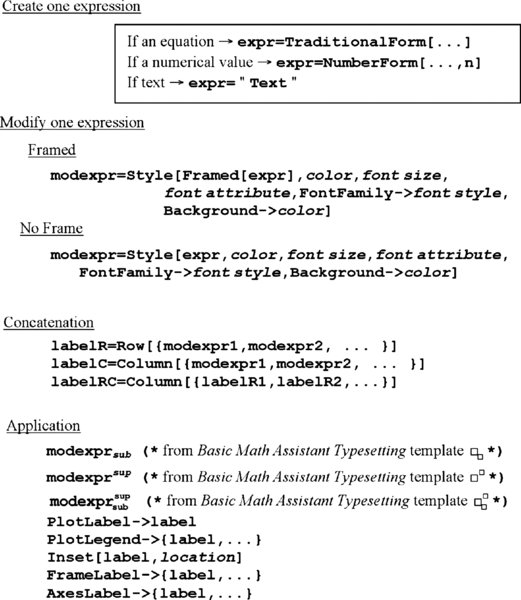
Figure 6.2 General approach to creating labels using Style : color is taken from Table 6.5, and font size, font attribute, and font style are taken from Table 6.7. See Table 6.8 for examples of usage
Axes Characteristics
There are two ways in which axes can appear. The first way is for the axes to appear with tick marks and with tick labels. This is the default way in which axes are displayed. The second way is for the axes to appear without tick marks and without labels and instead the entire figure is framed and the tick marks appear on the inside of the frame and the tick labels appear on the outside of the frame. This option is applied by using the option Frame->True. The characteristics of the axes can be changed as shown in Table 6.9 and those for frames as shown in Table 6.10.
Table 6.9 Options for figure axes
| Axes-> Instruction | ||
| Option | Instruction | |
| Axes drawn | Draw axes (Default) | True or omit the option |
| Omit axes | False | |
| Draw only x-axis | {True,False} | |
| Draw only y-axis | {False,True} | |
| PlotRange-> Instruction | ||
| Option | Instruction | |
| Axes limits | Use all values | All |
| Use most points, omitting outliers | Automatic (default) | |
| Set specific limits | {{xmin,xmax},{ymin,ymax}} | |
| AxesStyle->{{x-axis attribute #1, x-axis attribute #2,…}, {y-axis attribute #1, y-axis attribute #2,…}}* | ||
| Option | x-axis or y-axis attribute | |
| Axes characteristics | Change color of axis, ticks, and tick labels | Color from Table 6.5 |
| Size of tick labels | Font size from Table 6.7 | |
| Tick label style | Font attribute from Table 6.7 | |
| Use default attributes | None or omit the option | |
| Axis thickness | Thickness[…] (see Table 6.6) | |
| Axis dashed | Dashing[…] (see Table 6.6) | |
| AxesLabel->{x-axis instruction, y-axis instruction}† | ||
| Option | x-axis or y-axis instruction | |
| Axes labels (appear at end of each axis) | No label (Default) | {None,None} or omit the option |
| Labels | {labelx,labely}† | |
| Label only x-axis | {labelx,None}† | |
| Label only y-axis | {None,labely}† | |
| Ticks->{x-axis instruction, y-axis instruction} | ||
| Option | x-axis or y-axis instruction | |
| Tick mark characteristics and labels | System decides locations and their labels (default) | Automatic |
| No tick marks | None or omit the option | |
| Specify locations and system determines labels | {loc} = list of x or y coordinates | |
| Specify locations and their respective labels | {{loc1,lab1},{loc2,lab2},…}‡ | |
aIf only one attribute is selected and it is to be applied to both axes, then all braces may be omitted
b labelx and labely are, in general, given by label shown in Figure 6.2.
clocN is either the value of the x-coordinate along the x-axis or the value of the y-coordinate along the y-axis
Table 6.10 Options for figure frames
| Option | Instruction |
| Frame->Instruction | |
| No frame (default) | False or None or omit the option |
| Draw frame on all four sides | True |
| Draw any combination of portions of frame | {{True or False,True or False}, {True or False,True or False}} where the locations are {{left, right},{bottom, top}} |
| FrameLabel-> Instruction | |
| No labels (default) | None or omit the option |
| Label at bottom edge | label* |
| Label at bottom and left edges | {bottom,left} † |
| Label all edges | {{left,right},{bottom,top}}† |
| FrameTicks-> Instruction | |
| No tick marks | None or omit the option |
| Place tick marks automatically | Automatic |
| Place tick marks automatically on bottom and left edges | True |
| Place tick marks automatically on all edges | All |
| Specify locations and labels for each tick mark on each edge | {{left,right}{bottom,top}}† left={{loc1,label1},{loc2,label2},…}‡ or None or Automatic Similarly for right, bottom, and top |
alabel or labelN is given by the general form shown in Figure 6.2
bbottom, top, left, and right specify edge location based on its position in the list; when implemented, an appropriate label of the general form given in Figure 6.2 replaces each of these identifiers
clocN equals x-coordinate value for bottom and top and equals the y-coordinate value for left and right
6.2.3 Common 2D Shapes: Graphics[]
There are several commands that create common 2D shapes. These commands can be used to create separate figures or to enhance a figure. They can also be used to create plot markers as shown in Table 6.15. A list of these shapes is given in Table 6.11. They are created with the following command
Table 6.11 Built-in 2D shapes
| Shape | Mathematica function |
| Lines | Line[{{x1,y1},{x2,y2},…}] |
| Connected lines with the last point containing an arrowhead (unless Arrowheads indicates otherwise) | Arrow[{{x1,y1},{x2,y2},…}] |
| Arrowhead size or size of two arrowheads, one at each end of line | Arrowheads[p] for arrowhead at last point (typically, 0 < p ≤ 0.1) Arrowheads[{-p1,p2}] for arrowheads at first and last points: p1 size of arrowhead of first point (minus sign required), p2 size of arrowhead of last point. Note: must be used to draw two arrowheads and this specification must precede Arrow. |
| Points | Point[{{x1,y1},{x2,y2},…}] |
| Circle or arc of circle | Circle[{x0,y0},r,{ |
| Disk or disk sector | Disk[{x,y},r,{ |
| Ellipse | Disk[{x,y},{rx,ry}] {x,y} = coordinates of ellipse center rx = semi-axis length parallel to x-axis ry = semi-axis length parallel to y-axis |
| Rectangle | Rectangle[{xl,yl},{xu,yu}] {xl,yl} = coordinates of lower left hand corner {xu,yu} = coordinates of upper right hand corner |
| Polygon | Polygon[list] list = list of coordinates of the vertices |
Table 6.12 Additional figure enhancements: see Table 6.13 for typical usage
| Enhancement | Instruction |
| Filling area under a curve, place a line under a point, or place a “volume” under a surface | Filling->loc loc = None ; no filling (default) loc = Axis ; fill to x-axis loc = Top ; fill to top of plot loc = Bottom ; fill to bottom of plot loc = {1->{2}} ; fill between the first and second curves drawn |
| FillingStyle->typ typ = Automatic (default) typ = {col,opa,thk,dash} opa = Opacity[n] (0 ≤ n ≤ 1) col = color from Table 6.5 thk = Thickness[…] from Table 6.6 dash = Dashing[…] from Table 6.6 | |
| Grid lines | GridLines->spec spec = None (default) spec = Automatic spec = {listx,listy}, where listx and listy specify locations of grid lines in each direction: listx or listy can equal None or can equal Automatic |
| Plot title | PlotLabel[label]* |
| Place additional objects on a figure | Epilog->{{obj1},{obj2},…} objN is typically a graphics primitive or an Inset object |
| Rotate a graphics object including an entire figure created by any plot command | Rotate[obj,th,{xo,yo}] obj = object to be rotated th = counterclockwise angle of rotation (radians) {xo,yo} = optional point about which rotation occurs |
alabel is, in general, of the form given in Figure 6.2.
Table 6.13 Examples of graph enhancement using the options listed in Table 6.12
| h[t_,p_]:=Exp[-0.15 t] Sin[t-p];
gx=Table[g,{g,Range[1,15,1]}]; (* Coordinates of grid lines for
x-axis *)
lab=Style["Two curves",Blue];
eq=Table[{n,h[n,0]},{n,2. |
|
options: PlotLabel->lab |
options: PlotLabel->lab,
Filling->{1->{2}},
FillingStyle->Orange,
Frame->True |
options: PlotLabel->lab,
Filling->{1->{2}},
FillingStyle->Orange,
Frame->True,
GridLines->{gx,Automatic} |
options: PlotLabel->lab,
Filling->{1->{2}},
FillingStyle->Orange,
Frame->True,
GridLines->{gx,Automatic},
Epilog->{PointSize[0.02],
Yellow,Point[eq]} |
| Rotate[p1, |
 |
a Coordinates of curves’ intersections
Table 6.14 Graph enhancement using legends
| plt=Sequence[{BesselJ[0,x],Exp[-(x-4)^2/2]},{x,0,10}]; lst1=Table[{x,BesselJ[0,x]},{x,Range[0,10,0.15]}]; lst2=Table[{x,Exp[-(x-4)^2/2]},{x,Range[0,10,0.15]}]; pstyl=Sequence[PlotStyle->{{Dashing[{}],Black},{Dashing[Medium],Blue}}]; lstl=Sequence[{TraditionalForm[BesselJ[0,x]],TraditionalForm[Exp[-(x-4)^2/2]]}]; frd=Sequence[{RoundingRadius->10,Background->Yellow,FrameStyle->Blue}]; | |
Plot[Evaluate[plt],Evaluate[pstyl], PlotLegends->Placed["Expressions",Right]] |
Plot[Evaluate[plt],Evaluate[pstyl], PlotLegends->Placed[LineLegend[ {"Bessel","Exponential"}],Right]] |
Plot[Evaluate[plt],Evaluate[pstyl],PlotLegends-> Placed[LineLegend["Expressions", LegendLabel->"Functions"],Right]] |
Plot[Evaluate[plt],Evaluate[pstyl], PlotLegends->Placed[LineLegend["Expressions", LegendLabel->"Functions", LegendFunction->Framed],Right]] |
Plot[Evaluate[plt],Evaluate[pstyl], PlotLegends->Placed["Expressions",Top]] |
Plot[Evaluate[plt],Evaluate[pstyl], PlotLegends->Placed[LineLegend["Expressions", LegendLabel->"Functions",LegendFunction-> (Framed[#,Evaluate[frd]] &)],Right]] |
ListLinePlot[{lst1,lst2},PlotLegends-> Placed[LineLegend[Sequence[lstl], LegendLabel->"Functions"],Right]] |
ListPlot[{lst1,lst2},PlotLegends-> Placed[PointLegend[Sequence[lstl], LegendLabel->"Functions"],Right]] |
ListLinePlot[{lst1,Legended[lst2, TraditionalForm[Exp[-(x-4)^2/2]]]},PlotLegends-> Placed[LineLegend[None,LegendLabel->"Function", LegendFunction->Framed],Right]] |
ContourPlot[Sin[2 x] Sin[y],{x,0,1},{y,0,1}, ColorFunction->ColorData["Rainbow"], PlotLegends->Placed[BarLegend[Automatic], Right]] |
Plot[Evaluate[plt],Evaluate[pstyl], PlotLegends->Placed["Expressions",{0.8,0.8}]] |
|
Table 6.15 Examples of using PlotMarkers and Filling
| Objective | Program* | Output |
| Use default values | lst1=Table[{n |
 |
| Use default values | lst1=Table[{n |
 |
| Select fill and marker characteristics | lst1=Table[{n |
 |
| Place a series of points whose locations differ from those used to plot curve | lst1=Table[{n |
 |
| Place different markers at same x location | lst1=Table[{n |
 |
aAdditional plot marker shapes, which include the shapes shown above, can be obtained by using Polygon and symbols from the palette shown in Figure 1.2b.
Graphics[{s1,s2,…c1,c2,…},opt]
where opt are options such as Axes and Frame that can be used to further modify the figure and
sK={col1K,EdgeForm[{col2K,thkK,dashK}],shape,Opacity[n]}
cK={colK,thk,dash,cla}
In these expressions,
- colK, col1K, and col2K are colors from Table 6.5;
- thkK, thk = Thickness[…] specifies the line thickness as shown in Table 6.6;
- dashK, dash = Dashing[…] specifies a dashed line as shown in Table 6.6;
- Opacity[n] is the degree of opaqueness, where n is a number from 0 to 1 with 1 being opaque and 0 being invisible: default is opaque.
- shape = Disk (Ellipse), Rectangle, or Polygon
- cla = Circle, Line, Point, or Arrow
- EdgeForm controls the properties of the perimeter of the shape
With regard to Point, the options dash and thk are replaced with
PointSize[arg]
where arg is either Tiny, Small, Medium, Large, or a decimal number that typically is in the range 0 < p ≤ 0.1.
The usage of these shapes is illustrated with the following statement
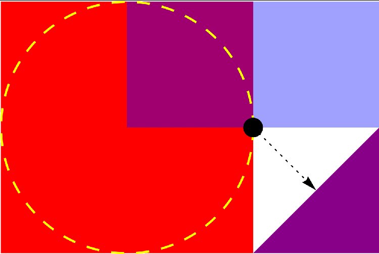
Figure 6.3 Application of several built-in 2D shapes
Graphics[{{Red,Rectangle[{0,0},{1,1}]},
  {Blue,Opacity[0.4],Rectangle[{0.5,0.5},{1.5,1}]},
  {Thick,Yellow,Dashing[Large],Circle[{0.5,0.5},0.5]},
  {Purple,Polygon[{{1,0},{1.5,0},{1.5,0.5}}]},
  {Dashing[Small],Arrow[{{1,0.5},{1.25,0.25}}]},
  {Black,PointSize[0.05],Point[{1,0.5}]}}]
the execution of which yields Figure 6.3.
For another illustration, two of these built-in shapes are used to create n concentric circles and n concentric unfilled rectangles as follows. It is assumed that the rectangle and the circle are centered at (xc,yc), the width of the rectangle is a and its height is b, and the radius of the circle is r. The coordinates of the end points of the rectangle in terms of xc and yc are given by (xc − na/2, yc − nb/2) for the lower left corner and by (xc + na/2, yc + nb/2) for the upper right corner, where n = 1, 2, … , is the number of rectangles to be drawn. If it is assumed that xc = 1, yc = 1, b = 0.5, a = r and r varies from 0.5 to 2 in increments of 0.5, then the program to draw these concentric shapes is
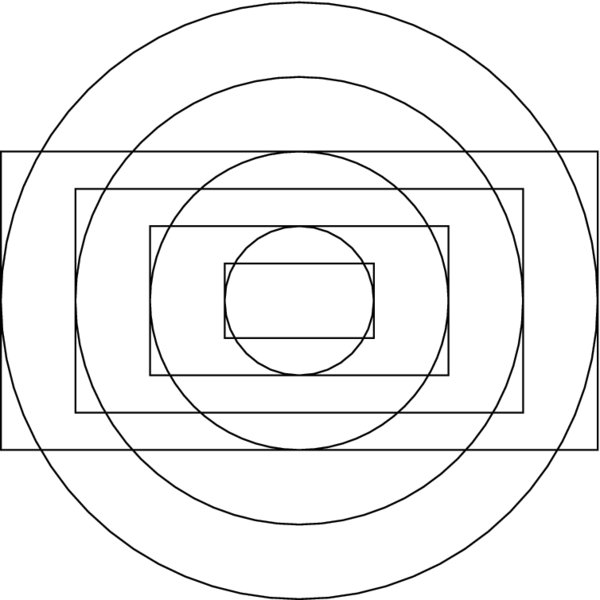
Figure 6.4 Concentric circles and concentric rectangles using built-in 2D shapes
xc=1;    yc=1;    a=1;    b=0.5;
Graphics[{Table[{EdgeForm[Black],Opacity[0.],
  Rectangle[{xc-n a/2,yc-n b/2},{xc+a n/2,yc+b n/2}]},
   {n,1,4}],
  Table[Circle[{xc,yc},r],{r,0.5,2,0.5}]}]
where we have used EdgeForm to define the perimeter of the rectangle independently of the rectangle’s opaqueness, which has been set to 0 (invisible). The execution of this program produces Figure 6.4.
6.2.4 Additional Graph Enhancements
In addition to the enhancements described above, there are several other enhancements that are often used to increase the visual impact of a figure. These are: filling regions under curves, drawing grid lines, placing additional objects within the figure, placing a figure title, and rotating the figure. Typical objects are text, graphics shapes, or another figure. These figure enhancements are listed in Table 6.12 and illustrated in Table 6.13.
Legends
The basic legend commands that are introduced are: PlotLegend s, which creates legends; LegendLabel, which places a title over the legends; LineLegend, which selects the characteristics of the legend identifiers such as line colors and their labels; and LegendFunction, which specifies the characteristics of the box that contains the legends. To have additional flexibility when using legends, two additional commands are often employed. The first is
Placed[expr,{xp,yp}]
which places expr at the location {xp,yp}. The magnitude of {xp,yp} is a function of the command in which it is used. For graphs, it is typically a pair of positive numbers between 0 and 1. The second command is
Legended[expr,label]
which, when used with the appropriate legend commands, will associate label with expr. It is used when only selected curves are to be identified in a legend.
Examples of the use of these commands are given in Table 6.14 for Plot, ListPlot, ListLinePlot, and ContourPlot. In addition, to improve readability of the programs in Table 6.14, the command
Sequence[arg]
is used. The quantity arg represents a sequence of comma-separated arguments that can be placed into any function. In Table 6.14, it is used to specify the characteristics of line and point styles of the graphs and is implemented with Evaluate.
Plot Markers
Plot markers are a way to specify the shape and size of the symbol used to plot the data values that appear in the ListPlot family of plotting functions. The basic option is
PlotMarkers->Automatic
To specify a specific shape, color, and size of the plot marker, the following is used
PlotMarkers->{Graphics[{color,shape}],n}
wherecolor is a the color selected from Table 6.5, shape is a graphic shape selected from Table 6.11, and n is a number, a typical value of which is 0.03. Examples of the usage of PlotMarkers are given in Table 6.15.
Placement of an Object within a Figure
One or more objects can be placed anywhere in a figure by using Epilog, Insert, and the definitions in Figure 6.5. The Inset command is
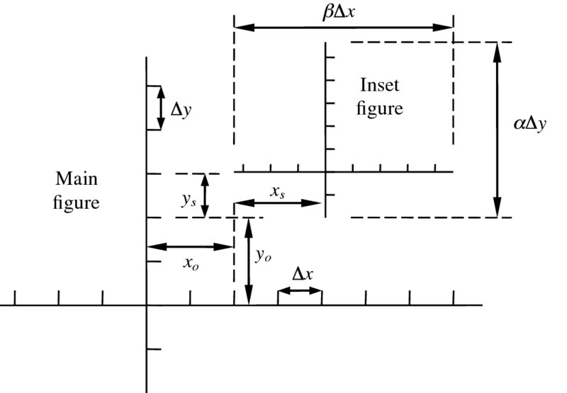
Figure 6.5 Definitions of the parameters used by Inset for placement of a figure within a figure
Inset[obj,loc]
where obj is a graphics object or text, loc = {xo,yo} is the location where the center of the object’s coordinate system will be placed, sft={xs,ys} is the location with respect to the inserted figure’s coordinate system, and sz={ ![]() Δx,
Δx,![]() Δy}. When used with LogPlot, LogLinearPlot, and LogLogPlot, the following transformation has to be performed on the location coordinates:
Δy}. When used with LogPlot, LogLinearPlot, and LogLogPlot, the following transformation has to be performed on the location coordinates:
LogPlot → loc = {x1,Log[y1]}
LogLinearPlot → loc = {Log[x1],y1}
LogLogPlot → loc = {Log[x1],Log[y1]}
As an example, consider following statements

Figure 6.6 Illustration of Inset that placed a figure within a figure
p2=Plot[2-x^2-x^3,{x,-1,1}];
Plot[2+x^2+x^3,{x,-2,2},PlotRange->All,
  Epilog->Inset[p2,{-1,6},{0,0},{8,8}]]
which produces Figure 6.6.
These graph enhancement techniques are now illustrated with the following examples.
Table 6.16 Output of Example 6.1 as a function of plot enhancements
| Plot[h[x],{x,-1,2},PlotRange->{{-1,2},{-10,100}},options] opt1=Sequence[PlotLabel->plab,Filling->Axis,FillingStyle->Orange]; opt2=Sequence[AxesLabel->{"x","h(x)"},LabelStyle->{14,Blue}]; opt3=Sequence[{PointSize[Large],Point[{xmin,hmin}]}]; opt4=Sequence[{Dashing[Medium],Line[{{0,hmax},{1.5,hmax}}]}, {Arrowheads[0.03],Arrow[{{0.7,80},{xmax,hmax}}]}, Inset[hminlab,{0.8,7.}],Inset[hmaxlab,{0.4,80}]]; | |
options:none |
options: Evaluate[opt1] |
| options: Evaluate[opt1], Evaluate[opt2], Epilog->{Evaluate[opt3]} | options: Evaluate[opt2], Evaluate[opt2], Epilog->{Evaluate[opt3], Evaluate[opt4]} |
 |
 |
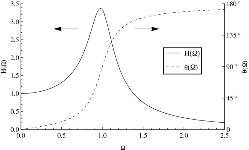
Figure 6.7 Results from Example 6.2
Figure 6.8 Results from Example 6.3
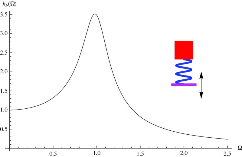
Figure 6.9 Insertion of a representation of a base-excited spring–mass system using graphics primitives
6.2.5 Combining Figures: Show[] and GraphicsGrid[]
The command Show allows one to combine several graphical entities into one figure, including the combination of those created with different plotting commands such as Plot and ListPlot. However, the major labeling and overall appearance of the final graphic will be determined by the first plotting or graphics command appearing in Show. Therefore, one should place the desired overall graphic options in this command.
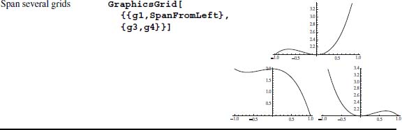
Show combines several distinct graphs onto one graph. If one wants to keep several distinct graphs separate, but arrange them in a specific manner based in some sort of grid, then there are three other commands to perform this function. The first command is GraphicsGrid, which arranges the graphs on an n × m grid. The second is GraphicsColumn, which place the graphs in a column one below the other. The third command is GraphicsRow, which places the graphs adjacent to each other in a row. These commands and their respective output are illustrated in Table 6.17.
Table 6.17 Various ways of grouping individual figures into one figure entity

The use of Show is illustrated with the following example.
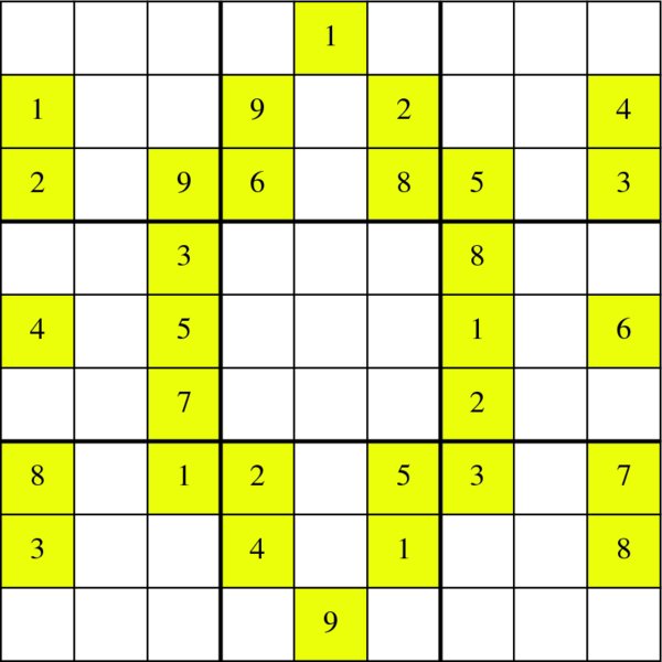
Figure 6.10 Sudoku grid with yellow squares highlighting the initial values and thick lines delineating the 3 × 3 sub arrays

Figure 6.11 Example of (a) a default contour plot; (b) modified contour plot shown in (a)
6.2.6 Tooltip[]
Tooltip is a graph enhancement that allows one to use a mouse pointer to display information about curves or data points when the mouse pointer is over a curve or a data point. Its form is
Tooltip[expr,label]
where label will be displayed in a framed box. The use of Tooltip in plotting is shown in Table 6.18.
Table 6.18 Examples of ToolTip usage
| Tooltip objective | Instructions | Figure* |
| Identify each curve | c1=Tooltip[Sin[x],
TraditionalForm[Sin[x]]];
c2=Tooltip[Cos[2 x],
TraditionalForm[Cos[2 x]]];
Plot[{c1,c2},{x,0,5 |
 |
| Display values of individual data points [unformatted] | lst1=Table[Tooltip[{x,Sin[x]}],
{x,Range[0,5. |
 |
| Display values of individual data points [formatted] | lst1=Table[Tooltip[
{x,Sin[x]},Column[{Row[{"x = ",
NumberForm[x,3]}],
Row[{"sin(x) = ",
NumberForm[Sin[x],3]}]}]],
{x,Range[0,5. |
 |
| Display values of individual data points and connect data points [unformatted] | ListLinePlot[Table[Tooltip[
{x,Sin[x]},{x,Sin[x]}],
{x,Range[0,5. |
 |
| Display values of individual data points, connect data points, and identify data set [unformatted] | lst1=Table[Tooltip[{x,Sin[x]},
Column[{"Data set #1",
{x,Sin[x]}}]],
{x,Range[0,5. |
 |
aArrow indicates cursor position and text in box is produced by Tooltip. For graphs with two curves, both tooltips are shown; however, in actuality, only one can appear at a time.
bPlotmarkers is required otherwise Tooltip will not appear.
6.2.7 Exporting Graphics
Graphic entities can be saved to a directory of choice and in one of several formats by using Export. Its form is
Export["Path/FileName.ext",fig,"Graphics"]
where Path is the directory where the graphic is to reside, FileName is the file name that the user gives to the graphic, .ext is the extension to the file name that dictates the form in which the graphic is to be saved such as .eps, .tif, and .jpg, and “Graphics” is one of several descriptors that is used to define the type of graphic/image that is being exported. The quantity fig represents the graphic or image to be exported. It can be the graphic or image itself or a symbol defined by the figure.
6.3 3D Graphics
There are numerous three-dimensional plotting functions that are available in Mathematica. The ones that we shall discuss are listed in Tables 6.19. The plotting can be enhanced in the same manner that the 2D plotting functions were; that is, one may use the options appearing in Tables 6.5, 6.6, 6.7, 6.9, 6.12, and 6.18. However, there are three additional commands that are specific to 3D graphs: Boxed, Mesh, and ViewPoint. These are listed in Table 6.20. Also, for 3D graphics, one can rotate the display interactively by placing the cursor over the figure. A pair of curved lines, each with an arrowhead appearing head to tail, will become visible. Depressing the mouse button and moving this cursor will cause the figure to change orientation.
Table 6.19 3D plotting commands for plotting surfaces
| Plotting type | Mathematica function |
| Basic | Plot3D[{f,g,…},{x,xs,xe},{y,ys,ye}] f = f(x,y), g = g(x,y), … are the z coordinates of the surfaces for xs ≤ x ≤ xe and ys ≤ y ≤ ye |
| Parametric | ParametricPlot3D[{f,g,h},{u,us,ue},{v,vs,ve}] f = f(u,v), g = g(u,v), and h = h(u,v) are the (x,y,z) coordinates of a point on the surface |
| Surface of revolution | RevolutionPlot3D[{fr,gz},{t,ts,te},{th,ths,the}] fr = f(t) is the radial coordinate value at t for ts ≤ t ≤ te gz = g(t) is the value of z at a value of t for ts ≤ t ≤ te th = angle of rotation of fr and gz starting at ths and ending at the |
| List of values | ListPlot3D[{{x1,y1,f1},{x2,y2,f2},…}] fN = f(xn, yn) = value of the z-coordinate corresponding to xn = xN and yn = yN |
Table 6.20 Additional options for three-dimensional graphics: see Table 6.22 for typical usage
| Boxed-> Instruction | ||
| Option | Instruction | |
| Bounding box | Draw box (default) | True |
| Omit box | False | |
| Mesh-> Instruction | ||
| Option | Instruction | |
| Mesh | Draw mesh (default, using n = 15) | True (or Mesh omitted) |
| Omit mesh | False | |
| Draw mesh using all regular points | Full | |
| Draw n equally spaced meshes | Positive integer | |
| ViewPoint-> Instruction* | ||
| Option | Instruction | |
| View point | Default | {1.3,-2.4,2} |
| Top | Top | |
| Bottom | Bottom | |
| Front | Front | |
| Back | Back | |
| Left | Left | |
| Right | Right | |
| Combined | {Top,Front},{Top,Left}, etc. | |
aThere are numerous ways to invoke this option; see ViewPoint in Documentation Center for other choices
As was the case for 2D graphics, Mathematica provides commands that can create common 3D objects. These commands can be used to create separate figures or to enhance a figure. A list of these shapes is given in Table 6.21. They are created with the following command
Table 6.21 Three-dimensional shapes
| Shape | Mathematica function |
| Connected lines | Line[{{x1,y1,z1},{x2,y2,z2},…}] |
| Connected lines with the last point containing an arrowhead | Arrow[{{x1,y1,z1},{x2,y2,z2},…}] |
| Points | Point[{{x1,y1,z1},{x2,y2,z2},…}] |
| Polygon | Polygon[{{x1,y1,z1},{x2,y2,z2},…}] {xN,yN,zN} = coordinates of vertices |
| Cone | Cone[{{x1,y1,z1},{x2,y2,z2}},r] {x1,y1,z1} = location of center of base {x2,y2,z2} = location of tip of cone r = radius of base |
| Cylinder | Cylinder[{{x1,y1,z1},{x2,y2,z2}},r] {x1,y1,z1} = location of center of one end of cylinder {x2,y2,z2} = location of center of the other end of cylinder r = radius of cylinder |
| Cuboid (rectangular parallelepiped) | Cuboid[{xl,yl,zl},{xu,yu,zu}] {xl,yl,zl} = coordinates of lower left-hand corner of cuboid {xu,yu,zu} = coordinates of upper right-hand corner of cuboid |
| Sphere | Sphere[{x1,y1,z1},r] {x1,y1,z1} = location of center of sphere r = radius of sphere |
| Tube (connected lines made into a cylindrical tube) | Tube[{{x1,y1,z1},{x2,y2,z2},…},r] r = radius of the tube |
Graphics3D[{s1,s2,…c1,c2,…},opt]
where opt are options such as Axes, Mesh, Boxed, ViewPoint, and MaxRecursion that can be used to modify the figure and
- sK={col1K,EdgeForm[{col2K,thkK,dashK}],Opacity[n],shape}
- cK={colK,thk,dash,pla}
- colK, col1K, col2K = color from Table 6.5
- thkK = Thickness[…] : line thickness from Table 6.6
- dashK = Dashing[…] : dashed lines from Table 6.6
- Opacity[n] = degree of opaqueness: n is a number from 0 to 1, where 1 is opaque and
0 is invisible. If omitted, the shape is opaque. - shape = Cone, Cuboid, Cylinder, Sphere, or Tube
- pla = Point, Line, Polygon, or Arrow
In addition to the 3D shapes listed in Table 6.21, one can create a three-dimensional object of arbitrary complexity by using
GraphicsComplex[vec,prim]
where vec is a list of K triplets of numbers and prim denotes the connectivity of the vertices of the object. Thus,
vec={{x1,y1,z1},{x2,y2,z2},…{xK,yK,zK}};
The argument of prim is a list of lists of integers, with each integer corresponding to a point in vec. The order of these integers is used by ComplexGraphics to create a surface with these vertices for each element of prim. For example,
prim[{{1,2,5,6},…}
indicates that the vertices of the first implementation of prim is composed of the points connected in the order given; that is,
{{x1,y1,z1},{x2,y2,z2},{x5,y5,z5},{x6,y6,z6}};
To illustrate the use of this command, we shall create a frustum of a right pyramid whose base is 1 by 1 units and whose top is 0.25 by 0.25 units and 2 units from the base. This object consists of six 4-sided polygons and its creation, which is shown in Figure 6.12, is obtained from
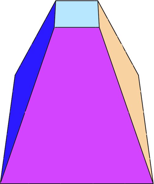
Figure 6.12 Frustum of a right pyramid created with GraphicsComplex
vec={{0,-1/4,-1/4},{0,1/4,-1/4},{0,1/4,1/4},{0,-1/4,1/4},
  {2,-1,-1},{2,1,-1},{2,1,1},{2,-1,1}};
n={{1,2,3,4},{5,6,7,8},{1,2,6,5},{3,4,8,7},{1,4,8,5},
  {2,3,7,6}};
Graphics3D[{Opacity[1],GraphicsComplex[vec,Polygon[n]]},
  Boxed->False,ViewPoint->{Bottom,Left}]
The detailed characteristics of a three-dimensional shape can be significantly altered by the options selected. To give an indication of how these options can alter a three-dimensional figure, we have chosen to show the effects of several of them on the parametric surface

for 0 ≤ u ≤ 2π, −15 ≤ u ≤ 6, a = 1.13, and b = 1.14. The program that displays this shape is given in Table 6.22 as a function of several options.
Table 6.22 Illustration of the effects of several 3D graphics options
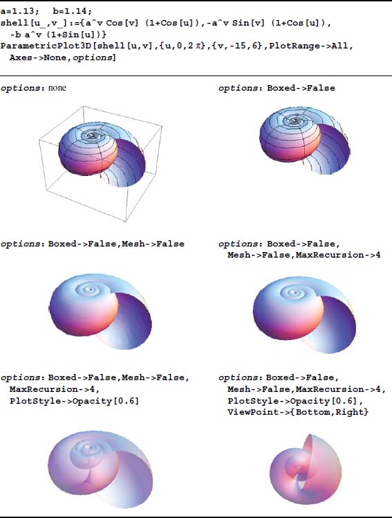
We shall now illustrate the use of the three-dimensional plot commands appearing in Tables 6.19 to 6.21. ParametricPlot3D has been illustrated in Table 6.22. The following examples illustrate the use of Graphics3D, Plot3D, ListPlot3D, and RevolutionPlot3D.
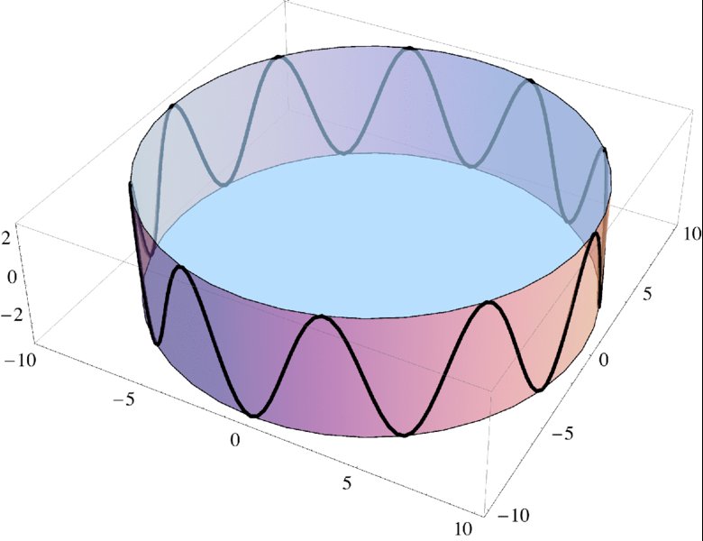
Figure 6.13 Sine wave on the surface of a cylinder
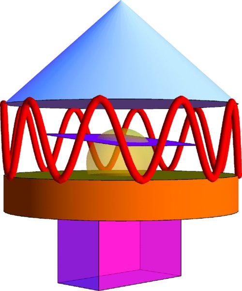
Figure 6.14 Arbitrary arrangement of built-in 3D shapes

Figure 6.15 Intersection of two surfaces and the use of Filling
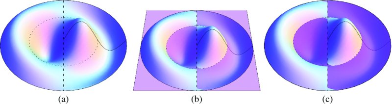
Figure 6.16 Mode shape of a clamped circular membrane where dashed lines indicate locations of nodal circle and nodal diameter: (a) no horizontal plane; (b) with horizontal plane; (c) with horizontal plane represented by a very thin cylinder

Figure 6.17 Surface of revolution created by the rotation of a generatrix through 3π/2 radians
6.4 Summary of Functions Introduced in Chapter 6
The 2D plot commands are listed in Tables 6.1 to 6.4 and the built-in 2D geometric shapes are listed in Table 6.11. The options that are available to these graphics commands are listed in Tables 6.5, 6.6, 6.7, 6.9, 6.10, 6.12, 6.14, 6.15, and 6.18. The 3D plotting functions are given in Table 6.19 and the options specific to 3D graphics are listed in Table 6.20. The built-in 3D geometric shapes are listed in Table 6.21.
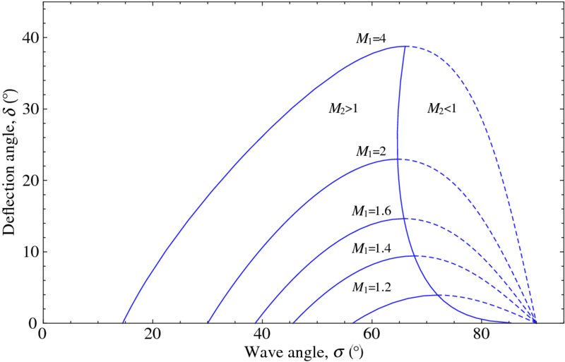
Figure 6.18 Solution to Exercise 6.1
References
- P. K. Kundu and I. M. Cohen, Fluid Mechanics, 4th edn, Academic Press, Burlington, Massachusetts, 2008, p. 753.
- E. W. Weisstein, CRC Concise Encyclopedia of Mathematics, 2nd edn, Chapman Hall/CRC, Boca Raton, 2003, p. 2129–30.
- A. Leissa, Vibration of Shells, NASA Sp-288, 1973, p. 44.
- F. P. Incropera and D. P. Dewitt, Introduction to Heat Transfer, 4th edn, John Wiley & Sons, New York, 2002, p. 675.
Exercises
Section 6.2
- 6.1 The relationship between an oblique shock wave at an angle σ and the deflection angle δ as a function of the incident Mach number M1 is [1]
where γ is the ratio of the specific heats of the gas. For a given M1, there is a value of σ for which δ is a maximum. We denote these values as σmax and δmax. Then for a given M1 those values of σ > σmax for which δ < δmax the downstream Mach number M2 is less than 1 and the shock waves are called strong shock waves. For those values σ < σmax for which δ < δmax, the downstream Mach number M2 is greater than 1 and the shock waves are called weak shock waves. With this information, use Eq. (6.1) to obtain Figure 6.18. This figure was obtained with γ = 1.4.
- 6.2 For a given value of y, the value of p is determined from

where h = 10−p, k1 = 2.5 × 10⁻⁴, k2 = 5.6 × 10⁻¹¹, and k3 = 1.7 × 10⁻³. Plot the value of p when 0.00001 ≤ y ≤ 2.5.
- 6.3 The Cartesian locations of bi-cylinder coordinates are given by
If a = 1.5, −1 ≤ η ≤ 1, and 0 ≤ ϕ ≤ 2π, replicate Figure 6.19.
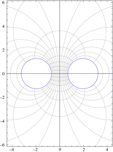
Figure 6.19 Solution to Exercise 6.3
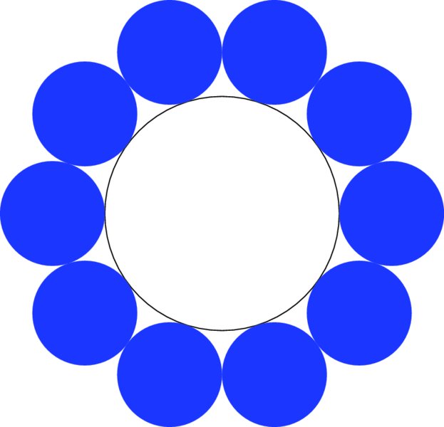
Figure 6.20 Solution to Exercise 6.4
- 6.4 One can draw n circles, n ≥ 3, that are tangent to a central circle of radius rb and to each adjacent circle as shown in Figure 6.20 for n = 10. The radius of the outer circles is

Write a program that replicates this figure and similar figures for arbitrary n. In this case, the outer circles (disks) are blue.

Figure 6.21 Solution to Exercise 6.5
- 6.5 A Pappus chain is a series of n tangent circles inscribed in the area between three semicircles as shown in Figure 6.21. The radius of the outer circle is Ro and the radii of the other two circles are RL and RR, RL ≥ RR. The location of the center of the nth circle is [2]

and its radius is

where r = 2RL/(RL + RR). The ellipse that connects the centers of the circles is given by
Replicate Figure 6.21, which has been obtained for n = 4, Ro = 1/2, RL = 1/4, and RR = 1/4. Color the four complete circles yellow and their background green. The right semicircle is colored magenta and the left one red.
- 6.6 A piece-wise linear map is defined by the points with the coordinates

Obtain a plot for the coordinate points when x1 = 1, y1 = 3.65, and N = 15,000. The resulting figure is sometimes referred to as the gingerbread man.
- 6.7 The following relation is used to determine the value of a pipe’s coefficient of friction λ for a given Reynolds’ number Re, pipe diameter d, and surface roughness k
Using this relation, replicate Figure 6.22.
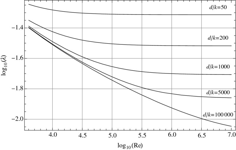
Figure 6.22 Solution to Exercise 6.7

Figure 6.23 Solution to Exercise 6.8
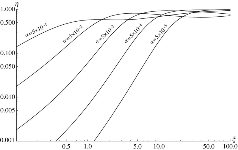
Figure 6.24 Solution to Exercise 6.9
- 6.8 The following equation will plot a Joukowsky airfoil over the range −0.5 ≤ x ≤ 0.5

where the plus sign describes the top of the airfoil and the negative sign its bottom. With h = 0.08 and t = 0.13, replicate the Figure 6.23.
- 6.9 A normalized structural damping factor describing the losses in a vibrating thin plate with a damping layer is given by
where α is the ratio of the layers’ moduli and ξ is the ratio of the layers’ thickness. Replicate the logarithmic plot shown in Figure 6.24. The x-locations of the curves’ labels and their individual orientations have been done iteratively.
- 6.10 Given the following polynomial [3]
where

For ν = 0.3, h = 10−5, and n = 1, 2, 3, 4, 5, plot the smallest positive value of Ω that satisfies Eq. (6.2) for 0.5 ≤ π/λ ≤ 100. The results should look like those shown in Figure 6.25. The placement of the labels on the curves should appear as shown even if the value of h changes.

Figure 6.25 Solution to Exercise 6.10

Figure 6.26 Solution to Exercise 6.11
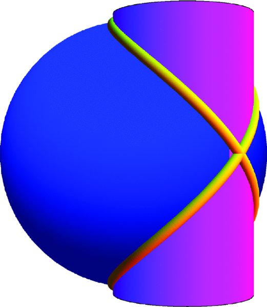
Figure 6.27 Solution to Exercise 6.14
- 6.11 The spectral emissive power is given by the Planck distribution [4]

where c1 =3.742 × 10⁸ W μm4·m−2 and c2 = 1.4388 × 104 μm K. For T = {2000., 1000., 400., 100.} K, obtain a plot of E versus λ. The result should look like that shown in Figure 6.26. Show in tabular form that for the four temperatures given, λmaxTn = 2898 μm K.

Section 6.3
- 6.12 Plot the surface described by
over the region indicated. Label the axes.
- 6.13 Plot the surface described by
over the region indicated when a = 0.25. Label the axes.
- 6.14 The curve that results from the intersection of a sphere of radius 2a centered at the origin and a cylinder of radius a centered at (a,0,0) is given by the parametric equations

where 0 ≤ ϕ ≤ 4π. If a = 1 and the length of the cylinder is 2, then replicate Figure 6.27. Use a tube radius of 0.04. Color the sphere blue, the cylinder magenta, and the tube yellow.
- 6.15 Plot the following parametric equations over the regions indicated.
- Figure eight torus

- Seashell
- Astroidal ellipsoid
- Figure eight torus