7
Interactive Graphics
7.1 Interactive Graphics: Manipulate[]
The Manipulate command is a straightforward way create an interactive environment for the manipulation of the parameters u1, u2, … of an expression f(x, y, u1, u2, …). The output of Manipulate can be numbers, symbolic expressions, and graphics. The Manipulate command has a very wide range of interactive capabilities. We shall discuss several of them in detail and follow their introduction with examples.
To illustrate the capabilities of Manipulate, the following general form is assumed
  Manipulate[expr,
    text1,
    Item[object1,pos1]
    {spec1},
    Delimiter,
    text2,
    Item[object2,pos2]
    {spec2},
    Delimiter,
    …,
    ControlPlacement->{pl1,pl2,…},
    Initialization:>(proc),
    SaveDefinitions->True
    TrackedSymbols:>{u1,u2,…}]
Each of these terms will be discussed in what follows.
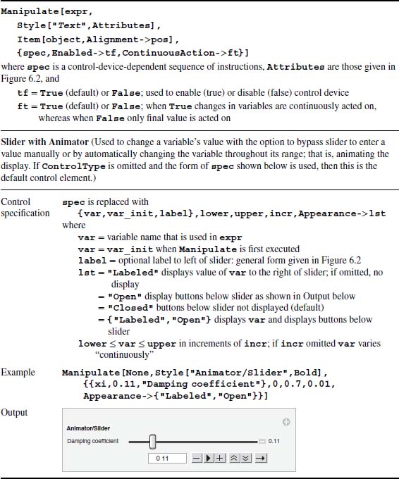
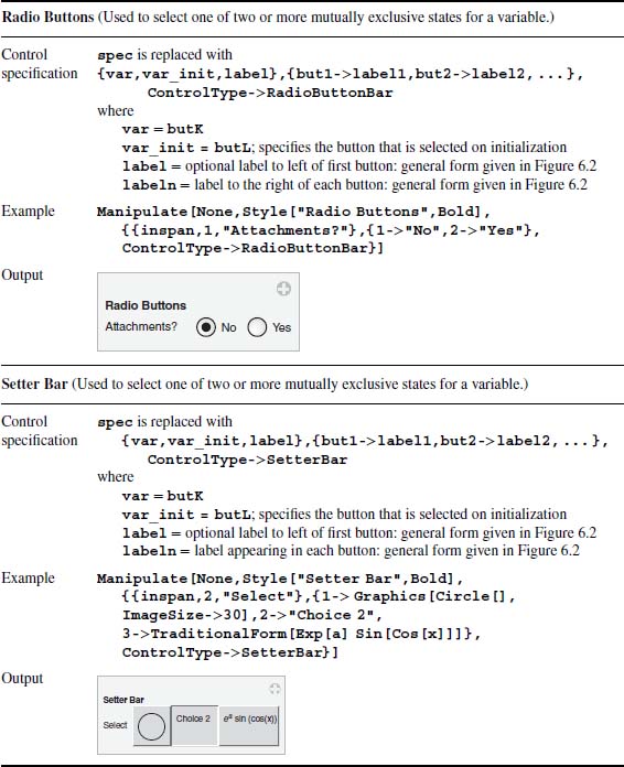
The Manipulate command creates two types of output. In our case, the first type will be primarily a graphical display of the results, which can be composed of one or more fully annotated figures with each figure containing one or more curves. The procedure to create the graphic is denoted expr, which represents f(x, y, u1, u2, …). If more than one expression is used to create expr, then each expression is terminated with a semicolon, except for the last expression, which is terminated with a comma. The second type of output is a set of control devices that provide the interactivity; that is, the ability to change the parameters u1, u2, …, (denoted uN) that appear in f(x, y, u1, u2, …). The control devices that we shall consider are the slider/animator, slider, 2D slider, radio buttons, setter buttons, popup menu, locator, angular gauge, and horizontal gauge. Each of these control devices requires a different set of specifications (denoted specN, and that is a function of uN) and can appear in any order after expr. The specifications for each of these control devices are presented in Table 7.1 along with examples of their respective usage. Each control device specification can be intermixed with: optional text display, which is denoted by textN ; the optional command Item, which is used to place a Mathematica-generated object such as a graphic or equation or to place an imported image from an external source; and the optional use of Delimiter, which places a horizontal line to visually delineate text or a control device or a group of control devices. One can employ any number of the control devices as are meaningful and these control devices need not be different. It will be seen that the slider tends to be used most often. In the general form depicted above, textN is usually given by the general form shown in Figure 6.2; that is, by Style["Message", color, font style, font attribute]; the form "Message" without using Style can also be used.
Table 7.1 Several Manipulate control devices, their usage, and their representative output


The command Item is given by
Item[object,Alignment->pos]
where object is the object to be placed and pos is the position of the object: Left (default), Right, or Center. The object can be a graphic generated with Mathematica commands as illustrated in the subheading Item in Table 7.1, or it can be a picture in one of many formats.
After the control elements have been specified, there are numerous options that are available. Four that are frequently employed are now introduced. The first is
ControlPlacement->{pl1,pl2,…}
which is used to position each control device and each message (textN) with respect to the output area in the order that they appear. If omitted, the control devices are placed at the top. The value of each plN can be Left, Right, Top, or Bottom. If only one position is selected, then all control devices are placed at that location.
The second option is
Initialization:>(proc)
where proc is a procedure that, with respect to expr, can contain any constants that need to be given values, any solutions to one or more equations that need to be obtained, any data sets that need to be initialized, and any functions that need to be created. In addition, it can contain any figures that must be created or inserted prior to using Item. Each of the types of operations would be contained in proc and would be of the form (c1=operation1; c2=operation2; …), where operationN is a specified operation needed to evaluate or define or assign a value to cN. The parentheses are required if there is more than just c1. The usage of Initialization is illustrated in Table 7.1 under the subheading Item.
The third option is
TrackedSymbols:>{u1,u2,…}]
which is used to specify which parameters appearing in the control device definitions should trigger updates when changed. It is a list of the parameter names u1, u2, . . . . It is good practice to always use TrackedSymbols.
The fourth option is
SaveDefinitions->True
which is needed when converting a notebook that contains Manipulate to a CDF file. It ensures that all data sets and function definitions are embedded in Manipulate prior to its conversion. Although this function is typically performed by Initialization, in some cases the amount of data and/or the number and complexity of the function definitions may make their inclusion in Initialization awkward or inconvenient. In this case, one does two things. The first is to place the data and function definitions prior to Manipulate but in the same cell. The second is to employ the option statement shown above.
We shall discuss in a little more detail the animator/slider presented in Table 7.1. This control device is the most capable of all the control devices. Referring to the example output of this device shown in Table 7.1, clicking on the minus sign to the right of the slider bar removes the display of the symbols under the slider. The minus sign now becomes a plus sign; clicking on it will again display these symbols. The box that contains the number 0.11 can be used to enter a numerical value manually. If the value 0.25 is typed and Enter is pressed, the new value for var will be 0.25 and 0.25 will appear at the right of the slider. If the number entered is greater than upper or less than lower, the number will be used in the evaluation of expr, but the appropriate end of the slider will turn red, indicating that a limit has been exceeded.
The six buttons under the slider will now be discussed. The “−” button will decrement the current value of var by incr, whereas the “+” button will increment the current value of var by incr. Clicking on the button with the solid triangle will cause the slider to assume all values of var between lower and upper sequentially at a given rate, thereby creating an animation of the image with respect to that variable. Each new value of var is obtained by adding/subtracting incr to it. Clicking on this button, which now displays two parallel bars, will stop this calculation. Whether the continuous calculation is adding or subtracting incr depends on the direction of the arrow of the right-most button. When the arrow is pointing to the right (→) it will be adding incr, when it is pointing to the left (←) it will be subtracting it, and when the arrow is pointing in both directions (↔) it will add it until it reaches the maximum value and then subtract it until it reaches its minimum value and continue in this fashion until stopped. Lastly, the rate at which the continuous calculations occur can be increased or decreased, respectively, by clicking one or more times on the button with the two upward pointing arrowheads and can be decreased by clicking one or more times on the button with the downward pointing double arrowheads.
The use of Manipulate is now illustrated with several examples.
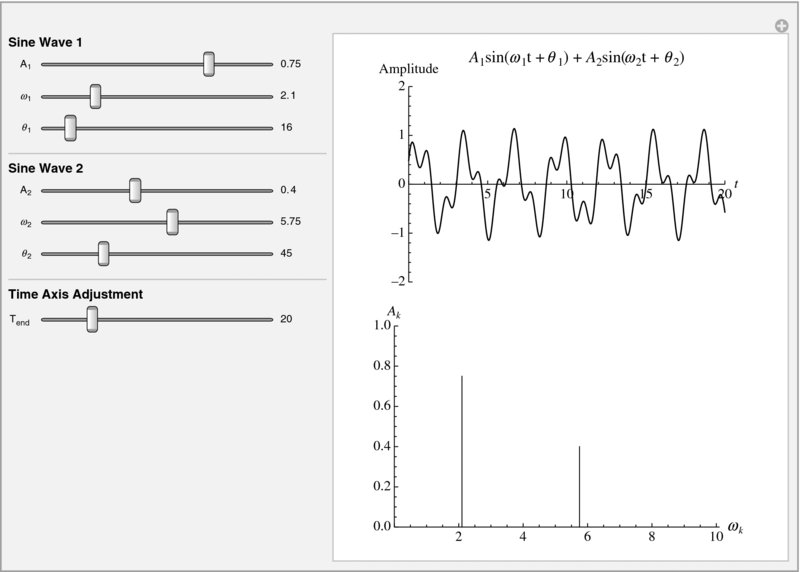
Figure 7.2 Initial interactive display created by Manipulate for Example 7.2
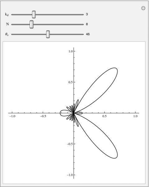
Figure 7.3 Initial interactive display created by Manipulate for the normalized array factor of a steerable array in Example 7.3
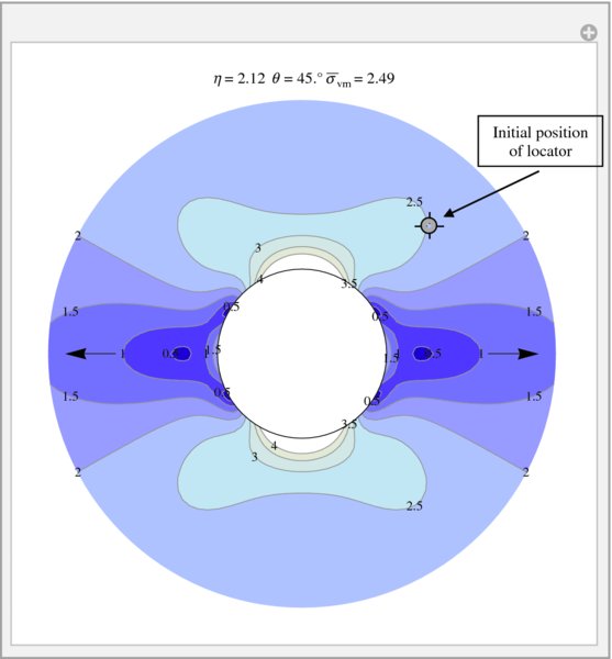
Figure 7.4 Initial interactive display created by Manipulate for obtaining the value of the von Mises stress at any location (η, θ) exterior to the hole, as described in Example 7.4
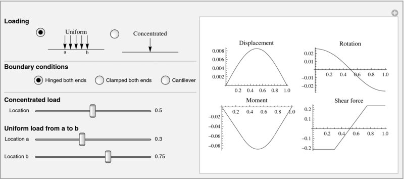
Figure 7.5 Initial interactive display created by Manipulate for obtaining the values that are proportional to the displacement, rotation, moment, and shear force in a beam for two types of loading and their respective locations, and its boundary conditions
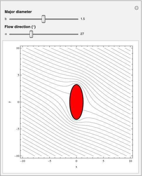
Figure 7.6 Initial interactive display created by Manipulate for obtaining the streamlines of flow around an ellipse for various elliptical shapes and flow directions

Figure 7.7 Four-bar linkage

Figure 7.8 Initial configuration of the interactive display created by Manipulate for animating the motion of a four-bar linkage
References
- G. Currie, Fundamentals of Fluid Mechanics, 2nd edn, McGraw-Hill, Inc., New York, 1993, p. 98.
- B. Balachandran and E. B. Magrab, Vibrations, 2nd edn, Cengage Learning, Toronto Ontario, 2009, pp. 165–7.
Exercises
- 7.1 One model of machine tool chatter gives that the region of instability can be determined from the following equation [2]

where Q is the quality factor, k1 is the cutting stiffness, K is a penetration rate coefficient, k is the work-piece stiffness, μ is the overlap factor (0 ≤ μ ≤ 1), Ω is the nondimensional work piece rotation speed, and ω is the chatter frequency that is the root of
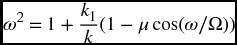
Thus, for a given k1/k, K/k, and μ, a plot of Q versus Ω will display the regions where chatter occurs. The locus of the region where the system is chatter-free is given by

where

Create an interactive graphic that displays the regions of chatter that looks like that shown in Figure 7.9. The ranges for the various parameters are: 0 ≤ μ ≤ 1, 0.07 ≤ k1/ k ≤ 0.08, and 0.0015 ≤ K/k ≤ 0.0035. Use the RegionFunction option to limit Q to the region 0 < Q < 50.

Figure 7.9 Solution to Exercise 7.1
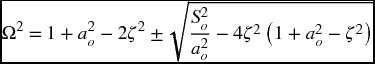
- 7.2 The nondimensional magnitude ao of the amplitude response of the mass of a single degree-of-freedom system with a spring that is proportional to the cube of the displacement of the mass and undergoing harmonic oscillations can be obtained from
where the plus sign displays the right portion of the curve and the minus sign the left portion. The quantity Ω is the nondimensional frequency ratio, So is related to the magnitude of the harmonic input, and ζ is the damping factor. The curve that is midway between the two curves given by Eq. (a) is called the spine and is determined from
The maximum value of ao is obtained from

and the frequency at which it occurs is

In the plotting of the curve corresponding to the plus branch of the curve; that is, the right portion, there is an inflection point. This inflection point is determined numerically by finding the value of ao that causes Ω to be a minimum.
The procedure to plot these curves and display their values is as follows. One selects a value of ao and uses Eq. (a) to determine the corresponding values of Ω for the left and right curves. In a similar fashion, the spines of the curves are determined using Eq. (b). Then the location of the maximum value of ao = amax is computed and, lastly, the inflection point is determined from the right side of Eq. (a).
Create an interactive graphic that does these computations and displays the results as shown in Figure 7.10. Let 0.1 ≤ So ≤ 2 and 0.02 ≤ ao ≤ amax.

Figure 7.10 Solution to Exercise 7.2