7
BASIC ASYMPTOTICS: LARGE SAMPLE THEORY
7.1 INTRODUCTION
In Chapter 6 we described some methods of finding exact distributions of sample statistics and their moments. While these methods are used in some cases such as sampling from a normal population when the sample statistic of interest is ![]() or S2, often either the statistics of interest, say
or S2, often either the statistics of interest, say ![]() , is either too complicated or its exact distribution is not simple to work with. In such cases we are interested in the convergence properties of Tn. We want to know what happens when the sample size is large. What is the limiting distribution of Tn? When the exact distribution of Tn (and its moments) is unknown or too complicated we will often use their asymptotic approximations when n is large.
, is either too complicated or its exact distribution is not simple to work with. In such cases we are interested in the convergence properties of Tn. We want to know what happens when the sample size is large. What is the limiting distribution of Tn? When the exact distribution of Tn (and its moments) is unknown or too complicated we will often use their asymptotic approximations when n is large.
In this chapter, we discuss some basic elements of statistical asymptotics. In Section 7.2 we discuss various modes of convergence of a sequence of random variables. In Sections 7.3 and 7.4 the laws of large numbers are discussed. Section 7.5 deals with limiting moment generating functions and in Section 7.6 we discuss one of the most fundamental theorem of classical statistics called the central limit theorem. In Section 7.7 we consider some statistical applications of these methods.
The reader may find some parts of this chapter a bit difficult on first reading. Such a discussion has been indicated with a†.
7.2 MODES OF CONVERGENCE
In this section we consider several modes of convergence and investigate their interrelationships. We begin with the weakest mode of convergence.
It must be remembered that it is quite possible for a given sequence DFs to converge to a function that is not a DF.
We next give an example to show that weak convergence of distribution functions does not imply the convergence of corresponding PMF’s or PDF’s.
The following result is easy to prove.
In the continuous case we state the following result of Scheffé [100] without proof.
The following result is easy to establish.
A slightly stronger concept of convergence is defined by convergence in probability.
Remark 1. We emphasize that the definition says nothing about the convergence of the RVs Xn to the RV X in the sense in which it is understood in real analysis. Thus ![]() does not imply that, given
does not imply that, given ![]() , we can find an N such that
, we can find an N such that ![]() . Definition 2 speaks only of the convergence of the sequence of probabilities
. Definition 2 speaks only of the convergence of the sequence of probabilities ![]() to 0.
to 0.
The following statements can be verified.
 .
. , for
, for  , and it follows that
  for every
  .
. as
as  , for
, for

 .
. .
. .
. , for
, for

 , for
and each of the three terms on the right goes to 0 as
, for
and each of the three terms on the right goes to 0 as
 .
. .
. and Y an
  .
.
Note that Y is an RV so that, given
 , there exists a
  such that
  . Thus
 , for
The result now follows on multiplication, using result 10. It also follows that
, for
The result now follows on multiplication, using result 10. It also follows that
 .
.
We remark that a more general result than Theorem 4 is true and state it without proof (see Rao [88, p. 124]): ![]() and g continuous on
and g continuous on ![]() .
.
The following two theorems explain the relationship between weak convergence and convergence in probability.
Remark 2. We emphasize that we cannot improve the above result by replacing k by an RV, that is, ![]() in general does not imply
in general does not imply ![]() , for let X, X1, X2… be identically distributed RVs, and let the joint distribution of (Xn, X) be as follows:
, for let X, X1, X2… be identically distributed RVs, and let the joint distribution of (Xn, X) be as follows:

Clearly, ![]() . But
. But

Hence, ![]() , but
, but ![]() .
.
Remark 3. Example 3 shows that ![]() does not imply
does not imply ![]() for any
for any ![]() , k integral.
, k integral.
We get, in addition, that ![]() implies
implies ![]() .
.
Proof. The proof is left to the reader.
As a simple consequence of Theorem 8 and its corollary we see that ![]() together imply
together imply ![]() .
.
Remark 4. Clearly the converse to Theorem 10 cannot hold, since ![]() does not imply
does not imply ![]() .
.
Remark 5. In view of Theorem 9, it follows that ![]() for
for ![]() .
.
The following result elucidates Definition 4.
Remark 6. Thus ![]() means that, for
means that, for ![]() arbitrary, we can find an n0 such that
arbitrary, we can find an n0 such that

Indeed, we can write, equivalently, that

That the converse of Theorem 12 does not hold is shown in the following example.
Remark 7. In Theorem 7.4.3 we prove a result which is sometimes useful in proving a.s. convergence of a sequence of RVs.
Since ![]() is arbitrary and x is a continuity point of
is arbitrary and x is a continuity point of ![]() , we get the result by letting
, we get the result by letting ![]() .
.
Later on we will see that the condition that the Xi’s be ![]() (0, 1) is not needed. All we need is that
(0, 1) is not needed. All we need is that ![]() .
.
PROBLEMS 7.2
- Let X1, X2,… be a sequence of RVs with corresponding DFs given by
 if
if  . Does Fn converge to a DF?
 - Let X1, X2… be iid
 (0, 1) RVs. Consider the sequence of RVs
  , where
  . Let Fn be the DF of
  ., Find
  . Is this limit a DF?
 - Let X1, X2,… be iid U(0, θ) RVs. Let
 , and consider the sequence
  . Does Yn converge in distribution to some RV Y? If so, find the DF of RV Y.
 - Let X1, X2 be iid RVs with common absolutely continuous DF F. Let
 , and consider the sequence of
 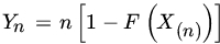 . Find the limiting DF of Yn.
- Let X1, X2,… be a sequence of iid RVs with common PDF
 . Write
  .
.
- Show that
 .
. - Show that
 .
.
- Show that
- Let X1, X2,… be iid U[0, θ] RVs. Show that
 .
. - Let {Xn} be a sequence of RVs such that
 . Let an be a sequence of positive constants such that
  . Show that
  .
. - Let {Xn} be a sequence of RVs such that
 for all n and some constant
  . Suppose that
  . Show that
  for any
  .
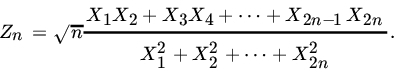
. - Let X1, X2,…, X2n be iid (0, 1) RVs. Define

Find the limiting distribution of Zn.
- Let {Xn} be a sequence of geometric RVs with parameter
 . Also, let
  . Show that
  as
as 
(Prochaska [82]).
- Let Xn be a sequence of RVs such that
 , and let cn be a sequence of real numbers such that
  as
as  . Show that
  .
. - Does convergence almost surely imply convergence of moments?
- Let X1, X2,… be a sequence of iid RVs with common DF F, and write
 .
.
- For
 ,
,  . Find the limiting distribution of
  . Also, find the PDF corresponding to the limiting DF and compute its moments
 - If F satisfies
find the limiting DF of

 and compute the corresponding PDF and the MGF.
 - If Xi is bounded above by x0 with probability 1, and for some
 find the limiting distribution of
 , the corresponding PDF, and the moments of the limiting distribution.
(The above remarkable result, due to Gnedenko [36], exhausts all limiting distributions of X(n) with suitable norming and centering.)
- For
- Let {Fn} be a sequence of DFs that converges weakly to a DF F which is continuous everywhere. Show that Fn(x) converges to F(x) uniformly.
- Prove Theorem 1.
- Prove Theorem 6.
- Prove Theorem 13.
- Prove Corollary 1 to Theorem 8.
- Let V be the class of all random variables defined on a probability space with finite expectations, and for
 define
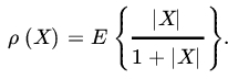
Show the following:
 .
. is a distance function on V (assuming that we identify RVs that are a.s. equal).
 .
.
- For the following sequences of RVs {Xn}, investigate convergence in probability and convergence in rth mean.
 .
. .
.
7.3 WEAK LAW OF LARGE NUMBERS
Let {Xn} be a sequence of RVs. Write, ![]() . In this section we answer the following question in the affirmative: Do there exist sequences of constants An and
. In this section we answer the following question in the affirmative: Do there exist sequences of constants An and ![]() , such that the sequence of RVs
, such that the sequence of RVs ![]() converges in probability to 0 as
converges in probability to 0 as ![]() ?
?
Remark 1. Since condition (1) applies not to the individual variables but to their sum, Theorem 2 is of limited use. We note, however, that all weak laws of large numbers obtained as corollaries to Theorem 1 follow easily from Theorem 2 (Problem 6).
Let X1, X2,… be an arbitrary sequence of RVs, and let ![]() . Let us truncate each Xi at
. Let us truncate each Xi at ![]() , that is, let
, that is, let

Write

Inequality (6) yields the following important theorem.
We emphasize that in Theorem 3 we require only that ![]() ; nothing is said about the variance. Theorem 3 is due to Khintchine.
; nothing is said about the variance. Theorem 3 is due to Khintchine.
PROBLEMS 7.3
- Let X1, X2,… be a sequence of iid RVs with common uniform distribution on [0, 1]. Also, let
 be the geometric mean of X1, X2,…,Xn,
  . Show that
  , where c is some constant. Find c.
 - Let X1, X2,… be iid RVs with finite second moment. Let

Show that
 .
. - Let X1, X2,… be a sequence of iid RVs with
 and
and  . Let
. Let  . Does the sequence Sk obey the WLLN in the sense of Definition 1? If so, find the centering and the norming constants.
Yes;

- Let {Xn} be a sequence of RVs for which
 for all n and
  . Show that the WLLN holds.
 - For the following sequences of independent RVs does the WLLN hold?
 .
. .
. .
. .
. .
.
- Let X1, X2,… be a sequence of independent RVs such that
 for
for  , and
, and 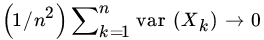 as
as  . Prove the WLLN, using Theorem 2.
 - Let Xn be a sequence of RVs with common finite variance σ2. Suppose that the correlation coefficient between Xi and Xj is < 0 for all
 . Show that the WLLN holds for the sequence {Xn}.
 - Let {Xn} be a sequence of RVs such that Xk is independent of Xj for
 or
or  . If
. If  for all k, where C is some constant, the WLLN holds for {Xk}.
 - For any sequence of RVs {Xn} show that

- Let X1, X2,… be iid
 (1, 0) RVs. Use Theorem 2 to show that the weak law of large numbers does not hold. That is, show that

- Let {Xn} be a sequence of iid RVs with
 . Let
. Let  . Suppose {an} is a sequence of constants such that
  . Show that
 as
as  and (b)
  .
.
7.4 STRONG LAW OF LARGE NUMBERS†
In this section we obtain a stronger form of the law of large numbers discussed in Section 7.3. Let X1, X2,… be a sequence of RVs defined on some probability space (Ω, ![]() , P).
, P).
We will obtain sufficient conditions for a sequence {Xn} to obey the SLLN. In what follows, we will be interested mainly in the case ![]() . Indeed, when we speak of the SLLN we will assume that we are speaking of the norming constants
. Indeed, when we speak of the SLLN we will assume that we are speaking of the norming constants ![]() , unless specified otherwise.
, unless specified otherwise.
We start with the Borel-Cantelli lemma. Let {Aj} be any sequence of events in ![]() . We recall that
. We recall that
We will write ![]() . Note that A is the event that infinitely many of the An occur. We will sometimes write
. Note that A is the event that infinitely many of the An occur. We will sometimes write
where “i.o.” stands for “infinitely often.” In view of Theorem 7.2.11 and Remark 7.2.6 we have ![]() if and only if
if and only if ![]() for all
for all ![]() .
.
We next prove some important lemmas that we will need subsequently.
As a corollary we get a version of the SLLN for nonidentically distributed RVs which subsumes Theorem 2.
Remark 1. Kolmogorov’s SLLN is much stronger than Corollaries 1 and 4 to Theorem 4. It states that if {Xn} is a sequence of iid RVs then
and then ![]() . The proof requires more work and will not be given here. We refer the reader to Billingsley [6], Chung [15], Feller [26], or Laha and Rohatgi [58].
. The proof requires more work and will not be given here. We refer the reader to Billingsley [6], Chung [15], Feller [26], or Laha and Rohatgi [58].
PROBLEMS 7.4
- For the following sequences of independent RVs does the SLLN hold?
 .
. .
. .
.
- Let X1, X2,… be a sequence of independent RVs with
 . Show that

Does the converse also hold?
- For what values of α does the SLLN hold for the sequence

- Let
 be a sequence of real numbers such that
  . Show that there exists a sequence of independent RVs {Xk} with
  , such that
  does not converge to 0 almost surely.
[Hint: Let
 , and
, and  . Apply the Borel-Cantelli lemma to
  .]
.] - Let Xn be a sequence of iid RVs with
 . Show that, for every positive number
  and
and  .
. - Construct an example to show that the converse of Theorem 1(a) does not hold.
- Investigate a.s. convergence of {Xn} to 0 in each case.
 .
. .
.
(Xn’s are independent in each case.)
7.5 LIMITING MOMENT GENERATING FUNCTIONS
Let X1,X2,… be a sequence of RVs. Let Fn be the DF of ![]() , and suppose that the MGF Mn(t) of Fn exists. What happens to Mn(t) as
, and suppose that the MGF Mn(t) of Fn exists. What happens to Mn(t) as ![]() ? If it converges, does it always converge to an MGF?
? If it converges, does it always converge to an MGF?
Next suppose that Xn has MGF Mn and ![]() , where X is an RV with MGF M. Does
, where X is an RV with MGF M. Does ![]() ? The answer to this question is in the negative.
? The answer to this question is in the negative.
The following result is a weaker version of the continuity theorem due to Lévy and Cramér. We refer the reader to Lukacs [69, p. 47], or Curtiss [19], for details of the proof.
Remark 1. The following notation on orders of magnitude is quite useful. We write ![]() if, given
if, given ![]() , there exists an N such that
, there exists an N such that ![]() for all
for all ![]() and
and ![]() if there exists an N and a constant
if there exists an N and a constant ![]() , such that |xn/rn| for all
, such that |xn/rn| for all ![]() . We write
. We write ![]() to express the fact that xn is bounded for large n, and
to express the fact that xn is bounded for large n, and ![]() to mean that
to mean that ![]() as
as ![]() .
.
This notation is extended to RVs in an obvious manner. Thus ![]() if, for every
if, for every ![]() and
and ![]() , there exists an N such that
, there exists an N such that ![]() for
for ![]() , and
, and ![]() if, for
if, for ![]() , there exists a
, there exists a ![]() and an N such that
and an N such that ![]() . We write
. We write ![]() to mean
to mean ![]() . This notation can be easily extended to the case where rn itself is an RV.
. This notation can be easily extended to the case where rn itself is an RV.
The following lemma is quite useful in applications of Theorem 1.
For more examples see Section 7.6.
Remark 2. As pointed out earlier working with MGFs has the disadvantage that the existence of MGFs is a very strong condition. Working with CFs which always exist, on the other hand, permits a much wider application of the continuity theorem. Let ϕn be the CF of Fn. Then ![]() if and only if
if and only if ![]() as
as ![]() on
on ![]() , where ϕ is continuous at
, where ϕ is continuous at ![]() . In this case ϕ, the limit function, is the CF of the limit DF F.
. In this case ϕ, the limit function, is the CF of the limit DF F.
PROBLEMS 7.5
- Let
 . Show that

here
 .
. - Let
 . Show that
  as
as  , in such a way that
  , where
  .
. - Let X1, X2… be independent RVs with PMF given by
 . Let
. Let  . Show that
  , where
  .
. - Let {Xn} be a sequence of RVs with
 where
where  is a constant (independent of n). Find the limiting distribution of Xn/n.
 - Let
 . Find the limiting distribution of Xn/n2.
- Let X1, X2,…, Xn be jointly normal with
 for all i and
  . What is the limiting distribution of n— 1Sn, where
7.6 CENTRAL LIMIT THEOREM
Let X1, X2,… be a sequence of RVs, and let ![]() . In Sections 7.3 and 7.4 we investigated the convergence of the sequence of RVs
. In Sections 7.3 and 7.4 we investigated the convergence of the sequence of RVs ![]() to the degenerate RV. In this section we examine the convergence of
to the degenerate RV. In this section we examine the convergence of ![]() to a nondegenerate RV. Suppose that, for a suitable choice of constants An and
to a nondegenerate RV. Suppose that, for a suitable choice of constants An and ![]() , the RVs
, the RVs ![]() . What are the properties of this limit RV Y? The question as posed is far too general and is not of much interest unless the RVs Xi are suitably restricted. For example, if we take X1 with DF F and X2, X3,… to be 0 with probability 1, choosing
. What are the properties of this limit RV Y? The question as posed is far too general and is not of much interest unless the RVs Xi are suitably restricted. For example, if we take X1 with DF F and X2, X3,… to be 0 with probability 1, choosing ![]() and
and ![]() leads to F as the limit DF.
leads to F as the limit DF.
We recall (Example 7.5.6) that, if X1, X2,…, Xn are iid RVs with common law ![]() (1, 0), then
(1, 0), then ![]() is also
is also ![]() (1,0). Again, if X1, X2,…, Xn are iid
(1,0). Again, if X1, X2,…, Xn are iid ![]() (0, 1) RVs then
(0, 1) RVs then ![]() is also
is also ![]() (0, 1) (Corollary 2 to Theorem 5.3.22). We note thus that for certain sequences of RVs there exist sequences An and
(0, 1) (Corollary 2 to Theorem 5.3.22). We note thus that for certain sequences of RVs there exist sequences An and ![]() , such that
, such that ![]() . In the Cauchy case
. In the Cauchy case ![]() ,
, ![]() , and in the normal case
, and in the normal case ![]() . Moreover, we see that Cauchy and normal distributions appear as limiting distributions—in these two cases, because of the reproductive nature of the distributions. Cauchy and normal distributions are examples of stable distributions.
. Moreover, we see that Cauchy and normal distributions appear as limiting distributions—in these two cases, because of the reproductive nature of the distributions. Cauchy and normal distributions are examples of stable distributions.
Let X1, X2,… be iid RVs with common DF F. We remark without proof (see Loève [66, p. 339]) that only stable distributions occur as limits. To make this statement more precise we make the following definition.
In view of the statement after Definition 1, we see that only stable distributions possess domains of attraction. From Definition 1 we also note that each stable law belongs to its own domain of attraction. The study of stable distributions is beyond the scope of this book. We shall restrict ourselves to seeking conditions under which the limit law V is the normal distribution. The importance of the normal distribution in statistics is due largely to the fact that a wide class of distributions F belongs to the domain of attraction of the normal law. Let us consider some examples.
These examples suggest that if we take iid RVs with finite variance and take ![]() , then
, then ![]() , where Z is
, where Z is ![]() (0, 1). This is the central limit result, which we now prove. The reader should note that in both Examples 1 and 2 we used more than just the existence of E|X|2. Indeed, the MGF exists and hence moments of all order exist. The existence of MGF is not a necessary condition.
(0, 1). This is the central limit result, which we now prove. The reader should note that in both Examples 1 and 2 we used more than just the existence of E|X|2. Indeed, the MGF exists and hence moments of all order exist. The existence of MGF is not a necessary condition.
Remark 1. In the proof above we could have used the Taylor series expansion of M to arrive at the same result.
Remark 2. Even though we proved Theorem 1 for the case when the MGF of Xn’s exists, we will use the result whenever ![]() . The use of CFs would have provided a complete proof of Theorem 1. Let ϕ be the CF of Xn. Assuming again, without loss of generality, that
. The use of CFs would have provided a complete proof of Theorem 1. Let ϕ be the CF of Xn. Assuming again, without loss of generality, that ![]() , we can write
, we can write
Thus the CF of ![]() is
is

which converges to ![]() which is the CF of a
which is the CF of a ![]() (0, 1) RV. The devil is in the details of the proof.
(0, 1) RV. The devil is in the details of the proof.
The following converse to Theorem 1 holds.
For nonidentically distributed RVs we state, without proof, the following result due to Lindeberg.
Feller [24] has shown that condition (2) is necessary as well in the following sense. For independent RVs {Xk} for which (3) holds and

(2) holds for every ![]() .
.
If ![]() , then
, then ![]() , say, as
, say, as ![]() . For fixed k, we can find εk such that
. For fixed k, we can find εk such that ![]() and then
and then ![]() . For
. For ![]() , we have
, we have

so that the Lindeberg condition does not hold. Indeed, if X1, X2,…. are independent RVs such that there exists a constant A with ![]() for all n, the Lindeberg condition (2) is satisfied if
for all n, the Lindeberg condition (2) is satisfied if ![]() . To see this, suppose that
. To see this, suppose that ![]() . Since the Xk’s are uniformly bounded, so are the RVs Xk–EXk. It follows that for every
. Since the Xk’s are uniformly bounded, so are the RVs Xk–EXk. It follows that for every ![]() we can find an Nε such that, for
we can find an Nε such that, for ![]() . The Lindeberg condition follows immediately. The converse also holds, for, if
. The Lindeberg condition follows immediately. The converse also holds, for, if ![]() and the Lindeberg condition holds, there exists a constant
and the Lindeberg condition holds, there exists a constant ![]() such that
such that ![]() . For any fixed j, we can find an
. For any fixed j, we can find an ![]() such that
such that ![]() . Then, for
. Then, for ![]() ,
,

and the Lindeberg condition does not hold. This contradiction shows that ![]() is also a necessary condition that is, for a sequence of uniformly bounded independent RVs, a necessary and sufficient condition for the central limit theorem to hold is
is also a necessary condition that is, for a sequence of uniformly bounded independent RVs, a necessary and sufficient condition for the central limit theorem to hold is ![]() as
as ![]() .
.
Remark 3. Both the central limit theorem (CLT) and the (weak) law of large numbers (WLLN) hold for a large class of sequences of RVs {Xn}. If the {Xn} are independent uniformly bounded RVs, that is, if ![]() , the WLLN (Theorem 7.3.1) holds; the CLT holds provided that
, the WLLN (Theorem 7.3.1) holds; the CLT holds provided that ![]() (Example 5).
(Example 5).
If the RVs {Xn} are iid, then the CLT is a stronger result than the WLLN in that the former provides an estimate of the probability ![]() . Indeed,
. Indeed,

where Z is ![]() (0, 1), and the law of large number follows. On the other hand, we note that the WLLN does not require the existence of a second moment.
(0, 1), and the law of large number follows. On the other hand, we note that the WLLN does not require the existence of a second moment.
Remark 4. If {Xn} are independent RVs, it is quite possible that the CLT may apply to the Xn’s, but not the WLLN.
We conclude this section with some remarks concerning the application of the CLT. Let X1, X2,… be iid RVs with common mean μ and variance σ2. Let us write

and let ![]() 1,
1, ![]() 2 be two arbitrary real numbers with
2 be two arbitrary real numbers with ![]() . If Fn is the DF of Zn, then
. If Fn is the DF of Zn, then

that is,
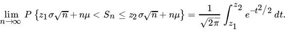
It follows that the RV ![]() is asymptotically normally distributed with mean nμ and variance nσ2. Equivalently, the RV
is asymptotically normally distributed with mean nμ and variance nσ2. Equivalently, the RV ![]() is asymptotically
is asymptotically ![]() . This result is of great importance in statistics.
. This result is of great importance in statistics.
In Fig. 1 we show the distribution of ![]() in sampling from P(λ) and G (1, 1). We have also superimposed, in each case, the graph of the corresponding normal approximation.
in sampling from P(λ) and G (1, 1). We have also superimposed, in each case, the graph of the corresponding normal approximation.


Fig. 1 (a) Distribution of  for Poisson RV with mean 3 and normal approximation and (b) distribution of
  for exponential RV with mean 1 and normal approximation.
How large should n be before we apply approximation (4)? Unfortunately the answer is not simple. Much depends on the underlying distribution, the corresponding speed of convergence, and the accuracy one desires. There is a vast amount of literature on the speed of convergence and error bounds. We will content ourselves with some examples. The reader is referred to Rohatgi [90] for a detailed discussion.
In the discrete case when the underlying distribution is integer-valued, approximation (4) is improved by applying the continuity correction. If X is integer-valued, then for integers x1, x2
which amounts to making the discrete space of values of X continuous by considering intervals of length 1 with midpoints at integers.
Next suppose that ![]() . Then from binomial tables
. Then from binomial tables ![]() . Using normal approximation, without continuity correction
. Using normal approximation, without continuity correction
and with continuity correction
The rule of thumb is to use continuity correction, and use normal approximation whenever ![]() , and use Poisson approximation with
, and use Poisson approximation with ![]() for
for ![]() .
.
PROBLEMS 7.6
- Let {Xn} be a sequence of independent RVs with the following distributions. In each case, does the Lindeberg condition hold?
 .
. .
. .
.- {Xn} is a sequence of independent Poisson RVs with parameter
 , such that
  .
.  .
.
- Let X1, X2,… be iid RVs with mean 0, variance 1, and
 . Find the limiting distribution of
- Let X1, X2,… be iid RVs with mean α and variance σ2, and let Y1,Y2,… be iid RVs with mean
 and variance τ2. Find the limiting distribution of
  , where
  and
and  .
. - Let
 . Use the CLT to find n such that
  . In particular, let
  and
and  . Calculate n, satisfying
  .
. - Let X1, X2,… be a sequence of iid RVs with common mean μ and variance σ2. Also, let
 and
and  . Show that
  where
where  .
. - Let X1, X2,…, X100 be iid RVs with mean 75 and variance 225. Use Chebychev’s inequality to calculate the probability that the sample mean will not differ from the population mean by more than 6. Then use the CLT to calculate the same probability and compare your results.
- Let X1, X2,…,X100 be iid P(λ) RVs, where
 . Let
. Let  . Use the central limit result to evaluate
  and compare your result to the exact probability of the event
  .
. - Let X1, X2,…,X81 be iid RVs with mean 54 and variance 225. Use Chebychev’s inequality to find the possible difference between the sample mean and the population mean with a probability of at least 0.75. Also use the CLT to do the same.
0.0926; 1.92
- Use the CLT applied to a Poisson RV to show that
 for
for  if
if  , and 0 if
  .
. - Let X1,X2,… be a sequence of iid RVs with mean μ and variance σ2, and assume that
 . Write
  . Find the centering and norming constants An and Bn such that
  , where Z is (0, 1).
 - From an urn containing 10 identical balls numbered 0 through 9, n balls are drawn with replacement.
- What does the law of large numbers tell you about the appearance of 0’s in the n drawings?
- How many drawings must be made in order that, with probability at least 0.95, the relative frequency of the occurrence of 0’s will be between 0.09 and 0.11?
- Use the CLT to find the probability that among the n numbers thus chosen the number 5 will appear between
 and
and  times (inclusive) if (i)
  and (ii)
  .
.
- Let X1, X2,…,Xn be iid RVs with
 and
and  . Let
. Let  , and for any positive real number ε let
  . Show that

[Hint: Use (5.3.61.]
7.7 LARGE SAMPLE THEORY
In many applications of probability one needs the distribution of a statistic or some function of it. The methods of Section 7.3 when applicable lead to the exact distribution of the statistic under consideration. If not, it may be sufficient to approximate this distribution provided the sample size is large enough.
Let {Xn} be a sequence of RVs which converges in law to N(μ, σ2). Then ![]() converges in law to N(0, 1), and conversely. We will say alternatively and equivalently that {Xn} is asymptotically normal with mean μ and variance σ2 More generally, we say that Xn is asymptotically normal with “mean” μn and “variance”.
converges in law to N(0, 1), and conversely. We will say alternatively and equivalently that {Xn} is asymptotically normal with mean μ and variance σ2 More generally, we say that Xn is asymptotically normal with “mean” μn and “variance”. ![]() , and write Xn is AN
, and write Xn is AN ![]() , if
, if ![]() and as
and as ![]() .
.
Here μn is not necessarily the mean of Xn and. ![]() , not necessarily its variance. In this case we can approximate, for sufficiently large n,
, not necessarily its variance. In this case we can approximate, for sufficiently large n, ![]() by
by  , where Z is
 ![]() (0, 1).
(0, 1).
The most common method to show that Xn is ![]() is the central limit theorem of Section 6. Thus, according to Theorem 7.6.1
is the central limit theorem of Section 6. Thus, according to Theorem 7.6.1 ![]() as
as ![]() , where
, where ![]() is the sample mean of n iid RVs with mean μ and variance σ2. The same result applies to kth sample moment, provided
is the sample mean of n iid RVs with mean μ and variance σ2. The same result applies to kth sample moment, provided ![]() . Thus
. Thus

In many large sample approximations an application of the CLT along with Slutsky’s theorem suffices.
Often we need to approximate the distribution of g(Yn) given that Yn is AN(μ, σ2).
Remark 1. Suppose in Theorem 1 is differentiable k times, ![]() , at
, at ![]() and
and ![]() for
for ![]() . Then a similar argument using Taylor’s theorem shows that
. Then a similar argument using Taylor’s theorem shows that

Where Z is a ![]() (0, 1) RV. Thus in Example 2, when
(0, 1) RV. Thus in Example 2, when ![]() . It follows that
. It follows that
Since ![]() .
.
Remark 2. Theorem 1 can be extended to the multivariate case but we will not pursue the development. We refer the reader to Ferguson [29] or Serfling [102].
Remark 3. In general the asymptotic variance ![]() of g(Yn) will depend on the parameter μ. In problems of inference it will often be desirable to use transformation g such that the approximate variance var g(Yn) is free of the parameter. Such transformations are called variance stabilizing transformations. Let us write
of g(Yn) will depend on the parameter μ. In problems of inference it will often be desirable to use transformation g such that the approximate variance var g(Yn) is free of the parameter. Such transformations are called variance stabilizing transformations. Let us write ![]() . Then finding a g such that var g(Yn) is free of μ is equivalent to finding a g such that
. Then finding a g such that var g(Yn) is free of μ is equivalent to finding a g such that
for all μ, where c is a constant independent of μ. It follows that

Remark 4. In Section 6.3 we computed exact moments of some statistics in terms of population parameters. Approximations for moments of ![]() can also be obtained from series expansions of g. Suppose g is twice differentiable at
can also be obtained from series expansions of g. Suppose g is twice differentiable at ![]() . Then
. Then
and
by dropping remainder terms. The case of most interest is to approximate ![]() and
and ![]() . In this case, under suitable conditions, one can show that
. In this case, under suitable conditions, one can show that

and

where ![]() and
and ![]() .
.
In Example 2, when Xi’s are iid b(1, p), and ![]() so that
so that

and

In this case we can compute ![]() and
and ![]() exactly. We have
exactly. We have

so that (8) is exact. Also since ![]() , using Theorem 6.3.4 we have
, using Theorem 6.3.4 we have

Thus the error in approximation (9) is

Remark 5. Approximations (6) through (9) do not assert the existence of ![]() or
or ![]() , or var g(X) or
, or var g(X) or ![]() .
.
Remark 6. It is possible to extend (6) through (9) to two (or more) variables by using Taylor series expansion in two (or more) variables.
Finally, we state the following result which gives the asymptotic distribution of the rth order statistic, ![]() , in sampling from a population with an absolutely continuous DF F with PDF f. For a proof see Problem 4.
, in sampling from a population with an absolutely continuous DF F with PDF f. For a proof see Problem 4.
Remark 7. The sample quantile of order p, Zp, is

where ![]() is the corresponding population quantile, and f is the PDF of the population distribution function. It also follows that
is the corresponding population quantile, and f is the PDF of the population distribution function. It also follows that ![]() .
.
PROBLEMS 7.7
- In sampling from a distribution with mean μ and variance σ2 find theasymptotic distribution of
 ,
, ,
, ,
,
both when
 and when
  .
. - Let
 . Then
  . Find a transformation g such that
  has an asymptotic (0, c) distribution for large μ where c is a suitable constant.
 - Let X1,X2,…,Xn be a sample from an absolutely continuous DF F with PDF f. Show that

[Hint:Let Y be an RV with mean μ and ϕ be a Borel function such that E ϕ (Y) exists. Expand ϕ (Y) about the point μ by a Taylor series expansion, and use the fact that
 .]
.] - Prove Theorem 2. [Hint: For any real μ and
 compute the PDF of
  and show that the standardized
  , is asymptotically (0, 1) under the conditions of the theorem.]
 - Let
 . Then
  is AN(0, 1) and X/n is
  . Find a transformation g such that the distribution of
  is AN(0, c).
 - Suppose X is G(1, θ). Find g such that
 is AN(0, c).
 - Let X1,X2,…,Xn be iid RVs with
 . Let
. Let  and
and  :
:
- Show, using the CLT for iid RVs, that
 .
. - Find a transformation g such that g(S2) has an asymptotic distribution which depends on β2 alone but not on σ2.
- Show, using the CLT for iid RVs, that