6
SAMPLE STATISTICS AND THEIR DISTRIBUTIONS
6.1 INTRODUCTION
In the preceding chapters we discussed fundamental ideas and techniques of probability theory. In this development we created a mathematical model of a random experiment by associating with it a sample space in which random events correspond to sets of a certain σ-field. The notion of probability defined on this σ-field corresponds to the notion of uncertainty in the outcome on any performance of the random experiment.
In this chapter we begin the study of some problems of mathematical statistics. The methods of probability theory learned in preceding chapters will be used extensively in this study.
Suppose that we seek information about some numerical characteristics of a collection of elements called a population. For reasons of time or cost we may not wish or be able to study each individual element of the population. Our object is to draw conclusions about the unknown population characteristics on the basis of information on some characteristics of a suitably selected sample. Formally, let X be a random variable which describes the population under investigation, and let F be the DF of X. There are two possibilities. Either X has a DF Fθ with a known functional form (except perhaps for the parameter θ, which may be a vector) or X has a DF F about which we know nothing (except perhaps that F is, say, absolutely continuous). In the former case let Θ be the set of possible values of the unknown parameter θ. Then the job of a statistician is to decide, on the basis of a suitably selected sample, which member or members of the family {Fθ, θ ∈ Θ} can represent the DF of X. Problems of this type are called problems of parametric statistical inference and will be the subject of investigation in Chapters 8 through 12. The case in which nothing is known about the functional form of the DF F of X is clearly much more difficult. Inference problems of this type fall into the domain of nonparametric statistics and will be discussed in Chapter 13.
To be sure, the scope of statistical methods is much wider than the statistical inference problems discussed in this book. Statisticians, for example, deal with problems of planning and designing experiments, of collecting information, and of deciding how best the collected information should be used. However, here we concern ourselves only with the best methods of making inferences about probability distributions.
In Section 6.2 of this chapter we introduce the notions of (simple) random sample and sample statistics. In Section 6.3 we study sample moments and their exact distributions. In Section 6.4 we consider some important distributions that arise in sampling from a normal population. Sections 6.5 and 6.6 are devoted to the study of sampling from univariate and bivariate normal distributions.
6.2 RANDOM SAMPLING
Consider a statistical experiment that culminates in outcomes x, which are the values assumed by an RV X. Let F be the DF of X. In practice, F will not be completely known, that is, one or more parameters associated with F will be unknown. The job of a statistician is to estimate these unknown parameters or to test the validity of certain statements about them. She can obtain n independent observations on X. This means that she observes n values x1, x2,…,xn assumed by the RV X. Each xi can be regarded as the value assumed by an RV ![]() , where X1, X2,…,Xn are independent RVs with common DF F. The observed values (x1, x2,…,xn) are then values assumed by (X1, X2,…,Xn). The set {X1, X2,…,Xn} is then a sample of size n taken from a population distribution F. The set of n values x1, x2,…,xn is called a realization of the sample. Note that the possible values of the RV (X1, X2,…,Xn) can be regarded as points in
, where X1, X2,…,Xn are independent RVs with common DF F. The observed values (x1, x2,…,xn) are then values assumed by (X1, X2,…,Xn). The set {X1, X2,…,Xn} is then a sample of size n taken from a population distribution F. The set of n values x1, x2,…,xn is called a realization of the sample. Note that the possible values of the RV (X1, X2,…,Xn) can be regarded as points in ![]() n, which may be called the sample space. In practice one observes not x1, x2,…,xn but some function f(x1, x2,…,xn). Then f(x1, x2,…,xn) are values assumed by the RV f(X1, X2,…,Xn).
n, which may be called the sample space. In practice one observes not x1, x2,…,xn but some function f(x1, x2,…,xn). Then f(x1, x2,…,xn) are values assumed by the RV f(X1, X2,…,Xn).
Let us now formalize these concepts.
PROBLEMS 6.2
- Let X be a
 , RV, and consider all possible random samples of size 3 on X. Compute
  and S2 for each of the eight samples, and also compute the PMFs of
  and S2.
- A fair die is rolled. Let X be the face value that turns up, and X1, X2 be two independent observations on X. Compute the PMF of
 .
.
- Let X1, X2,…,Xn be a sample from some population. Show that
unless either all the n observations are equal or exactly
 of the Xj’s are equal.
(Samuelson [99])
- Let x1, x2,…,xn be real numbers, and let
 . Show that for any set of real numbers a1, a2,…,an such that
  the following inequality holds:
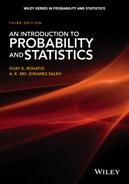
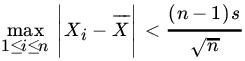
- For any set of real numbers x1, x2,…,xn show that the fraction of x1, x2,…,xn included in the interval
 for
for  is at least
  . Here
  is the mean and s the standard deviation of x's.
6.3 SAMPLE CHARACTERISTICS AND THEIR DISTRIBUTIONS
Let X1, X2,…,Xn be a sample from a population DF F. In this section we consider some commonly used sample characteristics and their distributions.

Fig. 1 Empirical DF for data of Example 1.
Next we consider the moments of sample characteristics. In the following we write ![]() and
and ![]() for the kth-order population moments. Wherever we use mk (or μk), it will be assumed to exist. Also, σ2 represents the population variance.
for the kth-order population moments. Wherever we use mk (or μk), it will be assumed to exist. Also, σ2 represents the population variance.
We next turn our attention to the distributions of sample characteristics. Several possibilities exist. If the exact sampling distribution is required, the method of transformation described in Section 4.4 can be used. Sometimes the technique of MGF or CF can be applied. Thus, if X1, X2,…,Xn is a random sample from a population distribution for which the MGF exists, the MGF of the sample mean ![]() is given by
is given by

where M is the MGF of the population distribution. If ![]() has one of the known forms, it is possible to write the PDF of
has one of the known forms, it is possible to write the PDF of ![]() . Although this method has the obvious drawback that it applies only to distributions for which all moments exist, we will see in Section 6.5 its effectiveness in the important case of sampling from a normal population where this condition is satisfied. An analog of (27) holds for CFs without any condition on existence of moments. Indeed,
. Although this method has the obvious drawback that it applies only to distributions for which all moments exist, we will see in Section 6.5 its effectiveness in the important case of sampling from a normal population where this condition is satisfied. An analog of (27) holds for CFs without any condition on existence of moments. Indeed,

where ϕ is the CF of Xj.
If ![]() , then
, then ![]() , and
, and ![]() with probabilities
with probabilities ![]() , and
, and ![]() , respectively.
, respectively.
We have already considered the distribution of the sample quantiles in Section 4.7 and the distribution of range ![]() in Example 4.7.4. It can be shown, without much difficulty, that the distribution of the sample median is given by
in Example 4.7.4. It can be shown, without much difficulty, that the distribution of the sample median is given by

where F and f are the population DF and PDF, respectively. If ![]() and the median is taken as the average of X(m) and
and the median is taken as the average of X(m) and ![]() , then
, then


Fig. 2  .
.
The method of MGF (or CF) introduced in this section is particularly effective in computing distributions of commonly used statistics in sampling from a univariate or bivariate normal distribution as we shall see in the next two sections. However, when sampling from nonnormal populations these methods may not be very fruitful in determining the exact distribution of the statistic under consideration. Often the statistic itself may be too intractable. Then we have some of other alternatives at our disposal. One may be able to use the asymptotic distribution of the statistic or one may resort to simulation methods. In Chapter 7 we study some of these procedures.
PROBLEMS 6.3
- Let X1, X2,…,Xn be random sample from a DF F, and let
 be the sample distribution function. Find
  for fixed real numbers x, y.
 - Let
 be the empirical DF of a random sample from DF F. Show that
- For the data of Example 6.2.2 compute the sample distribution function.
-
- Show that the sample correlation coefficient R satisfies
 with equality if and only if all sample points lie on a straight line.
 - If we write
 and
and  , what is the sample correlation coefficient between the U’s and the V’s?
- Show that the sample correlation coefficient R satisfies
-
- A sample of size 2 is taken from the PDF
 , and = 0 otherwise.
Find
 .
. - A sample of size 2 is taken from b(1, p):
- Find
 .
. - Find
 .
.
- Find
- A sample of size 2 is taken from the PDF
- Let X1, X2,…,Xn be a random sample from
 (μ, σ2) Compute the first four sample moments of
  about the origin and about the mean. Also compute the first four sample moments of S2 about the mean.
 - Derive the PDF of the median given in (29) and (30).
- Let U(1), U(2),…,U(n) be the order statistic of a sample size n from U(0, 1). Compute
 for any
  and integer
  . In particular, show that
Show also that the correlation coefficient between U(r) and U(s) for
 is given by
 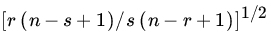 .
. - Let X1, X2,…,Xn be n independent observations on X. Find the sampling distribution of
 , the sample mean, if (a)
  , (b)
, (b)  , and (c)
  .
. - Let X1, X2,…,Xn be a random sample from G(α, β). Let us write
 ..
..- Compute the first four moments of Yn, and compare them with the first four moments of the standard normal distribution.
- Compute the coefficients of skewness α3 and of kurtosis α4 for the RVs Yn. (For definitions of α3, α4 see Problem 3.2.10.)
- Let X1, X2,…,Xn be a random sample from U[0, 1]. Also let
 . Repeat Problem 10 for the sequence Zn.
 - Let X1, X2,…,Xn be a random sample from P(λ). Find var(S2), and compare it with
 . Note that
  . [Hint: Use Problem 3.2.9.]
 - Prove (24) and (25).
- Multiple RVs X1, X2,…,Xn are exchangeable if the n! permutations
 have the same n-dimensional distribution. Consider the special case when X’s are two dimensional. Find an analog of Theorem 6 for exchangeable bivariate RVs (X1,Y1),(X2,Y2),…,(Xn,Yn).
 - Let X1, X2,…,Xn be a random sample from a distribution with finite third moment. Show that
 .
.
6.4 CHI-SQUARE, t-, AND F-DISTRIBUTIONS: EXACT SAMPLING DISTRIBUTIONS
In this section we investigate certain distributions that arise in sampling from a normal population. Let X1, X2,…,Xn be a sample from ![]() (μ,σ2). Then we know that
(μ,σ2). Then we know that ![]() . Also,
. Also, ![]() is
is ![]() (1). We will determine the distribution of S2 in the next section. Here we mainly define chi-square, t-, and F-distributions and study their properties. Their importance will become evident in the next section and later in the testing of statistical hypotheses (Chapter 10).
(1). We will determine the distribution of S2 in the next section. Here we mainly define chi-square, t-, and F-distributions and study their properties. Their importance will become evident in the next section and later in the testing of statistical hypotheses (Chapter 10).
The first distribution of interest is the chi-square distribution, defined in Chapter 5 as a special case of the gamma distribution. Let ![]() be an integer. Then G(n/2, 2) is a
be an integer. Then G(n/2, 2) is a ![]() (n) RV. In view of Theorem 5.3.29 and Corollary 2 to Theorem 5.3.4, the following result holds.
(n) RV. In view of Theorem 5.3.29 and Corollary 2 to Theorem 5.3.4, the following result holds.
We leave the reader to show (Problem 3) that, if T has a noncentral t-distribution with n d.f. and noncentrality parameter δ, then
and


Fig. 4 F densities.
It is shown in Problem 2 that if F has a noncentral F-distribution with (m,n) d.f. and noncentrality parameter δ,

and

PROBLEMS 6.4
- Let

Show that

- Let
 . Find EX and var(X).
 - Let T be a noncentral t-statistic with n d.f. and noncentrality parameter δ. Find ET and var(T).
- Let
 . Then
Deduce that for


- Derive the PDF of an F-statistic with (m,n) d.f.
- Show that the square of a noncentral t-statistic is a noncentral F-statistic.
- A sample of size 16 showed a variance of 5.76. Find c such that
 , where
  is the sample mean and μ is the population mean. Assume that the sample comes from a normal population.
 - A sample from a normal population produced variance 4.0. Find the size of the sample if the sample mean deviates from the population mean by no more than 2.0 with a probability of at least 0.95.
- Let X1, X2, X3, X4, X5 be a sample from
 . Find
  .
. - Let
 . Find
  .
. - Let
 . The random variable
  is known as Fisher’s Z statistic. Find the PDF of Z.
 - Prove Theorem 1.
- Prove Theorem 2.
- Prove Theorem 3.
- Prove Theorem 4.
-
- Let f1, f2,… be PDFs with corresponding MGFs M1, M2,…, respectively. Let αj
 be constants such that
  . Then
  is a PDF with MGF
  .
. - Write the MGF of a
 (n, δ) RV in (6) as
where
 is the MGF of a
  RV and
  ! is the PMF of a P(δ/2) RV. Conclude that PDF of
  is the weighted sum of PDFs of
  RVs,
RVs,  with Poisson weights and hence
- Let f1, f2,… be PDFs with corresponding MGFs M1, M2,…, respectively. Let αj
6.5 DISTRIBUTION OF  IN SAMPLING FROM A NORMAL POPULATION
Let X1, X2,…,Xn be a sample from ![]() (μ, σ2), and write
(μ, σ2), and write ![]() and
and ![]() . In this section we show that
. In this section we show that ![]() and S2 are independent and derive the distribution of S2. More precisely, we prove the following important result.
and S2 are independent and derive the distribution of S2. More precisely, we prove the following important result.
PROBLEMS 6.5
- Let X1, X2,…,Xn be a random sample from
 (μ, σ2) and
  and S2, respectively, be the sample mean and the sample variance. Let
  , and assume that X1,X2,…,Xn,Xn+1 are independent. Find the sampling distribution of
  .
. - Let X1, X2,…,Xm and Y1, Y2,…,Yn be independent random samples from (μ1, σ2) and (μ2, σ2), respectively. Also, let α, β be two fixed real numbers. If
 denote the corresponding sample means, what is the sampling distribution of
where
 and
and  , respectively, denote the sample variances of the X’s and the Y’s?
 - Let X1, X2,…,Xn be a random sample from (μ, σ2), and k be a positive integer. Find E(S2k). In particular, find E(S2) and var(S2).
- A random sample of 5 is taken from a normal population with mean 2.5 and variance
 .
.- Find the probability that the sample variance lies between 30 and 44.
- Find the probability that the sample mean lies between 1.3 and 3.5, while the sample variance lies between 30 and 44.
- The mean life of a sample of 10 light bulbs was observed to be 1327 hours with a standard deviation of 425 hours. A second sample of 6 bulbs chosen from a different batch showed a mean life of 1215 hours with a standard deviation of 375 hours. If the means of the two batches are assumed to be same, how probable is the observed difference between the two sample means?
- Let
 and
and  be the sample variances from two independent samples of sizes
  and
and  from two populations having the same unknown variance σ2. Find (approximately) the probability that
  .
. - Let X1, X2,…,Xn be a sample from (μ, σ2). By using the Helmert orthogonal transformation defined in Remark 3, show that
 and S2 are independent.
 - Derive the joint PDF of
 and S2 by using the transformation described in Remark 4.
6.6 SAMPLING FROM A BIVARIATE NORMAL DISTRIBUTION
Let (X1, Y1), (X2, Y2),…,(Xn, Yn) be a sample from a bivariate normal population with parameters ![]() . Let us write
. Let us write

and

In this section we show that ![]() is independent of
is independent of ![]() and obtain the distribution of the sample correlation coefficient and regression coefficients (at least in the special case where
and obtain the distribution of the sample correlation coefficient and regression coefficients (at least in the special case where ![]() ).
).
As for the distribution of B, note that the conditional PDF of ![]() , given X1, X2,…,Xn,is
, given X1, X2,…,Xn,is ![]() (0,1), so that the conditional PDF of B, given X1, X2,…,Xn, is
(0,1), so that the conditional PDF of B, given X1, X2,…,Xn, is ![]()
![]() . Let us write
. Let us write ![]() . Then the PDF of RV Λ is that of a
. Then the PDF of RV Λ is that of a ![]() RV. Thus the joint PDF of B and Λ is given by
RV. Thus the joint PDF of B and Λ is given by
where g(b|λ) is ![]() , and h2(λ) is
, and h2(λ) is ![]() . We have
. We have

To complete the proof let us write
where ![]() and
and ![]() . Then
. Then ![]() , and
, and

so that the PDF of R is the same as derived above. Also

where the PDF of B* is given by (22). Relations (22) and (24) are used to find the PDF of B. We leave the reader to carry out these simple details.
Remark 3. In view of (23), namely the invariance of R under translation and (positive) scale changes, we note that for fixed n the sampling distribution of R, under ρ = 0, does not depend on μ1,μ2,σ1, and σ2. In the general case when ρ ≠ 0, one can show that for fixed n the distribution of R depends only on ρ but not on μ1,μ2,σ1, and σ2 (see, for example, Cramér [17], p. 398).
Remark 4. Let us change the variable to

Then

and the PDF of T is given by

which is the PDF of a t-statistic with n-2 d.f. Thus T defined by (25) has a ![]() distribution, provided that
distribution, provided that ![]() . This result facilitates the computation of probabilities under the PDF of R when
. This result facilitates the computation of probabilities under the PDF of R when ![]() .
.
Remark 5. To compute the PDF of ![]() , the so-called sample regression coefficient of X on Y, all we need to do is to interchange σ1and σ2in (7).
, the so-called sample regression coefficient of X on Y, all we need to do is to interchange σ1and σ2in (7).
Remark 6. From (7) we can compute the mean and variance of B. For ![]() , clearly
, clearly
and for ![]() , we can show that
, we can show that

Similarly, we can use (6) to compute the mean and variance of R. We have, for ![]() , under
, under ![]() ,
,
and
PROBLEMS 6.6
- Let (X1, Y1), (X2, Y2),…,(Xn, Yn) be a random sample from a bivariate normal population with
 ,
, ,
, , and
, and  . Let
. Let  denote the corresponding sample means, S12, S22, the corresponding sample variances, and S11, the sample covariance. Write
  .Show that the PDF of R is given by
(Rastogi [89])
[Hint: Let
 and
and  , and observe that the random vector (U,V) is also bivariate normal. In fact, U and V are independent.]
 - Let X and Y be independent normal RVs. A sample of
 observations on (X,Y) produces sample correlation coefficient
  . Find the probability of obtaining a value of R that exceeds the observed value.
 - Let X1, X2 be jointly normally distributed with zero means, unit variances, and correlation coefficient ρ. Let S be a χ2(n) RV that is independent of (X1,X2). Then the joint distribution of
 and
and  is known as a central bivariate t-distribution. Find the joint PDF of (Y1, Y2) and the marginal PDFs of Y1 and Y2, respectively.
 - Let (X1,Y2),…,(Xn,Yn) be a sample from a bivariate normal distribution with parameters
 ,
,  ,
,  , and
, and  , i = 1,2,…,n. Find the distribution of the statistic