
Chapter 6. Big Data Processing Concepts

The need to process large volumes of data is not new. When considering the relationship between a data warehouse and its associated data marts, it becomes clear that partitioning a large dataset into a smaller one can speed up processing. Big Data datasets stored on distributed file systems or within a distributed database are already partitioned into smaller datasets. The key to understanding Big Data processing is the realization that unlike the centralized processing, which occurs within a traditional relational database, Big Data is often processed in parallel in a distributed fashion at the location in which it is stored.
Of course, not all Big Data is batch-processed. Some data possesses the velocity characteristic and arrives in a time-ordered stream. Big Data analytics has answers for this type of processing as well. By leveraging in-memory storage architectures, sense-making can occur to deliver situational awareness. An important principle that constrains streaming Big Data processing is called the Speed, Consistency, and Volume (SCV) principle. It is detailed within this chapter as well.
To further the discussion of Big Data processing, each of the following concepts will be examined in turn:
• parallel data processing
• distributed data processing
• Hadoop
• processing workloads
• cluster
Parallel Data Processing
Parallel data processing involves the simultaneous execution of multiple sub-tasks that collectively comprise a larger task. The goal is to reduce the execution time by dividing a single larger task into multiple smaller tasks that run concurrently.
Although parallel data processing can be achieved through multiple networked machines, it is more typically achieved within the confines of a single machine with multiple processors or cores, as shown in Figure 6.1.

Figure 6.1 A task can be divided into three sub-tasks that are executed in parallel on three different processors within the same machine.
Distributed Data Processing
Distributed data processing is closely related to parallel data processing in that the same principle of “divide-and-conquer” is applied. However, distributed data processing is always achieved through physically separate machines that are networked together as a cluster. In Figure 6.2, a task is divided into three sub-tasks that are then executed on three different machines sharing one physical switch.

Hadoop
Hadoop is an open-source framework for large-scale data storage and data processing that is compatible with commodity hardware. The Hadoop framework has established itself as a de facto industry platform for contemporary Big Data solutions. It can be used as an ETL engine or as an analytics engine for processing large amounts of structured, semi-structured and unstructured data. From an analysis perspective, Hadoop implements the MapReduce processing framework. Figure 6.3 illustrates some of Hadoop’s features.

Processing Workloads
A processing workload in Big Data is defined as the amount and nature of data that is processed within a certain amount of time. Workloads are usually divided into two types:
• batch
• transactional
Batch
Batch processing, also known as offline processing, involves processing data in batches and usually imposes delays, which in turn results in high-latency responses. Batch workloads typically involve large quantities of data with sequential read/writes and comprise of groups of read or write queries.
Queries can be complex and involve multiple joins. OLAP systems commonly process workloads in batches. Strategic BI and analytics are batch-oriented as they are highly read-intensive tasks involving large volumes of data. As shown in Figure 6.4, a batch workload comprises grouped read/writes that have a large data footprint and may contain complex joins and provide high-latency responses.
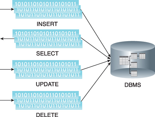
Transactional
Transactional processing is also known as online processing. Transactional workload processing follows an approach whereby data is processed interactively without delay, resulting in low-latency responses. Transaction workloads involve small amounts of data with random reads and writes.
OLTP and operational systems, which are generally write-intensive, fall within this category. Although these workloads contain a mix of read/write queries, they are generally more write-intensive than read-intensive.
Transactional workloads comprise random reads/writes that involve fewer joins than business intelligence and reporting workloads. Given their online nature and operational significance to the enterprise, they require low-latency responses with a smaller data footprint, as shown in Figure 6.5.

Cluster
In the same manner that clusters provide necessary support to create horizontally scalable storage solutions, clusters also provides the mechanism to enable distributed data processing with linear scalability. Since clusters are highly scalable, they provide an ideal environment for Big Data processing as large datasets can be divided into smaller datasets and then processed in parallel in a distributed manner. When leveraging a cluster, Big Data datasets can either be processed in batch mode or realtime mode (Figure 6.6). Ideally, a cluster will be comprised of low-cost commodity nodes that collectively provide increased processing capacity.

Figure 6.6 A cluster can be utilized to support batch processing of bulk data and realtime processing of streaming data.
An additional benefit of clusters is that they provide inherent redundancy and fault tolerance, as they consist of physically separate nodes. Redundancy and fault tolerance allow resilient processing and analysis to occur if a network or node failure occurs. Due to fluctuations in the processing demands placed upon a Big Data environment, leveraging cloud-host infrastructure services, or ready-made analytical environments as the backbone of a cluster, is sensible due to their elasticity and pay-for-use model of utility-based computing.
Processing in Batch Mode
In batch mode, data is processed offline in batches and the response time could vary from minutes to hours. As well, data must be persisted to the disk before it can be processed. Batch mode generally involves processing a range of large datasets, either on their own or joined together, essentially addressing the volume and variety characteristics of Big Data datasets.
The majority of Big Data processing occurs in batch mode. It is relatively simple, easy to set up and low in cost compared to realtime mode. Strategic BI, predictive and prescriptive analytics and ETL operations are commonly batch-oriented.
Batch Processing with MapReduce
MapReduce is a widely used implementation of a batch processing framework. It is highly scalable and reliable and is based on the principle of divide-and-conquer, which provides built-in fault tolerance and redundancy. It divides a big problem into a collection of smaller problems that can each be solved quickly. MapReduce has roots in both distributed and parallel computing. MapReduce is a batch-oriented processing engine (Figure 6.7) used to process large datasets using parallel processing deployed over clusters of commodity hardware.

MapReduce does not require that the input data conform to any particular data model. Therefore, it can be used to process schema-less datasets. A dataset is broken down into multiple smaller parts, and operations are performed on each part independently and in parallel. The results from all operations are then summarized to arrive at the answer. Because of the coordination overhead involved in managing a job, the MapReduce processing engine generally only supports batch workloads as this work is not expected to have low latency. MapReduce is based on Google’s research paper on the subject, published in early 2000.
The MapReduce processing engine works differently compared to the traditional data processing paradigm. Traditionally, data processing requires moving data from the storage node to the processing node that runs the data processing algorithm. This approach works fine for smaller datasets; however, with large datasets, moving data can incur more overhead than the actual processing of the data.
With MapReduce, the data processing algorithm is instead moved to the nodes that store the data. The data processing algorithm executes in parallel on these nodes, thereby eliminating the need to move the data first. This not only saves network bandwidth but it also results in a large reduction in processing time for large datasets, since processing smaller chunks of data in parallel is much faster.
Map and Reduce Tasks
A single processing run of the MapReduce processing engine is known as a MapReduce job. Each MapReduce job is composed of a map task and a reduce task and each task consists of multiple stages. Figure 6.8 shows the map and reduce task, along with their individual stages.

Map tasks
• map
• combine (optional)
• partition
Reduce tasks
• shuffle and sort
• reduce
Map
The first stage of MapReduce is known as map, during which the dataset file is divided into multiple smaller splits. Each split is parsed into its constituent records as a key-value pair. The key is usually the ordinal position of the record, and the value is the actual record.
The parsed key-value pairs for each split are then sent to a map function or mapper, with one mapper function per split. The map function executes user-defined logic. Each split generally contains multiple key-value pairs, and the mapper is run once for each key-value pair in the split.
The mapper processes each key-value pair as per the user-defined logic and further generates a key-value pair as its output. The output key can either be the same as the input key or a substring value from the input value, or another serializable user-defined object. Similarly, the output value can either be the same as the input value or a substring value from the input value, or another serializable user-defined object.
When all records of the split have been processed, the output is a list of key-value pairs where multiple key-value pairs can exist for the same key. It should be noted that for an input key-value pair, a mapper may not produce any output key-value pair (filtering) or can generate multiple key-value pairs (demultiplexing.) The map stage can be summarized by the equation shown in Figure 6.9.

Combine
Generally, the output of the map function is handled directly by the reduce function. However, map tasks and reduce tasks are mostly run over different nodes. This requires moving data between mappers and reducers. This data movement can consume a lot of valuable bandwidth and directly contributes to processing latency.
With larger datasets, the time taken to move the data between map and reduce stages can exceed the actual processing undertaken by the map and reduce tasks. For this reason, the MapReduce engine provides an optional combine function (combiner) that summarizes a mapper’s output before it gets processed by the reducer. Figure 6.10 illustrates the consolidation of the output from the map stage by the combine stage.

A combiner is essentially a reducer function that locally groups a mapper’s output on the same node as the mapper. A reducer function can be used as a combiner function, or a custom user-defined function can be used.
The MapReduce engine combines all values for a given key from the mapper output, creating multiple key-value pairs as input to the combiner where the key is not repeated and the value exists as a list of all corresponding values for that key. The combiner stage is only an optimization stage, and may therefore not even be called by the MapReduce engine.
For example, a combiner function will work for finding the largest or the smallest number, but will not work for finding the average of all numbers since it only works with a subset of the data. The combine stage can be summarized by the equation shown in Figure 6.11.

Partition
During the partition stage, if more than one reducer is involved, a partitioner divides the output from the mapper or combiner (if specified and called by the MapReduce engine) into partitions between reducer instances. The number of partitions will equal the number of reducers. Figure 6.12 shows the partition stage assigning the outputs from the combine stage to specific reducers.

Although each partition contains multiple key-value pairs, all records for a particular key are assigned to the same partition. The MapReduce engine guarantees a random and fair distribution between reducers while making sure that all of the same keys across multiple mappers end up with the same reducer instance.
Depending on the nature of the job, certain reducers can sometimes receive a large number of key-value pairs compared to others. As a result of this uneven workload, some reducers will finish earlier than others. Overall, this is less efficient and leads to longer job execution times than if the work was evenly split across reducers. This can be rectified by customizing the partitioning logic in order to guarantee a fair distribution of key-value pairs.
The partition function is the last stage of the map task. It returns the index of the reducer to which a particular partition should be sent. The partition stage can be summarized by the equation in Figure 6.13.

Shuffle and Sort
During the first stage of the reduce task, output from all partitioners is copied across the network to the nodes running the reduce task. This is known as shuffling. The list based key-value output from each partitioner can contain the same key multiple times.
Next, the MapReduce engine automatically groups and sorts the key-value pairs according to the keys so that the output contains a sorted list of all input keys and their values with the same keys appearing together. The way in which keys are grouped and sorted can be customized.
This merge creates a single key-value pair per group, where key is the group key and the value is the list of all group values. This stage can be summarized by the equation in Figure 6.14.

Figure 6.15 depicts a hypothetical MapReduce job that is executing the shuffle and sort stage of the reduce task.

Figure 6.15 During the shuffle and sort stage, data is copied across the network to the reducer nodes and sorted by key.
Reduce
Reduce is the final stage of the reduce task. Depending on the user-defined logic specified in the reduce function (reducer), the reducer will either further summarize its input or will emit the output without making any changes. In either case, for each key-value pair that a reducer receives, the list of values stored in the value part of the pair is processed and another key-value pair is written out.
The output key can either be the same as the input key or a substring value from the input value, or another serializable user-defined object. The output value can either be the same as the input value or a substring value from the input value, or another serializable user-defined object.
Note that just like the mapper, for the input key-value pair, a reducer may not produce any output key-value pair (filtering) or can generate multiple key-value pairs (demultiplexing). The output of the reducer, that is the key-value pairs, is then written out as a separate file—one file per reducer. This is depicted in Figure 6.16, which highlights the reduce stage of the reduce task. To view the full output from the MapReduce job, all the file parts must be combined.

The number of reducers can be customized. It is also possible to have a MapReduce job without a reducer, for example when performing filtering.
Note that the output signature (key-value types) of the map function should match that of the input signature (key-value types) of the reduce/combine function. The reduce stage can be summarized by the equation in Figure 6.17.

A Simple MapReduce Example
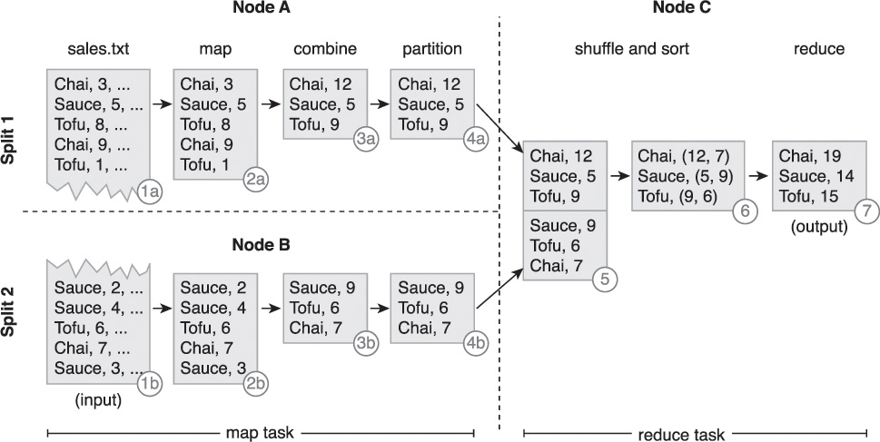
The following steps are shown in Figure 6.18:
1. The input (sales.txt) is divided into two splits.
2. Two map tasks running on two different nodes, Node A and Node B, extract product and quantity from the respective split’s records in parallel. The output from each map function is a key-value pair where product is the key while quantity is the value.
3. The combiner then performs local summation of product quantities.
4. As there is only one reduce task, no partitioning is performed.
5. The output from the two map tasks is then copied to a third node, Node C, that runs the shuffle stage as part of the reduce task.
6. The sort stage then groups all quantities of the same product together as a list.
7. Like the combiner, the reduce function then sums up the quantities of each unique product in order to create the output.
Understanding MapReduce Algorithms
Unlike traditional programming models, MapReduce follows a distinct programming model. In order to understand how algorithms can be designed or adapted to this programming model, its design principle first needs to be explored.
As described earlier, MapReduce works on the principle of divide-and-conquer. However, it is important to understand the semantics of this principle in the context of MapReduce. The divide-and-conquer principle is generally achieved using one of the following approaches:
• Task Parallelism – Task parallelism refers to the parallelization of data processing by dividing a task into sub-tasks and running each sub-task on a separate processor, generally on a separate node in a cluster (Figure 6.19). Each sub-task generally executes a different algorithm, with its own copy of the same data or different data as its input, in parallel. Generally, the output from multiple sub-tasks is joined together to obtain the final set of results.

Figure 6.19 A task is split into two sub-tasks, Sub-task A and Sub-task B, which are then run on two different nodes on the same dataset.
• Data Parallelism – Data parallelism refers to the parallelization of data processing by dividing a dataset into multiple datasets and processing each sub-dataset in parallel (Figure 6.20). The sub-datasets are spread across multiple nodes and are all processed using the same algorithm. Generally, the output from each processed sub-dataset is joined together to obtain the final set of results.
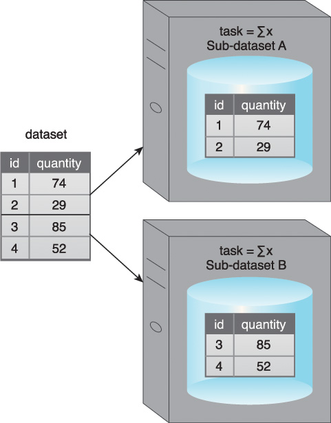
Figure 6.20 A dataset is divided into two sub-datasets, Sub-dataset A and Sub-dataset B, which are then processed on two different nodes using the same function.
Within Big Data environments, the same task generally needs to be performed repeatedly on a data unit, such as a record, where the complete dataset is distributed across multiple locations due to its large size. MapReduce addresses this requirement by employing the data parallelism approach, where the data is divided into splits. Each split is then processed by its own instance of the map function, which contains the same processing logic as the other map functions.
The majority of traditional algorithmic development follows a sequential approach where operations on data are performed one after the other in such a way that subsequent operation is dependent on its preceding operation.
In MapReduce, operations are divided among the map and reduce functions. Map and reduce tasks are independent and in turn run isolated from one another. Furthermore, each instance of a map or reduce function runs independently of other instances.
Function signatures in traditional algorithmic development are generally not constrained. In MapReduce, the map and reduce function signatures are constrained to a set of key-value pairs. This is the only way that a map function can communicate with a reduce function. Apart from this, the logic in the map function is dependent on how records are parsed, which further depends on what constitutes a logical data unit within the dataset.
For example, each line in a text file generally represents a single record. However, it may be that a set of two or more lines actually constitute a single record (Figure 6.21). Furthermore, the logic within the reduce function is dependent on the output of the map function, particularly which keys were emitted from the map function as the reduce function receives a unique key with a consolidated list of all of its values. It should be noted that in some scenarios, such as with text extraction, a reduce function may not be required.

The key considerations when developing a MapReduce algorithm can be summarized as follows:
• Use of relatively simplistic algorithmic logic, such that the required result can be obtained by applying the same logic to different portions of a dataset in parallel and then aggregating the results in some manner.
• Availability of the dataset in a distributed manner partitioned across a cluster so that multiple map functions can process different subsets of a dataset in parallel.
• Understanding of the data structure within the dataset so that a meaningful data unit (a single record) can be chosen.
• Dividing algorithmic logic into map and reduce functions so that the logic in the map function is not dependent on the complete dataset, since only data within a single split is available.
• Emitting the correct key from the map function along with all the required data as value because the reduce function’s logic can only process those values that were emitted as part of the key-value pairs from the map function.
• Emitting the correct key from the reduce function along with the required data as value because the output from each reduce function becomes the final output of the MapReduce algorithm.
Processing in Realtime Mode
In realtime mode, data is processed in-memory as it is captured before being persisted to the disk. Response time generally ranges from a sub-second to under a minute. Realtime mode addresses the velocity characteristic of Big Data datasets.
Within Big Data processing, realtime processing is also called event or stream processing as the data either arrives continuously (stream) or at intervals (event). The individual event/stream datum is generally small in size, but its continuous nature results in very large datasets.
Another related term, interactive mode, falls within the category of realtime. Interactive mode generally refers to query processing in realtime. Operational BI/analytics are generally conducted in realtime mode.
A fundamental principle related to Big Data processing is called the Speed, Consistency and Volume (SCV) principle. It is covered first as it establishes some basic constraints on processing that mainly impact realtime processing mode.
Speed Consistency Volume (SCV)
Whereas the CAP theorem is primarily related to distributed data storage, the SCV (Figure 6.22) principle is related to distributed data processing. It states that a distributed data processing system can be designed to support only two of the following three requirements:
• Speed – Speed refers to how quickly the data can be processed once it is generated. In the case of realtime analytics, data is processed comparatively faster than batch analytics. This generally excludes the time taken to capture data and focuses only on the actual data processing, such as generating statistics or executing an algorithm.
• Consistency – Consistency refers to the accuracy and the precision of the results. Results are deemed accurate if they are close to the correct value and precise if close to each other. A more consistent system will make use of all available data, resulting in high accuracy and precision as compared to a less consistent system that makes use of sampling techniques, which can result in lower accuracy with an acceptable level of precision.
• Volume – Volume refers to the amount of data that can be processed. Big Data’s velocity characteristic results in fast growing datasets leading to huge volumes of data that need to be processed in a distributed manner. Processing such voluminous data in its entirety while ensuring speed and consistency is not possible.

If speed (S) and consistency (C) are required, it is not possible to process high volumes of data (V) because large amounts of data slow down data processing.
If consistency (C) and processing of high volumes of data (V) are required, it is not possible to process the data at high speed (S) as achieving high speed data processing requires smaller data volumes.
If high volume (V) data processing coupled with high speed (S) data processing is required, the processed results will not be consistent (C) since high-speed processing of large amounts of data involves sampling the data, which may reduce consistency.
It should be noted that the choice of which two of the three dimensions to support is fully dependent upon the system requirements of the analysis environment.
In Big Data environments, making the maximum amount of data available is mandatory for performing in-depth analysis, such as pattern identification. Hence, forgoing volume (V) over speed (S) and consistency (C) needs to be considered carefully as data may still be required for batch processing in order to glean further insights.
In the case of Big Data processing, assuming that data (V) loss is unacceptable, generally a realtime data analysis system will either be S+V or C+V, depending upon whether speed (S) or consistent results (C) is favored.
Processing Big Data in realtime generally refers to realtime or near-realtime analytics. Data is processed as it arrives at the enterprise boundary without an unreasonable delay. Instead of initially persisting the data to the disk, for example to a database, the data is first processed in memory and then persisted to the disk for future use or archival purposes. This is opposite of batch processing mode, where data is persisted to the disk first and then subsequently processed, which can create significant delays.
Analyzing Big Data in realtime requires the use of in-memory storage devices (IMDGs or IMDBs). Once in memory, the data can then be processed in realtime without incurring any hard-disk I/O latency. The realtime processing may involve calculating simple statistics, executing complex algorithms or updating the state of the in-memory data as a result of a change detected in some metric.
For enhanced data analysis, in-memory data can be combined with previously batch-processed data or denormalized data loaded from on-disk storage devices. This helps to achieve realtime data processing as datasets can be joined in memory.
Although realtime Big Data processing generally refers to incoming new data, it can also include performing queries on previously persisted data that requires interactive response. Once the data has been processed, the processing results can then be published for interested consumers. This may occur via a realtime dashboard application or a Web application that delivers realtime updates to the user.
Depending on system requirements, the processed data along with the raw input data can be offloaded to on-disk storage for subsequent complex, batch data analyses.
The following steps are shown in Figure 6.23:
1. Streaming data is captured via a data transfer engine.
2. It is then simultaneously saved to an in-memory storage device (a) and an on-disk storage device (b).
3. A processing engine is then used to process data in realtime.
4. Finally, the results are fed to a dashboard for operational analysis.

Two important concepts related to realtime Big Data processing are:
• Event Stream Processing (ESP)
• Complex Event Processing (CEP)
Event Stream Processing
During ESP, an incoming stream of events, generally from a single source and ordered by time, is continuously analyzed. The analysis can occur via simple queries or the application of algorithms that are mostly formula-based. The analysis takes place in-memory before storing the events to an on-disk storage device.
Other (memory resident) data sources can also be incorporated into the analysis for performing richer analytics. The processing results can be fed to a dashboard or can act as a trigger for another application to perform a preconfigured action or further analysis. ESP focuses more on speed than complexity; the operation to be executed is comparatively simple to aid faster execution.
Complex Event Processing
During CEP, a number of realtime events often coming from disparate sources and arriving at different time intervals are analyzed simultaneously for the detection of patterns and initiation of action. Rule-based algorithms and statistical techniques are applied, taking into account business logic and process context to discover cross-cutting complex event patterns.
CEP focuses more on complexity, providing rich analytics. However, as a result, speed of execution may be adversely affected. In general, CEP is considered to be a superset of ESP and often the output of ESP results in the generation of synthetic events that can be fed into CEP.
Realtime Big Data Processing and SCV
While designing a realtime Big Data processing system, the SCV principle needs to be kept in mind. In light of this principle, consider a hard-realtime and a near-realtime Big Data processing system. For both hard-realtime and near-realtime scenarios, we assume that data loss is unacceptable; in other words, high data volume (V) processing is required for both the systems.
Note that the requirement that the data loss should not occur does not mean that all data will actually be processed in realtime. Rather, it means that the system captures all input data and that the data is always persisted to disk either directly by writing it to on-disk storage or indirectly to a disk serving as a persistence layer for in-memory storage.
In the case of a hard-realtime system, a fast response (S) is required, hence consistency (C) will be compromised if high volume data (V) needs to be processed in memory. This scenario will require the use of sampling or approximation techniques, which will in turn generate less accurate results but with tolerable precision in a timely manner.
In the case of a near-realtime system, a reasonably fast response (S) is required, hence consistency (C) can be guaranteed if high volume data (V) needs to be processed in memory. Results will be more accurate when compared to a hard-realtime system since the complete dataset can be used instead of taking samples or employing approximation techniques.
Thus, in the context of Big Data processing, a hard-realtime system requires a compromise on consistency (C) to guarantee a fast response (S) while a near-realtime system can compromise speed (S) to guarantee consistent results (C).
Realtime Big Data Processing and MapReduce
MapReduce is generally unsuitable for realtime Big Data processing. There are several reasons for this, not the least of which is the amount of overhead associated with MapReduce job creation and coordination. MapReduce is intended for the batch-oriented processing of large amounts of data that has been stored to disk. MapReduce cannot process data incrementally and can only process complete datasets. It therefore requires all input data to be available in its entirety before the execution of the data processing job. This is at odds with the requirements for realtime data processing as realtime processing involves data that is often incomplete and continuously arriving via a stream.
Additionally, with MapReduce a reduce task cannot generally start before the completion of all map tasks. First, the map output is persisted locally on each node that runs the map function. Next, the map output is copied over the network to the nodes that run the reduce function, introducing processing latency. Similarly, the results of one reducer cannot be directly fed into another reducer, rather the results would have to be passed to a mapper first in a subsequent MapReduce job.
As demonstrated, MapReduce is generally not useful for realtime processing, especially when hard-realtime constraints are present. There are however some strategies that can enable the use of MapReduce in near-realtime Big Data processing scenarios.
One strategy is to use in-memory storage to store data that serves as input to interactive queries that consist of MapReduce jobs. Alternatively, micro-batch MapReduce jobs can be deployed that are configured to run on comparatively smaller datasets at frequent intervals, such as every fifteen minutes. Another approach is to continuously run MapReduce jobs against on-disk datasets to create materialized views that can then be combined with small volume analysis results, obtained from newly arriving in-memory streaming data, for interactive query processing.
Given the predominance of smart devices and corporate desires to engage customers more proactively, advancements in realtime Big Data processing capabilities are occurring very quickly. Several open source Apache projects, specifically Spark, Storm and Tez, provide true realtime Big Data processing capabilities and are the foundation of a new generation of realtime processing solutions.