IN THIS CHAPTER
Average Cost
COGS and Gross Margin
If your company is a consultancy, or if you provide professional services, or if your use of tangible materials in the production of a product can be sensibly viewed as an expense, then you probably have little use for inventory analysis.
But if you're a retailer, wholesaler, or other type of merchandiser, or if you manufacture products, it's likely that most of your operating profit comes from selling goods for more than your acquisition costs. And in that case, the management and valuation of inventory is critically important to the health of your business.
On the balance sheet, it's likely that inventory represents the majority of a merchandiser's current assets. It can be tricky to weigh the need for inventory availability against the costs of acquiring and keeping it in stock.
On the income statement, the gross profit that a merchandising firm realizes during an accounting period is directly attributable to the difference between sales price and the cost of the goods sold (COGS). If you have a mistaken idea of how much the wireless printer you just sold cost you, you also have a mistaken idea of how much money the sale made you.
QuickBooks has tools that help you keep track of how much money you have invested in inventory, how many units you own, and how fast you turn them over. The tools that help you find out how profitable your company is, in conducting its merchandising or manufacturing business, are also available — they just take a little study to find out how they can inform or mislead you.
The key, in QuickBooks anyway, is the idea that every item in your inventory has an average cost.
The fundamental aspect about the value of your company's inventory assets is that you value a unit according to what you paid for it. There are additional considerations that sometimes apply, such as revaluing your inventory according to lower of cost or market rules, or inventory profits, but even these use your cost of acquisition as a basis.
Note
The lower of cost or market principle is a conservative approach to valuation that states that inventory (or other investments, for that matter) should appear on the balance sheet as worth either the lower of what the company paid for them, or their current replacement cost. Inventory profits come about when inventory is held in stock for a period of time during which the replacement cost rises, and the inventory assets are more valuable than they were when acquired. Inventory profits present accountants with headaches.
Taking acquisition cost as the building block of an inventory analysis, the next issue that arises is the assignment of unit costs. Suppose that you purchased 100 widgets in June for $5 each. You sell one today for $7. Your revenue on that sale is $7, your COGS is $5, and your gross profit is therefore $2. You still have 99 widgets in stock that you paid $5 apiece for, so your total widget asset is worth $495.
Then in July you buy another 100 widgets for $6 each and put them in a store bin along with the 99 widgets remaining from your original acquisition. That bin now contains $1,095 worth of widgets. A customer grabs one and buys it. You charge him $7, as before, but what is your COGS? Your gross profit? And what are your widgets worth now?
If the customer bought a widget that cost you $5, your COGS was $5 and your gross profit was $2. You have $1,090 worth of widgets.
If he bought a widget that cost you $6, your COGS was $6 and your gross profit was $1. Your widgets are worth $1,089.
Obviously this isn't a tenable situation, and the reason is that you have so many widgets in stock, and that they are relatively inexpensive. It's just not worth your while to keep track of the actual acquisition cost of every single unit that you sell, not when the gross profit is in the one- to two-dollar range.
If you sold custom made surfboards instead of widgets, if you had twenty in stock at any given time and they cost anywhere from $500 to $600 to build, then it might make sense to keep track of the cost of acquiring each one. And this inventory valuation method is used by merchandisers such as jewelers, fine art studios, and classic car dealers — virtually any merchandiser who deals in relatively small numbers of relatively expensive goods. It even has a name: specific identification. QuickBooks does not do a good job of supporting the specific identification method of valuing inventory. It can be done, but you have to jump through hoops.
Note
Specific identification in large-volume, low-cost situations has become more feasible as point-of-sale scanners that can identify unique units have become more common. But that doesn't help in situations where you cannot point to a unique unit with a unique acquisition cost. A gallon of gasoline, for example.
Another approach that many companies use is FIFO, which stands for first in, first out. (There is also the reverse approach, LIFO, or last in, first out, that is much more controversial than FIFO.) Under FIFO, you assume that, in the prior example, your customer bought a widget that cost you $5, even though the bin is stocked with both $5 and $6 widgets.
You will continue to assume that your customers are buying $5 widgets until you have sold 100 widgets, the size of your initial buy. At that point you will assume that the next widget sold cost you $6. First in, first out: You assume that you sell nothing but the first batch until you have sold all of them. Only then does the opposite side of the assumption kick in: Until you sell as many units as were in the second batch, that's all you're selling. Under FIFO, you act as though your customers have entered into an agreement with you to pull the oldest widgets out of the bin first.
Even jumping through hoops won't help you here: QuickBooks has no feasible way to track inventory value using FIFO. What about a custom field? At the time of this writing, custom fields in QuickBooks are text-only and will do you no good in tracking inventory with FIFO methods.
The third broadly defined approach to inventory valuation is average cost. You bought 100 widgets for $5 and 100 for $6. Setting aside for a moment the issue of how many you have sold, one way of looking at it is that you bought 200 widgets for a total of $1,100, so the unit cost of any one of those widgets is the average cost, $1,100 ÷ 200, or $5.50.
That average cost is used as the basis for the COGS. If you sell one widget for $7, your COGS is $5.50 and your gross profit is $1.50. Those figures hold true until you buy more widgets at a cost that's something more or less than $5.50 each, whether or not you have run out of widgets.
It's at this point that the basic concept of average cost becomes more complicated. There are two schools of thought about whether or not sales should influence average cost, and each is associated with a different calculation method. Both pass muster with GAAP (Generally Accepted Accounting Practices) but they can yield very different results. I describe them both, starting with the method that QuickBooks does not use, but that I'll refer to as the "mainstream" approach to average costing.
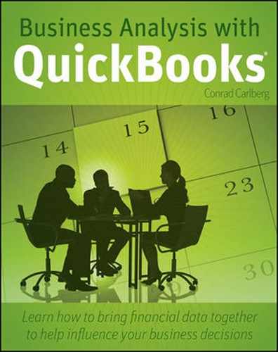
Using the mainstream approach to average costing, all you do is add up the cost of the units of a given product you have purchased to inventory. Then you count the number of units you bought. You divide the first number by the second, and that's your average cost. Figure 7.1 shows how this approach would calculate the average cost of your widgets.
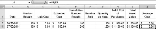
Figure 7.1. Excel's formula box shows the formula in the active cell. It divides total purchases by units purchased.
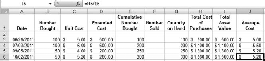
Figure 7.1 shows a situation that's about as simple as it gets. On any given date, you add up the dollars you spent and divide by the number you bought.
At any rate, that's the theory. It does get a little more complicated in practice, but only a little. Figure 7.2 complicates matters by adding more purchases at different unit costs.
In Figure 7.2, you see average cost change each time another purchase is made at a cost per unit that differs from the current average cost. It doesn't matter how many units are purchased. It doesn't matter whether any units have been sold. Under this approach, if you buy more stock at a unit cost that's different from the current average cost, the average cost changes, and not otherwise.
Figure 7.2 shows the average cost changing in response to the purchase in July and the purchase in September, each of which is made at a unit cost that differs from the average cost immediately prior to the date of the purchase. The fourth purchase is made at a unit cost of $5.20, that equals the average cost immediately prior to the purchase — and therefore the average cost does not change.
Figure 7.3 shows what happens — or, rather, what doesn't happen — when you sell some units.
You see in Figure 7.3 that 100 widgets have been sold in August. That sale has no effect on the average cost — notice that the average cost on the date of the sale is unchanged, and that the average costs following the sale are the same as they would be had the sale not occurred — compare to the average cost figures in Figure 7.2.
Notice, by the way, the COGS associated with the sale made in August shown in Figure 7.3. You can get COGS quickly by comparing the Total Asset Value prior to the sale, in cell I4, with the Total Asset Value as of the sale, in cell I5. The difference is $1,100 – $550, or $550. The COGS for the sale is $550. It is also the result of multiplying the number of units sold, 100, by the average cost just prior to the sale, $5.50.
And that is how QuickBooks arrives at a COGS figure (even though it uses a different method of calculating average cost). QuickBooks multiplies the number of units sold by their average cost to get the COGS. That value is subtracted from the prior Total Asset Value to get a new Total Asset Value. The COGS is also subtracted from the sales price to arrive at a gross profit for the sale.
The average cost formula explained in this section is acceptable under GAAP as a measure of average cost. There are several reasons that many users find it preferable to the approach that QuickBooks uses. Here are three:
It is the true average cost of all the items you brought into inventory, not just the items you currently have in stock.
It is easier to verify because it is not affected by sales of the item.
It is not subject to fluctuations that are as extreme as can occur using the QuickBooks formula, because it uses information about all the purchases of the item that you have made.
QuickBooks adopts a different approach to calculating the average cost of an item. It too is approved by GAAP, but it would be more accurate to call it " average cost of items on hand." The difference between the QuickBooks method and the mainstream method is that QuickBooks adjusts the number purchased and the total acquisition cost according to any sales that have taken place. Figure 7.4 shows how the QuickBooks approach to average cost changes the outcomes of the transactions shown in Figure 7.3.

Figure 7.4. Compare with Figure 7.3. The difference so far is only in average cost after the first sale, in August.
The calculation of average cost by the mainstream approach uses the formula:
Average Cost = (Total Purchase Cost) / (Total Quantity Purchased)
In contrast, QuickBooks calculates the current average cost of an inventory item as:
Average Cost = (Total Asset Value) / (Quantity on Hand)
An item's asset value is the total acquisition cost of that item less the total COGS, taking into account such transactions as Inventory Adjustments that can change the dollar value of an item's stock. The item's quantity on hand works the same way, but it is a count of the number of units rather than a total of the dollars currently invested in the units.
One consequence of using this formula is that it makes average cost sensitive to the sales of an item — the formula uses on-hand values, which are the result of combining purchases with sales. This fact is often hidden in the numbers, because you don't usually see a change in an item's average cost until you buy more of it at a different unit cost. A sale affects both the quantity on hand and the total asset value, and therefore it will eventually have an effect on average cost, but not before another purchase is made at a unit cost that differs from the current average cost.
When you sell an item, both its asset value and the quantity on hand change — but its average cost doesn't, because the ratio of value to quantity remains the same. If you start with 100 units at $5 each, and sell 90, the average cost remains unchanged: ($500 ÷ 100 units) gives the same average cost as does the ratio of the resulting total asset value and quantity on hand ($50 ÷ 10 units). Even though there's no apparent change at this point, the sale has an effect on the average cost later on, when you buy more units at a different price.

In Figure 7.4, the sale of 100 units in August had no immediate effect on the average cost of $5.50, because it did not change the ratio of asset value to quantity on hand. But when the next purchase was made in September, the average cost changed to $5.00 (because September's unit cost of $4.00 is lower than the existing average cost of $5.50) and it is different from the average cost of $5.20 shown in Figure 7.3 because of the differences in the formulas used.
Figure 7.5 returns to the mainstream approach to average costing. Notice that 100 widgets were sold in November. The average cost did not change, because under the mainstream approach sales have no effect on average cost. The asset value changes though, from $1,040 to $520, a drop of $520. That $520 is the COGS for the sale. QuickBooks arrives at the COGS by multiplying the units sold, 100, by the current average cost, $5.20.
Now compare Figure 7.5 with Figure 7.6, which shows how QuickBooks handles the November sale of 100 widgets.
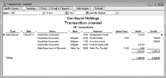
In Figure 7.6, the COGS for the November sale is ($1,010 – $505), or $505. In Figure 7.5, that sale's COGS is $520. The method of calculating COGS, and for calculating gross profit, is the same regardless of which method you use to calculate average cost. But because the two methods calculate average cost differently, the results of the COGS and gross profit calculations differ. Figure 7.7 shows the journal entry for the sale, including QuickBooks' calculation of the COGS.
Using the QuickBooks approach, it's not always easy to figure out why a current average cost has the value it does. You have to track all the increases and the decreases to your holding in a given item — all the purchases, sales, adjustments to quantity, adjustments to valuation, and so on — or you won't arrive at the same figure as QuickBooks.
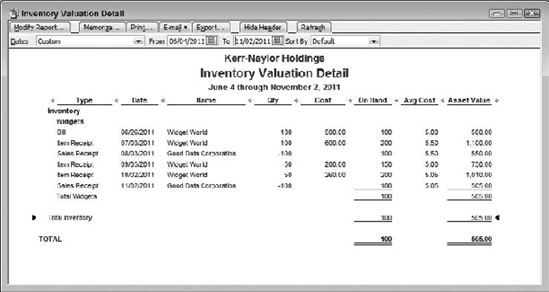
Figure 7.6. The average cost calculated by QuickBooks differs from the calculation shown in Figure 7.5, and therefore the COGS and gross profit are different.
There is no danger posed to your company's bottom line by the choice of method to calculate average cost. The method employed by QuickBooks tends to result in a more volatile measure of average cost, and people who have not encountered the QuickBooks method before sometimes have difficulty determining what's going on with their inventory valuation.
But in the long run, neither method is superior to the other as a means of determining COGS for the income statement or the asset value for the balance sheet. Particularly from the standpoint of the taxing authorities, what really matters is to be consistent across product lines and over time.
With all that said, QuickBooks introduces a problem that, if you don't understand its consequences, can immediately create huge headaches for you. Those headaches do nothing but get worse if you don't fix the problem right away. The problem concerns selling more of an item than QuickBooks thinks you have in stock: that is, selling negative. If you sell more of an item than is currently available, that error interacts with the method of calculating average cost. It does so in a way that makes it impossible for you to trust any financial results for that item that come about following the date of the error.
Merely selling out of an item is hardly a catastrophe — not, at least, to your financial statements. It can make you scratch your head when you look at an item's average cost, but if you acquire more of the item, or deactivate or otherwise discontinue it, no harm is done. Still, it will help to understand what's going on with the relatively benign act of selling to exactly zero units on hand.
When you sell an item down to a zero quantity and then replenish your supply at a different cost, the inventory valuation can appear to be out of whack. If you look again at the formula that QuickBooks uses:
Average Cost = (Total Asset Value) / (Quantity on Hand)
You see that when an item goes to zero units on hand its average cost is undefined — because you'd be dividing by zero — and that's why QuickBooks temporarily uses the existing average cost. See Figure 7.8 where a sale made in December takes the company's quantity on hand to zero.
Then, when you replenish your supply, the new average cost is based entirely on the cost of that new purchase. The history of prior purchases disappears from the average cost estimate, which is based solely on the units you currently own. Figure 7.9 shows what happens to the average cost when, in January, the company buys 100 widgets at $3 each.

Figure 7.8. You may wonder how an item can have any average cost at all when the average's numerator and denominator are both zero.
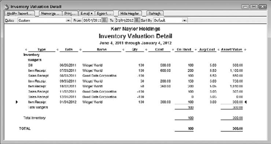
Figure 7.9. The new average cost, after an item has been taken to zero and then replenished, is that purchase's unit cost.

Figure 7.10. The new average cost retains the effect of the purchases made before taking the item to a zero quantity.
The current average cost of $3.00, as shown in Figure 7.9, no longer comprises any of the item's prior history. You may or may not regard that effect as desirable. Many users and accountants do not, primarily because this version of average cost is much more volatile when your suppliers are changing the prices they charge you. (GAAP takes no position on the issue of which version is preferable.)
Figure 7.10 is provided so that you can contrast the effects of the two formulas.
So far, what you've seen concerning inventory valuation is entirely due to the two different methods of calculating the average cost of an inventory item:
(Total Purchase Cost) / (Total Units Purchased)
and
(Total Asset Value) / (Quantity on Hand)
The differences in asset valuation are entirely due to different concepts of what should constitute the average cost of an item (the method used by QuickBooks actually has a lot of FIFO in it). But QuickBooks has a quirk that magnifies the effect of the differences you've seen so far. That quirk is the fact that QuickBooks allows the user to sell negative, by selling more of an item than is on hand — and this is nowhere near as benign as just depleting your stock.
Suppose you have 10 widgets on hand and a customer wants to buy 20. Maybe the customer doesn't need them all right away, or maybe you can borrow ten more from another order that isn't scheduled to ship for a couple of days, or maybe you've just completed a physical inventory and you know that QuickBooks has a short count. Whatever your rationale, you use QuickBooks to establish a sales receipt or invoice transaction that calls for the sale of 10 more widgets than QuickBooks shows you presently have on hand.

Figure 7.11. The negative quantity on hand in February will freeze the average cost, but not the asset value.
If you've done that before, whether deliberately or by accident, you know that QuickBooks Pro displays the message "You don't have sufficient quantity available to sell 20 of the item: Widgets," where the quantity and the name of the item depends on how much you tried to sell of which item. (The message may be different if you're using QuickBooks Premier, but its substance is the same.) There's an OK button, and after you click it you're back at the Sales Receipt window. Click the Save and Close button and you have succeeded in selling more widgets than QuickBooks thinks you have in stock. QuickBooks now declines, and continues to decline, to recalculate the current average cost for widgets until the quantity on hand turns positive again. Figure 7.11 shows your current inventory situation, with a negative quantity on hand.
Now, suppose you buy five more widgets, at a cost that's different from the current average cost. According to the QuickBooks formula for average cost, this should result in a change in the average cost. Figure 7.12 shows that it actually doesn't.
You've bought five units at $100 each — roughly 20 times what you had been paying. But the average cost doesn't budge. Remember: Average cost won't change until the quantity on hand is once again greater than zero. One consequence of the unchanging average cost appears in the total asset value. You spent $500, but the asset value has increased by only $15.00. That increase of $15.00 occurs because QuickBooks uses the old average cost of $3.00 to calculate the effect of your $500 purchase on the asset value: the acquisition of five units at an out-of-date average cost of $3.00 results in an increase in asset value of $15.00, rather than the actual increase of $500 due to purchasing five units for $100 each.

The effect is not limited to asset valuation, but, as you might expect, there's a consequence for COGS and gross profit as well. Figures 7.13 and 7.14 show that when you make another sale and the current quantity on hand is already below zero, the COGS can be based on an erroneous average cost. Figure 7.13 shows the inventory report, and Figure 7.14 shows the journal entry associated with the sale.
Here's what happened. First, using the QuickBooks version of average cost:
Starting in November 2011, the first two sales transactions are entirely normal: You sell 100 units, dropping the quantity on hand to 100, and then sell another 100, completely selling out of the item. As explained earlier, the result of selling to exactly zero is to set the average cost to the same value it had prior to that transaction. In this case, that's $5.05. The purchase of another 10 widgets on 1/3/2012 takes you back into positive territory and resets the average cost based exclusively on that purchase, that is $3.00.
But then, on 2/1/2012, you sell another 20 units. That's 10 more than you had on hand, and you are now in negative territory. Notice that the Total Asset Value is correct. (But that's an accident: Even a broken clock is right twice a day.) You have −10 units, and at an Average Cost of $3, the Asset Value is –$30.00. Nothing has happened so far to change the Average Cost. Remember, sales have no immediate effect on Average Cost.
Now, on 3/1/2012, you buy five units for $500.00. That's $100 apiece, and two errors jump out at you:
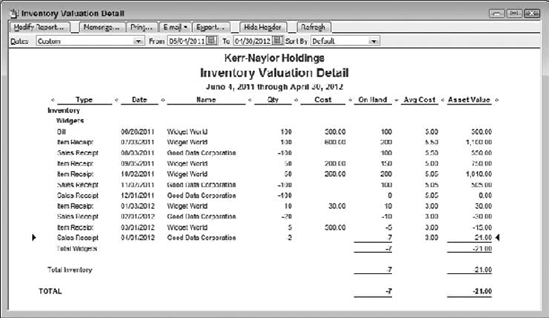


Figure 7.15. The misstatement of COGS is the kind of damage that can be caused by selling into a negative quantity on hand.
The Average Value should change from $3, but it does not: You still see an Average Value of $3 as of the purchase.
The Total Asset Value is now also wrong: The numeric accident that caused an erroneous calculation to return a correct result can't recur when the true average cost has changed.
The quantity on hand is correct, but both the Average Cost and the Total Asset Value are wrong. Again: QuickBooks does not recalculate Average Cost when the quantity on hand is zero or below.
You haven't suffered financial damage yet, but you're about to. On 4/1/2012, you sell two units, taking you from −5 on hand to −7 on hand. Because you still have a negative quantity on hand, QuickBooks doesn't yet recalculate the Average Cost. And because you sold two units on 4/1/2012, QuickBooks assigns a COGS of $6 to that sale. Figure 7.15 shows the relevant journal entry.
The journal's COGS entry says that you sold, for $240, inventory items that cost you $6 to acquire. But which physical units did you sell? You had −10 units on 2/1/2012, and although you can sell imaginary units, you can't sell physical units you don't have, so the sale can't have been from the −10 units. So, on 4/1/2012 you must have sold two of the five units you bought on 3/1/2012. You bought them for $100 apiece — but QuickBooks thinks the sale's COGS was $6.
Your apparent gross margin on that sale was therefore $240 revenue less $6 COGS, or $234. You'll be obligated to pay corporate income tax on that profit, after it has been reduced to taxable income by legitimate deductions. But those two widgets actually cost you $200, so in fact your gross margin was $40. From just about every standpoint that you can name — taxes, cash flow, product line analysis — you have problems that are directly traceable to the combination of QuickBooks' method of average costing combined with its feckless response to the act of selling more than you appear to have.

Figure 7.16. You wouldn't know until your accountant told you that something was wrong, unless you make a habit of looking at more than just the current month.
Finally, on 5/1/2012, your quantity on hand turns positive again as you buy 10 more units. And QuickBooks responds by recalculating the Average Cost, although you can't tell that it did, because that purchase is for $3 per unit — the same as the Average Cost that was current before all the quantity on hand went negative and you transacted business with some very different cost structures (see Figure 7.16).
Note
I could have demonstrated that the Average Cost calculation kicks back in on 5/1/2012 by arranging a purchase at a different unit cost, such as $9, instead of $3. I did it this way to demonstrate how what's really happening with QuickBooks' Average Costs can be masked by the numbers.
The best way to avoid these problems is to avoid letting an inventory item go negative at all. There are two general ways to do that: before and after. If you can arrange things so that your apparent quantity on hand doesn't dip below zero, you're managing your inventory before anything bad happens. If for some reason you can't avoid a negative quantity on hand, you can still recover after the fact, but it may take some extra work.
One of the differences between the QuickBooks Pro and Premier editions is support for sales orders — which can be much like backorders, if you're more comfortable with that term. Using QuickBooks Pro, you can emulate Sales Orders as they're handled in a QuickBooks Premier edition — it's just not quite as convenient and you can't duplicate all the functionality.
There are several steps you can take, including establishing a custom field, that make it easier to work with backorders in QuickBooks Pro. Because this book is not intended as a users' guide, I'll skip the details, and just mention the irreducible minimums for dealing with insufficient inventory in Pro and Premier.
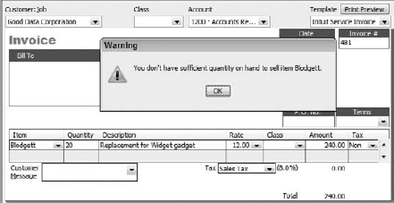
When you create a Sales Receipt or an Invoice in QuickBooks Pro that involves the sale of inventory items, you must enter the number of units of each item you're selling. If you try to sell more units than you have recorded in QuickBooks as on hand, you see the message shown in Figure 7.17.
When you click OK, the warning disappears and you can continue editing the transaction. Before you save it, though, you should right-click the form's header or footer, or click the Edit menu, and select Mark Invoice as Pending. (If you're creating a Sales Receipt, the menu item is Mark Sales Receipt as Pending.)
When you do so, a Pending stamp appears on the form (see Figure 7.18). A pending invoice or sales receipt is known as a " nonposting" transaction. No journal entries occur when you establish a nonposting transaction, and the inventory unit counts are unaffected. This means that you do not create a negative quantity on hand situation, and all the troubles explained earlier in this chapter are prevented, at least for that transaction.
When you know you once again have sufficient inventory, open the order, right-click the header or footer (or use the Edit menu) and choose Mark Order as Final. Now, when you close the order, the numbers post to the proper accounts, and the COGS and average costs will reflect the reality of your inventory status.
Tip
A quick way to access pending sales is to choose Reports
QuickBooks Premier Edition includes a nonposting transaction called a Sales Order. You can think of a sales order as a way to collect information about a sale without actually committing it to your company's financial records. Only when the sales order is finalized by turning it into an invoice is the revenue recognized and the posting to various accounts performed.

There are various reasons that a company might want to delay recognizing revenue temporarily. The customer might have a large balance due, or a sales manager might want to watch a new sales rep more closely than usual. Or, insufficient inventory might come into play.
If a possible shortage of inventory is the reason for creating a sales order instead of a sales receipt or an invoice, there are additional benefits to Premier's sales orders that are not available in Pro. For example, you can arrange to distinguish between quantity available and quantity on hand. Quantity on hand, in this context, is the number of units on the shelf, ready to ship. Quantity available, by contrast, is the number of units ready to ship that have not already been spoken for by other sales, sales orders, or assembly builds.
In any case, if you enter into a sales order more units of an inventory item than can be shipped, you'll be warned as you are using QuickBooks Pro. It's necessary to have enabled the warning (choose Edit
As with Sales Receipts and Invoices in QuickBooks Pro, you can put a Pending stamp on a sales order from a contextual menu by right-clicking the order's header or footer. In the case of sales orders, though, it's less critical because a sales order is by definition a nonposting transaction.
The main point to keep in mind is that QuickBooks offers you tools that help you record information about a sale without actually committing you to fulfilling it. At the very least, a pending sale or a sales order is an important buffer that can prevent the inventory count on an item from going negative.
A customer has called to tell you he wants to buy all your remaining stock of Princess phones. QuickBooks has warned you that you don't have a sufficient quantity to sell even one, but you know perfectly well that you have had 10 of them gathering dust in dead storage since Ford pardoned Nixon. You'd love to unload them (the phones) and you do so, ignoring the QuickBooks warning that you don't have enough on hand.
Now comes the hangover. QuickBooks thinks you're even farther into negative territory on that item than you were before. The phones' average cost showed up as $75 — a legitimate figure as of your most recent acquisition but not since. You got rid of the phones for a token $100 but the COGS appear in the Journal as $750. And there's no longer a reference market if you wanted to mark them down via a lower-of-cost-or-market adjustment.
Nevertheless, you should do something about it. There are three approaches that QuickBooks would let you take:
Choose Lists
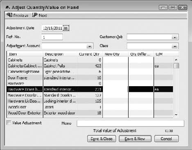
If your quantity adjustment brings the quantity on hand back into positive territory before the date of the sale, the average cost calculation will reflect any subsequent item purchases and the COGS for the sale will be recalculated accordingly. The basic mechanism is the one already mentioned several times: QuickBooks does not recalculate average cost (and therefore does not recalculate COGS) until the quantity on hand is greater than zero.
Using an Inventory Adjustment could be the best approach if the reason that QuickBooks thinks you have fewer than zero units is an erroneous physical inventory.
Another reason you might show a negative quantity on hand is that you bought more units than you told QuickBooks about. There's nothing unusual about a typographical error and if all you did was type 50 instead of 150, there's nothing wrong with correcting it directly in the Item Receipt. You might want to note in the Memo field that it's a corrected record. If this typo caused a negative quantity on hand, it's very likely that correcting it will turn that quantity positive so that QuickBooks can recalculate subsequent average costs and COGS.
It's entirely possible that a prior sales record that took you into negative territory is itself wrong. If it states that you sold 100 blodgetts when in fact you sold 10, it could be that correcting the sales receipt or invoice is all that's needed to correct your quantity on hand to a positive value and cause QuickBooks to recalculate subsequent average costs and COGS figures.