
We can trace the A1 style of referencing back to VisiCalc. Dan Bricklin and Bob Frankston used A1 to refer to the cell in the upper-left corner of the spreadsheet. Mitch Kapor used this same addressing scheme in Lotus 1-2-3. Upstart Multiplan from Microsoft attempted to buck the trend and used something called R1C1-style addressing. In R1C1 addressing, the cell known as A1 is referred to as R1C1 because it is in Row 1, Column 1.
With the dominance of Lotus 1-2-3 in the 1980s and early 1990s, the A1 style became the standard. Microsoft realized it was fighting a losing battle and eventually offered either R1C1-style addressing or A1-style addressing in Excel. When you open Excel today, the A1 style is used by default. Officially, however, Microsoft supports both styles of addressing.
You would think that this chapter would be a nonissue. Anyone who uses the Excel interface would agree that the R1C1 style is dead. However, we have what on the face of it would seem to be an annoying problem: The macro recorder records formulas in the R1C1 style. So, you might be thinking that you just need to learn R1C1 addressing so that you can read the recorded code and switch it back to the familiar A1 style.
I have to give Microsoft credit. After you understand R1C1-style formulas, they are actually more efficient, especially when you are dealing with writing formulas in VBA. Using R1C1-style addressing allows you to write more efficient code. Plus, there are some features, such as setting up array formulas or conditional formatting with the Formula Is option, where you are required to enter the formula in R1C1 style.
I can hear the collective groan from Excel users everywhere. I would be all for skipping 14 pages of this old-fashioned addressing style if it were only an annoyance or an efficiency issue. However, because it is necessary to understand R1C1 addressing to effectively use important features such as array formulas or conditional formatting, we have to dive in and learn this style.
To switch to R1C1-style addressing, select Excel Options from the Office icon menu. In the Formulas category, check the box for R1C1 reference style (see Figure 6.1).

After you switch to R1C1 style, the column letters A, B, C across the top of the worksheet are replaced by numbers 1, 2, 3 (see Figure 6.2).
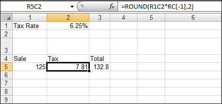
In this format, the cell that you know as B5 is called R5C2 because it is in Row 5, Column 2.
Every couple of weeks, someone manages to accidentally turn this option on, and we get an urgent support request at MrExcel; the style is very foreign to 99 percent of spreadsheet users.
Automatically recalculating thousands of cells is the main benefit of electronic spreadsheets over the green ledger paper used up until 1979. However, I would say a close second prize award would be that you can enter one formula and copy that formula to thousands of cells.
Consider this simple worksheet in Figure 6.3. Enter a simple formula like =C4*B4 in Cell D4, double-click the AutoFill handle, and the formula intelligently changes as at is copied down the range.

The formula in F4 includes both relative and absolute formulas:
=IF(E4,ROUND(D4*$B$1,2),0). Thanks to the dollar signs inserted in B1, you can copy this formula down, and it always multiplies the Total Price in this row by the tax rate in Cell B1.
The numeric results in Figure 6.4 are achieved by the formulas shown in Figure 6.5. (Ctrl+` in Excel switches between Normal view and Formula view.) Considering that I had to enter formulas only in Rows 4 and 10, I think it is amazing that Excel was able to intelligently copy the formulas down the column.
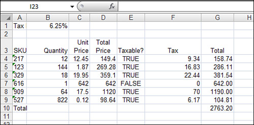

As Excel users, we take this behavior for granted, but people in my beginning Excel class are fairly amazed that the formula =F4+D4 in Cell G4 automatically changed to =F5+D5 when it was copied to Cell G5.
Remember that Excel does everything in R1C1-style formulas. Excel shows addresses and formulas in A1 style merely because it needs to adhere to the standard made popular by VisiCalc and Lotus.
If you switch the worksheet in Figure 6.5 to use R1C1 notation, you will notice that the “different” formulas in D4:D9 are all actually identical formulas in R1C1 notation. The same is true of F4:F9 and G4:G9. Use the Options dialog to change the sample worksheet to R1C1-style addresses. If you examine the formulas in Figure 6.6, you will see that in R1C1 language, every formula in Column D is exactly identical. Given that Excel is storing the formulas in R1C1 style, copying them, and then merely translating to A1 style for us to understand, it is no longer that amazing that Excel can easily manipulate A1-style formulas as it does.

This is one of the reasons that R1C1-style formulas are more efficient in VBA. You can enter the same formula in an entire range of data in a single statement.
An R1C1-style reference includes the letter R to refer to row and the letter C to refer to column. Because the most common reference in a formula is a relative reference, let’s look at relative references in R1C1 style first.
Imagine you are entering a formula in a cell. To point to a cell in a formula, you use the letters R and C. After each letter, enter the number of rows or columns in square brackets.
The following list explains the “rules” for using R1C1 relative references:
For columns, a positive number means to move to the right a certain number of columns, and a negative number means to move to the left a certain number of columns. From cell E5, use
RC[1]to refer to F5 andRC[-1]to refer to D5.For rows, a positive number means to move down the spreadsheet a certain number of rows. A negative number means to move toward the top of the spreadsheet a certain number of rows. From cell E5, use
R[1]Cto refer to E6 and use cellR[-1]Cto refer to E4.If you leave off the square brackets for either the
Ror theC, it means that you are pointing to a cell in the same row or column as the cell with the formula.If you enter
=R[-1]C[-1]in cell E5, you are referring to a cell one row up and one column to the left. This would be cell D4.If you enter
=RC[-1]in cell E5, you are referring to a cell in the same row, but one column to the left. This would be cell D5.If you enter
=RC[1]in cell E5, you are referring to a cell in the same row, but one column to the right. This would be cell F5.If you enter
=RCin cell E5, you are referring to a cell in the same row and column, which is cell E5 itself. You would generally never do this because it would create a circular reference.
Figure 6.7 shows how you would enter a reference in cell E5 to point to various cells around E5.

You can use R1C1 style to refer to a range of cells. If you want to add up the 12 cells to the left of the current cell, the formula is this:
=SUM(RC[-12]:RC[-1])
An absolute reference is one where the row and column remain fixed when the formula is copied to a new location. In A1-style notation, Excel uses a $ before the row number or column letter to keep that row or column absolute as the formula is copied.
To always refer to an absolute row or column number, just leave off the square brackets. This reference refers to cell $B$2 no matter where it is entered:
=R2C2
A mixed reference is one where the row is fixed and the column is allowed to be relative, or where the column is fixed and the row is allowed to be relative. In many situations, this will be useful.
Imagine you’ve written a macro to import Invoice.txt into Excel. Using .End(xlUp), you find where the total row should go. As you are entering totals, you know that you want to sum from the row above the formula up to Row 2. The following code would handle that:
Sub MixedReference()
    TotalRow = Cells(Rows.Count, 1).End(xlUp).Row + 1
    Cells(TotalRow, 1).Value = "Total"
    Cells(TotalRow, 5).Resize(1, 3).FormulaR1C1 = "=SUM(R2C:R[-1]C)"
End Sub
In this code, the reference R2C:R[1]C indicates that the formula should add from Row 2 in the same column to the row just above the formula in the current column. Do you see the advantage to R1C1 formulas in this case? A single R1C1 formula with a mixed reference can be used to easily enter a formula to handle an indeterminate number of rows of data (see Figure 6.8).

You will occasionally write a formula that refers to an entire column. For example, you might want to know the maximum value in Column G. If you don’t know how many rows you will have in G, you can write =MAX($G:$G) in A1 style or =MAX(C7) in R1C1 style. To find the minimum value in Row 1, use =MIN($1:$1) in A1 style or =MIN(R1) in R1C1 style. You can use relative reference for either rows or columns. To find the average of the row above the current cell, use =AVERAGE(R[-1]).
After you get used to R1C1-style formulas, they actually seem a lot more intuitive to build. One classic example to illustrate R1C1-style formulas is building a multiplication table. It is easy to build a multiplication table in Excel using a single mixed-reference formula.
Enter the numbers 1 through 12 going across B1:M1. Copy and transpose these so the same numbers are going down A2:A13. Now the challenge is to build a single formula that works in all cells of B2:M13 and that shows the multiplication of the number in Row 1 times the number in Column 1. Using A1-style formulas, you must press the F4 key five times to get the dollar signs in the proper locations. The following is a far simpler formula in R1C1 style:
Sub MultiplicationTable()
    ' Build a multiplication table using a single formula
    Range("B1:M1").Value = Array(1, 2, 3, 4, 5, 6, 7, 8, 9, 10, 11, 12)
    Range("B1:M1").Font.Bold = True
    Range("B1:M1").Copy
    Range("A2:A13").PasteSpecial Transpose:=True
    Range("B2:M13").FormulaR1C1 = "=RC1*R1C"
    Cells.EntireColumn.AutoFit
End Sub
The R1C1-style reference =RC1*R1C couldn’t be simpler. In English, it is saying, “Take this row’s Column 1 and multiply it by Row 1 of this column.” It works perfectly to build the multiplication table shown in Figure 6.9.

Note
After running the macro and producing the multiplication table in Figure 6.9, note that Excel still has the copied range from line 2 of the macro as the active clipboard item. If the user of this macro would select a cell and press Enter, the contents of those cells would copy to the new location. This is generally not desirable. To get Excel out of Cut/Copy mode, add this line of code before your programs ends:
Application.CutCopyMode = False
Try this experiment. Move the cell pointer to F6. Turn on macro recording using the Record Macro button on the Developer ribbon. Click the Use Relative Reference button on the Developer ribbon. Enter the formula =A1 and press Ctrl+Enter to stay in F6. Click the Stop Recording button on the floating toolbar.
You get this single-line macro, which enters a formula that points to a cell five rows up and five columns to the left:
Sub Macro1()
    ActiveCell.FormulaR1C1 = "=R[-5]C[-5]"
End Sub
Now, move the cell pointer to cell A1 and run the macro that you just recorded. You might think that pointing to a cell five rows above A1 would lead to the ubiquitous Run Time Error 1004. But it doesn’t! When you run the macro, the formula in cell A1 is pointing to =XFA1048572, meaning that R1C1-style formulas actually wrap from the left side of the workbook to the right side. I cannot think of any instance where this would be actually useful, but for those of you who rely on Excel to error out when you ask for something that doesn’t make sense, be aware that your macro will happily provide a result, and probably not the one that you expected!
I like these formulas enough to use them regularly in VBA. I don’t like them enough to change my Excel interface over to R1C1-style numbers. So, I routinely have to know that the cell known as U21 is really R21C21.
Knowing that U is the twenty-first letter of the alphabet is not something that comes naturally. We have 26 letters, so A is 1 and Z is 26. M is the halfway point of the alphabet and is Column 13. The rest of the letters are pretty nonintuitive. I found that by playing this little game for a few minutes each day, I soon had memorized the column numbers:
Sub QuizColumnNumbers()
Do
i = Int(Rnd() * 26) + 1
Ans = InputBox("What column number is the letter " & Chr(64 + i) & "?")
If Ans = "" Then Exit Do
If Not (Ans + 0) = i Then
MsgBox "Letter " & Chr(64 + i) & " is column # " & i
End If
Loop
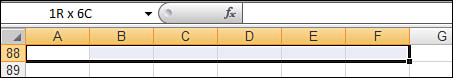
End SubIf you don’t think that memorizing column numbers sounds like fun, or even if you have to figure out the column number of Column DG someday, there is a fairly easy way to do so using the Excel interface. Move the cell pointer to cell A1. Hold down the Shift key and start pressing the right-arrow key. For the first screen of columns, the column number appears in the name box to the left of the formula bar (see Figure 6.10).
As you keep pressing the right-arrow key beyond the first screen, a tool tip box to the right of the current cell tells you how many columns are selected. When you get to Column CS, it informs you that you are at Column 97 (see Figure 6.11).

When you set up conditional formatting, it is important to use R1C1-style formulas. This is not a well-documented statement. The problem is intermittent, but I find that 1 out of every 50 cells set up with conditional formatting will exhibit strange behavior if you use A1-style formulas. When Excel is presented with a conditional formatting rule that looks like it might contain an R1C1 style formula, Excel assumes it is using R1C1 style references. The problem is that some A1 style references, such as R2 to mean a single cell, can be ambiguously interpreted as an R1C1 style reference to all of Row 2.
The Excel user interface emphasizes conditional formatting in which the format of the cell is based on the value in that cell. For most of the conditional formatting options shown in Figure 6.12, Excel simply has to look at the value in the current cell.

In Excel 2007, Microsoft introduced several conditional formatting options in which the format of the cell is based on the comparison between the cell and other cells in the selected range. For example, Duplicate Values or Above Average are new conditional formats in which Excel has to compare each cell to others in a range. All the new visualizations, such as data bars, color scales, and icon sets, compare each cell to the other cells in the range.
However, there is another powerful type of conditional formatting where the format is based on a formula and that formula can point outside of the range. In Excel 97-2003, you would change the first dropdown in the Conditional Format dialog from Cell Value Is to Formula Is. Many people never noticed this dropdown and never found the powerful conditional formatting. In Excel 2007, the option is equally well hidden. You have to select Conditional Formatting, Highlight Cells Rules, More Rules. In the New Formatting Rule dialog, choose the last option in the list, Use a Formula to Determine Which Cells to Format (see Figure 6.13). The formula syntax allows you to build any formula or function that evaluates to True or False. This formula may point to cells other than the current cell, or it may combine multiple conditions with the OR or AND function.

Here is a fairly advanced example. We want to hide any error cells and then color negative numbers in red. The basic idea is to set up a conditional format that checks to see whether the cell contains an error or NA. If either is true, we set the font color up to match the background. This first condition relies on the Formula Is syntax. The second condition is straightforward and relies on the Cell Value Is syntax. Figure 6.14 shows how this would be set up in the Excel user interface.

Say you have a workbook with liberal use of cell fill colors. You need a way to turn the font to light blue when an error occurred in a light blue cell, and to turn the font to light yellow when an error occurred in a yellow cell. A quick macro in VBA was the perfect way to do this.
The FormatConditions object is used to set up conditional formats. Because each cell can have three FormatConditions, the following code first deletes all the existing conditional formats on the sheet. The code then loops through all nonblank cells in the worksheet and applies two conditional formats. In the first conditional format, the type is xlExpression, which means we are using the Formula syntax. Note that the formula specified for Formula1 is in R1C1-style notation. The second conditional format uses the xlCellValue type, which requires both specifying an operator and a value. After we’ve added the condition, we set the ColorIndex for the font for conditions 1 and 2:
Sub ApplySpecialFormattingAll()
    For Each ws In ThisWorkbook.Worksheets
        ws.UsedRange.FormatConditions.Delete
        For Each cell In ws.UsedRange.Cells
            If Not IsEmpty(cell) Then
                cell.FormatConditions.Add Type:=xlExpression, _
                    Formula1:="=or(ISERR(RC),isna(RC))"
                cell.FormatConditions(1).Font.Color = cell.Interior.Color
                cell.FormatConditions.Add Type:=xlCellValue, Operator:=xlLess, _
                    Formula1:="0"
                cell.FormatConditions(2).Font.ColorIndex = 3
            End If
        Next cell
    Next ws
End Sub
Caution
Do not use A1-style formulas for Formula1 in conditional formats. The code appears to work on one cell or a few cells. However, if you apply this to 50 or more cells, you will find some cells where the formula starts pointing to a totally different cell. If you use R1C1-style formulas for Formula1, you do not have this problem. See the following case study for more specifics.
Identifying Row with Largest Value in G
One of the classic examples to illustrate conditional formatting is this example to highlight the row with the minimum and maximum value. Figure 6.15 shows how to set this up in the Excel interface.

Look at the code to create this conditional format. The formula to find the highest value in Column G, expressed in R1C1 style, is MAX(C7). This can be resolved two ways: either as an A1-style formula or as an R1C1-style formula. Remember, Microsoft started with the R1C1 style and offered the A1 style only to be compatible with Lotus 1-2-3. This is undocumented, but clearly Excel first tries to resolve the formula using R1C1-style formatting and the following code works perfectly.
Sub FindMinMax()
    ' Highlight row with highest revenue in Green
    ' Highlight row with lowest revenue in Yellow
    FinalRow = Cells(Application.Rows.Count, 1).End(xlUp).Row
    With Range("A2:I" & FinalRow)
        .FormatConditions.Delete
        .FormatConditions.Add Type:=xlExpression, Formula1:="=RC7=MAX(C7)"
        .FormatConditions(1).Interior.ColorIndex = 4
        .FormatConditions.Add Type:=xlExpression, Formula1:="=RC7=MIN(C7)"
        .FormatConditions(2).Interior.ColorIndex = 6
    End With
End Sub
Now, imagine what happens if you try to set up a conditional format pointing to cell C7 or R22. Any of these formats is likely to fail because Excel will interpret the C7 as a reference to Column 7.
With conditional formatting, Excel tries to accommodate either A1 or R1C1 formulas, but there are clearly situations where the formula can be interpreted as either style formula. In this case, Excel always assumes it is R1C1 style, so I recommend using R1C1 style for every conditional format that you set up.
Array formulas are powerful “super-formulas.” At MrExcel.com, I call these CSE formulas, because you have to use Ctrl+Shift+Enter to enter them. If you are not familiar with array formulas, they look like they should not work.
The array formula in E20, shown in Figure 6.16, is a formula that does 18 multiplications and then sums the result. It looks like this would be an illegal formula, and if you happen to enter it without using Ctrl+Shift+Enter, you get the expected #VALUE! error. However, if you enter it with Ctrl+Shift+Enter, the formula miraculously multiplies row by row and then sums the result. (You do not type the curly braces when entering the formula.)
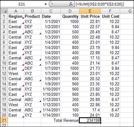
The array formulas in E22:E24 are also powerful array formulas. The formula for E22 is this:
=SUM(IF(A$2:A$19=$A22,D$2:D$19*E$2:E$19,0))
The code to enter these formulas follows. Although the formulas appear in the user interface in A1-style notation, you must use R1C1-style notation for entering array formulas:
Sub EnterArrayFormulas()
    ' Add a formula to multiply unit price x quantity
    FinalRow = Cells(Rows.Count, 1).End(xlUp).Row
    Cells(FinalRow + 1, 5).FormulaArray = "=SUM(R2C[-1]:R[-1]C[-1]*R2C:R[-1]C)"
End Sub
Tip
To quickly find the R1C1 formula, use this trick.Enter a regular A1-style formula or an array formula in any cell in Excel.Select that cell.Switch to the VBA editor.Press Ctrl+G to display the Immediate window.Type Print ActiveCell.FormulaR1C1 and press Enter.Excel will convert the formula in the formula bar to an R1C1 style formula.
Conditional formatting is one of the features that changed in Excel 2007 VBA. Read Chapter 7, “What’s New in Excel 2007 and What’s Changed,” to learn many more features that have changed significantly in Excel 2007.