
Using the arcane Advanced Filter command is so hard in the Excel user interface that it is pretty rare to find someone who enjoys using it regularly. In versions of Excel prior to 2007, the AutoFilter command was probably used by most people rather than the Advanced Filter. In Excel 2007, Microsoft renamed the AutoFilter to Filter and made advances in the types of filters possible, making the Advanced Filter a less likely choice in the user interface.
However, in VBA, advanced filters are a joy to use. With a single line of code, you can rapidly extract a subset of records from a database or quickly get a unique list of values in any column. This is critical when you want to run reports for a specific region or customer.
Because not many people use the Advanced Filter feature, I walk you through examples, using the user interface to build an advanced filter, and then show you the analogous code. You will be amazed at how complex the user interface seems and yet how easy it is to program a powerful advanced filter to extract records.
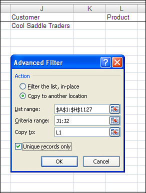
One reason why Advanced Filter is hard to use is that you can use the filter in several different ways. You must make three basic choices in the Advanced Filter dialog box. Because each choice has two options, there are eight (2 x 2 x 2) possible combinations of these choices. The three choices are shown in Figure 12.1 and described here:
Action—. You can choose Filter the List, In-Place, or Copy to Another Location. If you choose to filter the records in place, the nonmatching rows are hidden. Choosing to copy to a new location copies the records that match the filter to a new range.
Criteria—. You can filter with or without criteria. Filtering with criteria is appropriate for getting a subset of rows. Filtering without criteria is still useful when you want a subset of columns or when you are using the Unique Records Only option.
Unique—. You can choose to request Unique Records Only or all matching records. The Unique option makes the Advanced Filter command one of the fastest ways to find a unique list of values in one field.

One of the simplest uses of Advanced Filter is to extract a unique list of a single field from a dataset. In this example, you want to get a unique list of customers from a sales report. You know that customer is in Column D of the dataset. You have an unknown number of records starting in cell A2. (Row 1 is the header row.) There is nothing located to the right of the dataset.
To extract a unique list of values, follow these steps:
With the cursor anywhere in the data range, select Advanced from the Sort & Filter group on the Data ribbon. The first time that you use the Advanced Filter command on a worksheet, Excel automatically populates the List Range text box with the entire range of your dataset. On subsequent uses of the Advanced Filter command, this dialog box remembers the settings from the prior advanced filter.
Choose the Unique Records Only check box at the bottom of the dialog.
In the Action section, choose Copy to Another Location.
Type
J1in the Copy To text box.
By default, Excel copies all the columns in the dataset. You can filter just the Customer column by either limiting the List Range to include only Column D, or by specifying one or more headings in the Copy To range. Either method has its own drawbacks.
Edit the List Range to point to the Customer column. In this case, it means changing the default $A$1:$H$1127 to $D$1:$D$1127. The Advanced Filter dialog should appear.
Caution
When you initially edit any range in the dialog box, Excel might be in Point mode. In this mode, pressing a left- or right-arrow key will insert a cell reference in the text box. If you see the word Point in the lower-left corner of your Excel window, press the F2 key to change from Point mode to Edit mode.
The drawback of this method is that Excel remembers the list range on subsequent uses of the Advanced Filter command. If you later want to get a unique list of regions, you will be constantly specifying the list range.
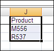
With a little forethought before invoking the Advanced Filter command, you can allow Excel to keep the default list range of $A$1:$H$1127. In cell J1, type the Customer heading. In Figure 12.2, you leave the List Range field pointing to Columns A through H. Because the Copy To range of J1 already contains a valid heading from the list range, Excel copies data only from the Customer column. I prefer this method, particularly if you will be doing multiple advanced filters. Because Excel remembers the prior settings from the last advanced filter, it is more convenient to always filter the entire columns of the list range and limit the columns by setting up headings in the Copy To range.

After using either of these methods to perform the Advanced Filter, a concise list of the unique customers appears in Column J (see Figure 12.3).

In VBA, you use the AdvancedFilter method to carry out the Advanced Filter command. Again, you have three choices to make:
Action—. Choose to either filter in place with the parameter
Action:=xlFilterInPlaceor to copy withAction:=xlFilterCopy. If you want to copy, you also have to specify the parameterCopyToRange:=Range("J1").Criteria—. To filter with criteria, include the parameter
CriteriaRange:=Range("L1:L2"). To filter without criteria, omit this optional parameter.Unique—. To return only unique records, specify the parameter
Unique:=True.
The following code sets up a single column output range two columns to the right of the last-used column in the data range:
Sub GetUniqueCustomers()
    Dim IRange As Range
    Dim ORange As Range

    ' Find the size of today's dataset
    FinalRow = Cells(Rows.Count, 1).End(xlUp).Row
    NextCol = Cells(1, Columns.Count).End(xlToLeft).Column + 2

    ' Set up output range. Copy heading from D1 there
    Range("D1").Copy Destination:=Cells(1, NextCol)
    Set ORange = Cells(1, NextCol)

    ' Define the Input Range
    Set IRange = Range("A1").Resize(FinalRow, NextCol - 2)

    ' Do the Advanced Filter to get unique list of customers
    IRange.AdvancedFilter Action:=xlFilterCopy, CopyToRange:=ORange, Unique:=True

End Sub
By default, an advanced filter copies all columns. If you just want one particular column, use that column heading as the heading in the output range.
The first bit of code finds the final row and column in the dataset. Although it is not necessary to do so, I define an object variable for the output range (ORange) and for the input range (IRange).
This code is generic enough that it will not have to be rewritten if new columns are added to the dataset at a later time. Setting up the object variables for the input and output range is done for readability instead of out of necessity. The previous code could be written just as easily like this shortened version:
Sub UniqueCustomerRedux()
    ' Copy a heading to create an output range
    Range("J1").Value = Range("D1").Value
    ' Do the Advanced Filter
    Range("A1").CurrentRegion.AdvancedFilter xlFilterCopy, _
        CopyToRange:=Range("J1"), Unique:=True
End Sub
When you run either of the previous blocks of code on the sample dataset, you get a unique list of customers off to the right of the data. In Figure 12.3, you saw the original dataset in Columns A:H and the unique customers in Column J. The key to getting a unique list of customers is copying the header from the Customer field to a blank cell and specifying this cell as the output range.
After you have the unique list of customers, you can easily sort the list and add a SUMIF formula to get total revenue by customer. The following code gets the unique list of customers, sorts it, and then builds a formula to total revenue by customer. Figure 12.4 shows the results:
Sub RevenueByCustomers()
    Dim IRange As Range
    Dim ORange As Range

    ' Find the size of today's dataset
    FinalRow = Cells(Rows.Count, 1).End(xlUp).Row
    NextCol = Cells(1, Columns.Count).End(xlToLeft).Column + 2

    ' Set up output range. Copy heading from D1 there
    Range("D1").Copy Destination:=Cells(1, NextCol)
    Set ORange = Cells(1, NextCol)

    ' Define the Input Range
    Set IRange = Range("A1").Resize(FinalRow, NextCol - 2)

    ' Do the Advanced Filter to get unique list of customers
    IRange.AdvancedFilter Action:=xlFilterCopy, _
        CopyToRange:=ORange, Unique:=True

    ' Determine how many unique customers we have
    LastRow = Cells(Rows.Count, NextCol).End(xlUp).Row

    ' Sort the data
    Cells(1, NextCol).Resize(LastRow, 1).Sort Key1:=Cells(1, NextCol), _
        Order1:=xlAscending, Header:=xlYes

    ' Add a SUMIF formula to get totals
    Cells(1, NextCol + 1).Value = "Revenue"
    Cells(2, NextCol + 1).FormulaR1C1 = "=SUM(R2C4:R" & FinalRow & "C4,RC[-1], _
        R2C6:R" & FinalRow & "C6)"
    If LastRow > 2 Then
        Cells(2, NextCol + 1).Copy Cells(3, NextCol + 1).Resize(LastRow - 2, 1)
    End If

End Sub
Another use of a unique list of values is to quickly populate a list box or a combo box on a userform. Suppose, for instance, that you have a macro that can run a report for any one specific customer. To allow your clients to choose which customers to report, create a simple userform. Add a list box to the userform and set the list box’s MultiSelect property to 1-fmMultiSelectMulti. I named my form frmReport. In addition to the list box, I have four command buttons: OK, Cancel, Mark All, Clear All. The code to run the form follows. Note the Userform_Initialize procedure includes an advanced filter to get the unique list of customers from the dataset:
Private Sub CancelButton_Click()
    Unload Me
End Sub

Private Sub cbSubAll_Click()
    For i = 0 To lbCust.ListCount - 1
        Me.lbCust.Selected(i) = True
    Next i
End Sub

Private Sub cbSubClear_Click()
    For i = 0 To lbCust.ListCount - 1
        Me.lbCust.Selected(i) = False
    Next i
End Sub

Private Sub OKButton_Click()
    For i = 0 To lbCust.ListCount - 1
        If Me.lbCust.Selected(i) = True Then
            ' Call a routine to produce this report
            RunCustReport WhichCust:=Me.lbCust.List(i)
        End If
    Next i
    Unload Me
End Sub

Private Sub UserForm_Initialize()
    Dim IRange As Range
    Dim ORange As Range

    ' Find the size of today's dataset
    FinalRow = Cells(Rows.Count, 1).End(xlUp).Row
    NextCol = Cells(1, Columns.Count).End(xlToLeft).Column + 2

    ' Set up output range. Copy heading from D1 there
    Range("D1").Copy Destination:=Cells(1, NextCol)
    Set ORange = Cells(1, NextCol)

    ' Define the Input Range
    Set IRange = Range("A1").Resize(FinalRow, NextCol - 2)

    ' Do the Advanced Filter to get unique list of customers
    IRange.AdvancedFilter Action:=xlFilterCopy, _
        CopyToRange:=ORange, Unique:=True

    ' Determine how many unique customers we have
    LastRow = Cells(Rows.Count, NextCol).End(xlUp).Row

    ' Sort the data
    Cells(1, NextCol).Resize(LastRow, 1).Sort Key1:=Cells(1, NextCol), _
        Order1:=xlAscending, Header:=xlYes

With Me.lbCust
    .RowSource = ""
    .List = Cells(2, NextCol).Resize(LastRow - 1, 1).Value
End With

    ' Erase the temporary list of customers
    Cells(1, NextCol).Resize(LastRow, 1).Clear
End Sub
Launch this form with a simple module such as this:
Sub ShowCustForm()
    frmReport.Show
End Sub
Your clients are presented with a list of all valid customers from the dataset. Because the list box’s MultiSelect property is set to allow it, they can select any number of customers, as shown in Figure 12.5.

To get all unique combinations of two (or more) fields, build the output range to include the additional fields. This code sample builds a list of unique combinations of two fields, Customer and Product:
Sub UniqueCustomerProduct()
    Dim IRange As Range
    Dim ORange As Range

    ' Find the size of today's dataset
    FinalRow = Cells(Rows.Count, 1).End(xlUp).Row
    NextCol = Cells(1, Columns.Count).End(xlToLeft).Column + 2

    ' Set up output range. Copy headings from D1 & B1
    Range("D1").Copy Destination:=Cells(1, NextCol)
    Range("B1").Copy Destination:=Cells(1, NextCol + 1)
    Set ORange = Cells(1, NextCol).Resize(1, 2)

    ' Define the Input Range
    Set IRange = Range("A1").Resize(FinalRow, NextCol - 2)

    ' Do the Advanced Filter to get unique list of customers & product
    IRange.AdvancedFilter Action:=xlFilterCopy, _
        CopyToRange:=ORange, Unique:=True

    ' Determine how many unique rows we have
    LastRow = Cells(Rows.Count, NextCol).End(xlUp).Row

    ' Sort the data
    Cells(1, NextCol).Resize(LastRow, 2).Sort Key1:=Cells(1, NextCol), _
        Order1:=xlAscending, Key2:=Cells(1, NextCol + 1), _
        Order2:=xlAscending, Header:=xlYes

End Sub
In the result shown in Figure 12.6, you can see that Enhanced Eggbeater buys only one product, and Agile Aquarium buys three products. This might be useful to use as a guide in running reports on either customer by product or product by customer.

As the name implies, Advanced Filter is usually used to filter records—in other words, to get a subset of data. You specify the subset by setting up a criteria range. Even if you are familiar with criteria, be sure to check out using the powerful Boolean formula in criteria ranges later in this chapter, in the section “The Most Complex Criteria—Replacing the List of Values with a Condition Created as the Result of a Formula.”
Set up a criteria range in a blank area of the worksheet. A criteria range always includes two or more rows. The first row of the criteria range contains one or more field header values to match the one(s) in the data range you want to filter. The second row contains a value showing what records to extract. In Figure 12.8, range J1:J2 is the criteria range, and range L1 is the output range.
In the Excel user interface, to extract a unique list of products that were purchased by a particular customer, select Advanced Filter and set up the Advanced Filter dialog as shown earlier in Figure 12.7. Figure 12.8 shows the results.

In VBA, you use the following code to perform an equivalent advanced filter:
Sub UniqueProductsOneCustomer()
    Dim IRange As Range
    Dim ORange As Range
    Dim CRange As Range

    ' Find the size of today's dataset
    FinalRow = Cells(Rows.Count, 1).End(xlUp).Row
    NextCol = Cells(1, Columns.Count).End(xlToLeft).Column + 2

    ' Set up the Output Range with one customer
    Cells(1, NextCol).Value = Range("D1").Value
    ' In reality, this value should be passed from the userform
    Cells(2, NextCol).Value = Range("D2").Value
    Set CRange = Cells(1, NextCol).Resize(2, 1)

    ' Set up output range. Copy heading from B1 there
    Range("B1").Copy Destination:=Cells(1, NextCol + 2)
    Set ORange = Cells(1, NextCol + 2)

    ' Define the Input Range
    Set IRange = Range("A1").Resize(FinalRow, NextCol - 2)

    ' Do the Advanced Filter to get unique list of customers & product
    IRange.AdvancedFilter Action:=xlFilterCopy, _
        CriteriaRange:=CRange, CopyToRange:=ORange, Unique:=True
    ' The above could also be written as:
    'IRange.AdvancedFilter xlFilterCopy, CRange, ORange, True

    ' Determine how many unique rows we have
    LastRow = Cells(Rows.Count, NextCol + 2).End(xlUp).Row

    ' Sort the data
    Cells(1, NextCol + 2).Resize(LastRow, 1).Sort Key1:=Cells(1, NextCol + 2), _
        Order1:=xlAscending, Header:=xlYes

End SubYou may want to filter records that match one criteria or another (for example, extract customers who purchased either product M556 or product R537). This is called a logical OR criteria.
When your criteria should be joined by a logical OR, place the criteria on subsequent rows of the criteria range. For example, the criteria range shown in J1:J3 of Figure 12.9 tells you which customers order product M556 or product R537.
Other times, you will want to filter records that match one criteria and another criteria. For example, you might want to extract records where the product sold was W435 and the region was the West region. This is called a logical AND.
To join two criteria by AND, put both criteria on the same row of the criteria range. For example, the criteria range shown in J1:K2 of Figure 12.10 gets the customers who ordered product W435 in the West region.

The criteria range shown in Figure 12.11 is based on two different fields. They are joined with an OR. The query finds all records from either the West region or records where the product is W435.

It is possible to have a criteria range with multiple logical AND and logical OR criteria joined together. Although this might work in some situations, in other scenarios it quickly gets out of hand. Luckily, Excel allows for criteria where the records are selected as the result of a formula to handle this situation.
Working with Very Complex Criteria
Your clients so loved the “Create a Customer” report, they hired you to write a new report. In this case, they could select any customer, any product, any region, or any combination of them. You can quickly adapt the frmReport userform to show three list boxes, as shown in Figure 12.12.

In your first test, imagine that you select two customers and two products. In this case, your program has to build a five-row criteria range, as shown in Figure 12.13. This isn’t too bad.

This gets crazy if someone selects 10 products, all regions but the house region, and all customers except the internal customer. Your criteria range would need unique combinations of the selected fields. This could easily be 10 products times 9 regions times 499 customers, or more than 44,000 rows of criteria range. You can quickly end up with a criteria range that spans thousands of rows and three columns. I was once foolish enough to actually try running an advanced filter with such a criteria range. It would still be trying to compute if I hadn’t rebooted the computer.
The solution for this report is to replace the lists of values with a formula-based condition.
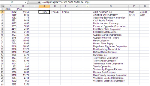
Amazingly, there is an incredibly obscure version of Advanced Filter criteria that can replace the 44,000-row criteria range in the case study. In the alternative form of criteria range, the top row is left blank. There is no heading above the criteria. The criteria set up in Row 2 are a formula that results in True or False. If the formula contains any relative references to Row 2 of the input range, Excel compares that formula to every row of the input range, one by one.
For example, if we want all records where the Gross Profit Percentage is below 53%, the formula built in J2 would reference the Profit in H2 and the Revenue in F2. We would leave J1 blank to tell Excel that we are using a formula-based criterion. Cell J2 would contain the formula =(H2/F2)<0.53. The criteria range for the advanced filter would be specified as J1:J2.
As Excel performs the advanced filter, it logically copies the formula and applies it to all rows in the database. Anywhere that the formula evaluates to True, the record is included in the output range.
This is incredibly powerful and runs remarkably quickly. You can combine multiple formulas in adjacent columns or rows to join the formula criteria with AND or OR, just as you do with regular criteria.
The following is the code for this new userform. Note the logic in OKButton_Click that builds the formula. Figure 12.14 shows the Excel sheet just before the Advanced Filter is run:
Private Sub CancelButton_Click()
    Unload Me
End Sub

Private Sub cbSubAll_Click()
    For i = 0 To lbCust.ListCount - 1
        Me.lbCust.Selected(i) = True
    Next i
End Sub

Private Sub cbSubClear_Click()
    For i = 0 To lbCust.ListCount - 1
        Me.lbCust.Selected(i) = False
    Next i
End Sub

Private Sub CommandButton1_Click()
    ' Clear all products
    For i = 0 To lbProduct.ListCount - 1
        Me.lbProduct.Selected(i) = False
    Next i
End Sub

Private Sub CommandButton2_Click()
    ' Mark all products
    For i = 0 To lbProduct.ListCount - 1
        Me.lbProduct.Selected(i) = True
    Next i
End Sub

Private Sub CommandButton3_Click()
    ' Clear all regions
    For i = 0 To lbRegion.ListCount - 1
        Me.lbRegion.Selected(i) = False
    Next i
End Sub

Private Sub CommandButton4_Click()
    ' Mark all regions
    For i = 0 To lbRegion.ListCount - 1
        Me.lbRegion.Selected(i) = True
    Next i
End Sub

Private Sub OKButton_Click()
    Dim CRange As Range, IRange As Range, ORange As Range
    ' Build a complex criteria that ANDS all choices together
    NextCCol = 10
    NextTCol = 15

    For j = 1 To 3
        Select Case j
            Case 1
                MyControl = "lbCust"
                MyColumn = 4
            Case 2
                MyControl = "lbProduct"
                MyColumn = 2
            Case 3
                MyControl = "lbRegion"
                MyColumn = 1
        End Select
        NextRow = 2
        ' Check to see what was selected.
        For i = 0 To Me.Controls(MyControl).ListCount - 1
            If Me.Controls(MyControl).Selected(i) = True Then
                Cells(NextRow, NextTCol).Value = _
                    Me.Controls(MyControl).List(i)
                NextRow = NextRow + 1
            End If
        Next i
        ' If anything was selected, build a new criteria formula
        If NextRow > 2 Then
            ' the reference to Row 2 must be relative in order to work
            MyFormula = "=NOT(ISNA(MATCH(RC" & MyColumn & ",R2C" & NextTCol & _
                ":R" & NextRow - 1 & "C" & NextTCol & ",False)))"
            Cells(2, NextCCol).FormulaR1C1 = MyFormula
            NextTCol = NextTCol + 1
            NextCCol = NextCCol + 1
        End If
    Next j
    Unload Me

    ' Figure 12.14 shows the worksheet at this point
    ' if we built any criteria, define the criteria range
    If NextCCol > 10 Then
        Set CRange = Range(Cells(1, 10), Cells(2, NextCCol - 1))
        Set IRange = Range("A1").CurrentRegion
        Set ORange = Cells(1, 20)
        IRange.AdvancedFilter xlFilterCopy, CRange, ORange

        ' Clear out the criteria
        Cells(1, 10).Resize(1, 10).EntireColumn.Clear
    End If

    ' At this point, the matching records are in T1

End Sub

Private Sub UserForm_Initialize()
    Dim IRange As Range
    Dim ORange As Range

    ' Find the size of today's dataset
    FinalRow = Cells(Rows.Count, 1).End(xlUp).Row
    NextCol = Cells(1, Columns.Count).End(xlToLeft).Column + 2

    ' Define the input range
    Set IRange = Range("A1").Resize(FinalRow, NextCol - 2)

    ' Set up output range for Customer. Copy heading from D1 there
    Range("D1").Copy Destination:=Cells(1, NextCol)
    Set ORange = Cells(1, NextCol)

    ' Do the Advanced Filter to get unique list of customers
    IRange.AdvancedFilter Action:=xlFilterCopy, CriteriaRange:="", _
        CopyToRange:=ORange, Unique:=True

    ' Determine how many unique customers we have
    LastRow = Cells(Rows.Count, NextCol).End(xlUp).Row

    ' Sort the data
    Cells(1, NextCol).Resize(LastRow, 1).Sort Key1:=Cells(1, NextCol), _
        Order1:=xlAscending, Header:=xlYes

    With Me.lbCust
        .RowSource = ""
        FinalRow = Cells(Rows.Count, 10).End(xlUp).Row
        For Each cell In Cells(2, NextCol).Resize(LastRow - 1, 1)
            .AddItem cell.Value
        Next cell
    End With

    ' Erase the temporary list of customers
    Cells(1, NextCol).Resize(LastRow, 1).Clear

    ' Set up output range for product. Copy heading from D1 there
    Range("B1").Copy Destination:=Cells(1, NextCol)
    Set ORange = Cells(1, NextCol)

    ' Do the Advanced Filter to get unique list of customers
    IRange.AdvancedFilter Action:=xlFilterCopy, _
        CopyToRange:=ORange, Unique:=True

    ' Determine how many unique customers we have
    LastRow = Cells(Rows.Count, NextCol).End(xlUp).Row

    ' Sort the data
    Cells(1, NextCol).Resize(LastRow, 1).Sort Key1:=Cells(1, NextCol), _
        Order1:=xlAscending, Header:=xlYes

    With Me.lbProduct
        .RowSource = ""
        FinalRow = Cells(Rows.Count, 10).End(xlUp).Row
        For Each cell In Cells(2, NextCol).Resize(LastRow - 1, 1)
            .AddItem cell.Value
        Next cell
    End With

    ' Erase the temporary list of customers
    Cells(1, NextCol).Resize(LastRow, 1).Clear

    ' Set up output range for Region. Copy heading from A1 there
    Range("A1").Copy Destination:=Cells(1, NextCol)
    Set ORange = Cells(1, NextCol)

    ' Do the Advanced Filter to get unique list of customers
    ' Figure 12.15 shows the worksheet state just before this line
    IRange.AdvancedFilter Action:=xlFilterCopy, CopyToRange:=ORange, _
        Unique:=True

    ' Determine how many unique customers we have
    LastRow = Cells(Rows.Count, NextCol).End(xlUp).Row

    ' Sort the data
    Cells(1, NextCol).Resize(LastRow, 1).Sort Key1:=Cells(1, NextCol), _
        Order1:=xlAscending, Header:=xlYes

    With Me.lbRegion
        .RowSource = ""
        FinalRow = Cells(Rows.Count, 10).End(xlUp).Row
        For Each cell In Cells(2, NextCol).Resize(LastRow - 1, 1)
            .AddItem cell.Value
        Next cell
    End With

    ' Erase the temporary list of customers
    Cells(1, NextCol).Resize(LastRow, 1).Clear

End Sub
Figure 12.14 shows the worksheet just before the AdvancedFilter method is called. The user has selected customers, products, and regions. The macro has built temporary tables in Columns O, P, Q to show which values the user selected. The criteria range is J1:L2. That criteria formula in J2 looks to see whether the value in $D2 is in the list of selected customers in O. The formulas in K2 and L2 compare $B2 to Column P and $A2 to Column Q.
Caution
Excel VBA Help says that if you do not specify a criteria range, no criteria is used. This is not true in Excel 2007—if no criteria range is specified, the advanced filter inherits the criteria range from the prior advanced filter. You should include CriteriaRange:="" to clear the prior value.
The formula-based conditions formula criteria are cool, but are a rarely used feature in a rarely used function. Some interesting business applications use this technique. For example, this criteria formula would find all the above-average rows in the dataset:
=$A2>Average($A$2:$A$60000)
It is possible to filter a large dataset in place. In this case, you do not need an output range. You would normally specify criteria range—otherwise you return 100% of the records and there is no need to do the advanced filter!
In the user interface of Excel, running a Filter in Place makes sense: You can easily peruse the filtered list looking for something in particular.
Running a Filter in Place in VBA is a little less convenient. The only good way to programmatically peruse through the filtered records is to use the xlCellTypeVisible option of the SpecialCells method. In the Excel user interface, the equivalent action is to select Find & Select, Go to Special from the Home ribbon. In the Go to Special dialog, select Visible Cells Only, as shown in Figure 12.15.

To run a Filter in Place, use the constant XLFilterInPlace as the Action parameter in the AdvancedFilter command and remove the CopyToRange from the command:
IRange.AdvancedFilter Action:=xlFilterInPlace, CriteriaRange:=CRange, _
    Unique:=False
Then, the programmatic equivalent to loop through Visible Cells Only is this code:
For Each cell In Range("A2:A" & FinalRow).SpecialCells(xlCellTypeVisible)
    Ctr = Ctr + 1
Next cell
MsgBox Ctr & " cells match the criteria"Just as when using Copy, you have to watch out for the possibility of having no records match the criteria. In this case, however, it is more difficult to realize that nothing is returned. You generally find out when the .SpecialCells method returns a runtime error 1004—no cells were found.
To catch this condition, you have to set up an error trap to anticipate the 1004 error with the SpecialCells method. (See Chapter 25, “Handling Errors,” for more information on catching errors.)
    On Error GoTo NoRecs
    For Each cell In Range("A2:A" & FinalRow).SpecialCells(xlCellTypeVisible)
        Ctr = Ctr + 1
    Next cell
    On Error GoTo 0
    MsgBox Ctr & " cells match the criteria"
    Exit Sub
NoRecs:
    MsgBox "No records match the criteria"
End Sub
This error trap works because I specifically exclude the header row from the SpecialCells range. The header row is always visible after an advanced filter. Including it in the range would prevent the 1004 error from being raised.
After doing a Filter in Place, you can get all records to show again by using the ShowAllData method:
ActiveSheet.ShowAllData
It is possible to use Filter in Place and Unique Records Only. However, when you specified an output range of only Product and Customer, the advanced filter was able to give you only the unique combinations of Customer and Product. If you ask for unique records from a dataset with 10 fields, the only records that will not be shown are those records where all 10 fields are exact duplicates.
The examples at the beginning of this chapter talked about using xlFilterCopy to get a unique list of values in a field. We used unique lists of customer, region, and product to populate the list boxes in our report-specific userforms.
A more common scenario, however, is to use an advanced filter to return all records that match the criteria. After the client selects which customer to report, an advanced filter can extract all records for that customer.
In all the examples in the following sections, you want to leave the Unique Records Only check box unselected. You do this in VBA by specifying Unique:=False as a parameter to the AdvancedFilter method.
This is easy to do, and you have some powerful options. If you need only a subset of fields for a report, copy only those field headings to the output range. If you want to resequence the fields to appear exactly as you need them in the report, you can do this by changing the sequence of the headings in the output range.
I walk you through three quick examples to show the options available.
To copy all columns, specify a single blank cell as the output range. You will get all columns for those records that match the criteria as shown in Figure 12.16:
Sub AllColumnsOneCustomer()
    Dim IRange As Range
    Dim ORange As Range
    Dim CRange As Range

    ' Find the size of today's dataset
    FinalRow = Cells(Rows.Count, 1).End(xlUp).Row
    NextCol = Cells(1, Columns.Count).End(xlToLeft).Column + 2

    ' Set up the criteria range with one customer
    Cells(1, NextCol).Value = Range("D1").Value
    ' In reality, this value should be passed from the userform
    Cells(2, NextCol).Value = Range("D2").Value
    Set CRange = Cells(1, NextCol).Resize(2, 1)

    ' Set up output range. It is a single blank cell
    Set ORange = Cells(1, NextCol + 2)

    ' Define the Input Range
    Set IRange = Range("A1").Resize(FinalRow, NextCol - 2)

    ' Do the Advanced Filter to get unique list of customers & product
    IRange.AdvancedFilter Action:=xlFilterCopy, _
        CriteriaRange:=CRange, CopyToRange:=ORange


End Sub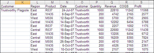
If you are doing the advanced filter to send records to a report, it is likely that you might only need a subset of columns and you might need them in a different sequence.
Here is an example that will finish off the frmReport example from earlier in the chapter. As you remember, frmReport would allow the client to select a customer. The OK button would then call the RunCustReport routine, passing a parameter to identify for which customer to prepare a report.
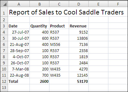
Imagine this is a report being sent to the customer. The customer really doesn’t care about the surrounding region, and we definitely do not want to reveal our cost of goods sold or profit. Assuming that we will put the customer in the title of the report, the fields that we really need to produce the report are Date, Quantity, Product, Revenue.
The following code copies those headings to the output range. The advanced filter produces data, as shown in Figure 12.17. The program then goes on to copy the matching records to a new workbook. A title and total row is added, and the report is saved with the customer’s name. Figure 12.18 shows the final report.
Sub RunCustReport(WhichCust As Variant)
    Dim IRange As Range
    Dim ORange As Range
    Dim CRange As Range
    Dim WBN As Workbook
    Dim WSN As Worksheet
    Dim WSO As Worksheet

    Set WSO = ActiveSheet
    ' Find the size of today's dataset
    FinalRow = Cells(Rows.Count, 1).End(xlUp).Row
    NextCol = Cells(1, Columns.Count).End(xlToLeft).Column + 2

    ' Set up the criteria range with one customer
    Cells(1, NextCol).Value = Range("D1").Value
    Cells(2, NextCol).Value = WhichCust
    Set CRange = Cells(1, NextCol).Resize(2, 1)

    ' Set up output range. We want Date, Quantity, Product, Revenue
    ' These columns are in C, E, B, and F
    Cells(1, NextCol + 2).Resize(1, 4).Value = _
        Array(Cells(1, 3), Cells(1, 5), Cells(1, 2), Cells(1, 6))
    Set ORange = Cells(1, NextCol + 2).Resize(1, 4)

    ' Define the Input Range
    Set IRange = Range("A1").Resize(FinalRow, NextCol - 2)

    ' Do the Advanced Filter to get unique list of customers & products
    IRange.AdvancedFilter Action:=xlFilterCopy, _
        CriteriaRange:=CRange, CopyToRange:=ORange

    ' At this point, the data looks like Figure 12.18

    ' Create a new workbook with one blank sheet to hold the output
    Set WBN = Workbooks.Add(xlWBATWorksheet)
    Set WSN = WBN.Worksheets(1)

    ' Set up a title on WSN
    WSN.Cells(1, 1).Value = "Report of Sales to " & WhichCust

    ' Copy data from WSO to WSN
    WSO.Cells(1, NextCol + 2).CurrentRegion.Copy Destination:=WSN.Cells(3, 1)
    TotalRow = WSN.Cells(Rows.Count, 1).End(xlUp).Row + 1
    WSN.Cells(TotalRow, 1).Value = "Total"
    WSN.Cells(TotalRow, 2).FormulaR1C1 = "=SUM(R2C:R[-1]C)"
    WSN.Cells(TotalRow, 4).FormulaR1C1 = "=SUM(R2C:R[-1]C)"

    ' Format the new report with bold
    WSN.Cells(3, 1).Resize(1, 4).Font.Bold = True
    WSN.Cells(TotalRow, 1).Resize(1, 4).Font.Bold = True
    WSN.Cells(1, 1).Font.Size = 18

    WBN.SaveAs "C:" & WhichCust & ".xls"
    WBN.Close SaveChanges:=False

    WSO.Select

    ' clear the output range, etc.
    Range("J1:Z1").EntireColumn.Clear

End Sub
Utilizing Two Kinds of Advanced Filters to Create a Report for Each Customer
The final advanced filter example for this chapter uses several advanced filter techniques. Let’s say that after importing invoice records, you want to send a purchase summary to each customer. The process would be as follows:
Run an advanced filter requesting unique values to get a list of customers in J. This
AdvancedFilterwould specify theUnique:=Trueparameter and use aCopyToRangethat includes a single heading for Customer:' Set up output range. Copy heading from D1 there Range("D1").Copy Destination:=Cells(1, NextCol) Set ORange = Cells(1, NextCol) ' Define the Input Range Set IRange = Range("A1").Resize(FinalRow, NextCol - 2) ' Do the Advanced Filter to get unique list of customers IRange.AdvancedFilter Action:=xlFilterCopy, CriteriaRange:="", _ CopyToRange:=ORange, Unique:=TrueFor each customer in the list of unique customers in Column J, perform steps 3 through 7. Find the number of customers in the output range from step 1. Then, use a
For Each Cellloop to loop through the customers:' Loop through each customer FinalCust = Cells(Rows.Count, NextCol).End(xlUp).Row For Each cell In Cells(2, NextCol).Resize(FinalCust - 1, 1) ThisCust = cell.Value ' ... Steps 3 through 7 here Next CellBuild a criteria range in L1:L2 to be used in a new advanced filter. The criteria range would include a heading of Customer in L1 and the customer name from this iteration of the loop in cell L2:
' Set up the Criteria Range with one customer
Cells(1, NextCol + 2).Value = Range("D1").Value
Cells(2, NextCol + 2).Value = ThisCust
Set CRange = Cells(1, NextCol + 2).Resize(2, 1)
Do an advanced filter to copy matching records for this customer to Column N. This
Advanced Filterstatement would specify theUnique:=Falseparameter. Because we want only the columns for Date, Quantity, Product, and Revenue, theCopyToRangespecifies a four-column range with those headings copied in the proper order:' Set up output range. We want Date, Quantity, Product, Revenue ' These columns are in C, E, B, and F Cells(1, NextCol + 4).Resize(1, 4).Value = _ Array(Cells(1, 3), Cells(1, 5), Cells(1, 2), Cells(1, 6)) Set ORange = Cells(1, NextCol + 4).Resize(1, 4) ' Do the Advanced Filter to get unique list of customers & product IRange.AdvancedFilter Action:=xlFilterCopy, CriteriaRange:=CRange, _ CopyToRange:=OrangeCopy the customer records to a report sheet in a new workbook. The VBA code uses the
Workbooks.Addmethod to create a new blank workbook. The extracted records from step 4 are copied to cell A3 of the new workbook:' Create a new workbook with one blank sheet to hold the output Set WBN = Workbooks.Add(xlWBATWorksheet) Set WSN = WBN.Worksheets(1) ' Copy data from WSO to WSN WSO.Cells(1, NextCol + 4).CurrentRegion.Copy _ Destination:=WSN.Cells(3, 1)Format the report with a title and totals. In VBA, add a title that reflects the customer’s name in cell A1. Make the headings bold and add a total below the final row:
' Set up a title on WSN
WSN.Cells(1, 1).Value = "Report of Sales to " & ThisCust

TotalRow = WSN.Cells(Rows.Count, 1).End(xlUp).Row + 1
WSN.Cells(TotalRow, 1).Value = "Total"
WSN.Cells(TotalRow, 2).FormulaR1C1 = "=SUM(R2C:R[-1]C)"
WSN.Cells(TotalRow, 4).FormulaR1C1 = "=SUM(R2C:R[-1]C)"

' Format the new report with bold
WSN.Cells(3, 1).Resize(1, 4).Font.Bold = True
WSN.Cells(TotalRow, 1).Resize(1, 4).Font.Bold = True
WSN.Cells(1, 1).Font.Size = 18
Use
SaveAsto save the workbook based on customer name. After the workbook is saved, close the new workbook. Return to the original workbook and clear the output range to prepare for the next pass through the loop:WBN.SaveAs "C:Reports" & ThisCust & ".xls" WBN.Close SaveChanges:=False WSO.Select Set WSN = Nothing Set WBN = Nothing ' clear the output range, etc. Cells(1, NextCol + 2).Resize(1, 10).EntireColumn.Clear
The complete code is as follows:
Sub RunReportForEachCustomer()
    Dim IRange As Range
    Dim ORange As Range
    Dim CRange As Range
    Dim WBN As Workbook
    Dim WSN As Worksheet
    Dim WSO As Worksheet

    Set WSO = ActiveSheet
    ' Find the size of today's dataset
    FinalRow = Cells(Rows.Count, 1).End(xlUp).Row
    NextCol = Cells(1, Columns.Count).End(xlToLeft).Column + 2

    ' First - get a unique list of customers in J
    ' Set up output range. Copy heading from D1 there
    Range("D1").Copy Destination:=Cells(1, NextCol)
    Set ORange = Cells(1, NextCol)

    ' Define the Input Range
    Set IRange = Range("A1").Resize(FinalRow, NextCol - 2)

    ' Do the Advanced Filter to get unique list of customers
    IRange.AdvancedFilter Action:=xlFilterCopy, CriteriaRange:="", _
        CopyToRange:=ORange, Unique:=True

    ' Loop through each customer
    FinalCust = Cells(Rows.Count, NextCol).End(xlUp).Row
    For Each cell In Cells(2, NextCol).Resize(FinalCust - 1, 1)
        ThisCust = cell.Value

        ' Set up the Criteria Range with one customer
        Cells(1, NextCol + 2).Value = Range("D1").Value
        Cells(2, NextCol + 2).Value = ThisCust
        Set CRange = Cells(1, NextCol + 2).Resize(2, 1)

        ' Set up output range. We want Date, Quantity, Product, Revenue
        ' These columns are in C, E, B, and F
        Cells(1, NextCol + 4).Resize(1, 4).Value = _
            Array(Cells(1, 3), Cells(1, 5), Cells(1, 2), Cells(1, 6))
        Set ORange = Cells(1, NextCol + 4).Resize(1, 4)

        ' Do the Advanced Filter to get unique list of customers & product
        IRange.AdvancedFilter Action:=xlFilterCopy, CriteriaRange:=CRange, _
            CopyToRange:=ORange

        ' Create a new workbook with one blank sheet to hold the output
        Set WBN = Workbooks.Add(xlWBATWorksheet)
        Set WSN = WBN.Worksheets(1)

        ' Copy data from WSO to WSN
        WSO.Cells(1, NextCol + 4).CurrentRegion.Copy _
            Destination:=WSN.Cells(3, 1)

        ' Set up a title on WSN
        WSN.Cells(1, 1).Value = "Report of Sales to " & ThisCust

        TotalRow = WSN.Cells(Rows.Count, 1).End(xlUp).Row + 1
        WSN.Cells(TotalRow, 1).Value = "Total"
        WSN.Cells(TotalRow, 2).FormulaR1C1 = "=SUM(R2C:R[-1]C)"
        WSN.Cells(TotalRow, 4).FormulaR1C1 = "=SUM(R2C:R[-1]C)"

        ' Format the new report with bold
        WSN.Cells(3, 1).Resize(1, 4).Font.Bold = True
        WSN.Cells(TotalRow, 1).Resize(1, 4).Font.Bold = True
        WSN.Cells(1, 1).Font.Size = 18

        WBN.SaveAs "C:Reports" & ThisCust & ".xlsx"
        WBN.Close SaveChanges:=False

        WSO.Select
        Set WSN = Nothing
        Set WBN = Nothing

        ' clear the output range, etc.
        Cells(1, NextCol + 2).Resize(1, 10).EntireColumn.Clear
    Next cell

    Cells(1, NextCol).EntireColumn.Clear
    MsgBox FinalCust - 1 & " Reports have been created!"
End Sub
This is a remarkable 75 lines of code. Incorporating a couple of advanced filters and not much else, we’ve managed to produce a tool that created 27 reports in less than 1 minute (see Figure 12.19). Even an Excel power user would normally take 2 to 3 minutes per report to create these manually. In less than 60 seconds, this code easily will save someone a few hours every time these reports need to be created. Imagine the real scenario where there are hundreds of customers. I guarantee that there are people in every city who are manually creating these reports in Excel because they simply don’t realize the power of Excel VBA.

The AutoFilter feature was added to Excel because people found advanced filters too hard. They are cool when used in the Excel user interface. I rarely had an occasion to use them in Excel VBA.
In Excel 2007, Microsoft renamed AutoFilter to Filter and added several dynamic new filters. These filters allow you to choose records with dates that fall in the last quarter, next week, or this year. Although the Excel user interface refers to them as filters, the VBA code still uses the term AutoFilter when referring to these filters.
The nature of the AutoFilter is that Excel will always filter in place. Thus, you have to use the SpecialCells(xlCellTypeVisible) method to access the rows returned from the filter.
There can be only one autofiltered dataset on each worksheet. To turn on the AutoFilter, you apply the AutoFilter method to any one cell in your dataset. For example, the following code turns on the AutoFilter drop-downs:
Range("A1").AutoFilterThe AutoFilter method is a toggle. If the AutoFilter drop-downs are already enabled, running the previous code will turn off the AutoFilter drop-downs. Excel 2007 adds a new FilterMode property, but it is only set to True if someone has selected a value from one of the AutoFilter drop-downs. Therefore, to figure out whether the AutoFilter is already enabled, you could the following macros to turn on/off the AutoFilter drop-downs:
Sub TurnOnAutoFilter()
    ' Turn on AutoFilters
    Worksheets("SalesReport").Select
    On Error Resume Next
    x = ActiveSheet.AutoFilter.Range.Areas.Count
    If Err.Number > 0 Then
        ActiveSheet.Range("A1").AutoFilter
    End If
    On Error Resume Next
End Sub
Use this code to turn off the AutoFilter drop-downs:
Sub TurnOffAutoFilter()
    ' Turn off AutoFilters
    Worksheets("SalesReport").Select
    On Error Resume Next
    x = ActiveSheet.AutoFilter.Range.Areas.Count
    If Err.Number = 0 Then
        ActiveSheet.Range("A1").AutoFilter
    End If
    On Error Resume Next
End SubOne cool feature is available only in Excel VBA. When you AutoFilter a list in the Excel user interface, every column in the dataset gets a field drop-down in the heading row. Sometimes you have a field that doesn’t make a lot of sense to AutoFilter. For example, in our current dataset, you might want to provide AutoFilter drop-downs for Region, Product, Customer, but not the numeric or date fields. After setting up the AutoFilter, you need one line of code to turn off each drop-down that you do not want to appear. The following code turns off the drop-downs for Columns C, E, F, G, and H:
Sub AutoFilterCustom()
    Range("A1").AutoFilter Field:=3, VisibleDropDown:=False
    Range("A1").AutoFilter Field:=5, VisibleDropDown:=False
    Range("A1").AutoFilter Field:=6, VisibleDropDown:=False
    Range("A1").AutoFilter Field:=7, VisibleDropDown:=False
    Range("A1").AutoFilter Field:=8, VisibleDropDown:=False
End Sub
I think using this tool is a fairly rare treat. Most of the time, Excel VBA lets us do things that are possible in the user interface (although it lets us do them very rapidly). The VisibleDropDown parameter actually allows us to do something in VBA that is generally not available in the Excel user interface. Your knowledgeable clients will be scratching their heads trying to figure out how you set up the cool AutoFilter with only a few filterable columns (see Figure 12.20).

In the earliest incarnation of AutoFilters, you would specify a column number, a criteria, an operator, and a second criteria. Because AutoFilters were limited to two conditions, this handled any possible filtering scenario.
For example, the following code filters to show records for the Agile Aquarium customer. As Customer is the fourth column in the dataset, the Field number is 4:
Sub SimpleFilter()
    Worksheets("SalesReport").Select
    Range("A1").AutoFilter
    Range("A1").AutoFilter Field:=4, _
        Criteria1:="=Agile Aquarium Inc."
End Sub
To clear the filter from the customer column, you use this code:
Sub SimpleFilter()
    Worksheets("SalesReport").Select
    Range("A1").AutoFilter
    Range("A1").AutoFilter Field:=4
End Sub
In previous versions of Excel, you could join two criteria with OR or AND operators. The following code would filter the customer column to one of two customers, joined by the OR operator:
Sub SimpleOrFilter()
    Worksheets("SalesReport").Select
    Range("A1").AutoFilter
    Range("A1").AutoFilter Field:=4, _
        Criteria1:="=Agile Aquarium Inc.", _
        Operator:=xlOr, Criteria2:="=Amazing Shoe Company"
End Sub
The following code returns all customers that started with the letters A through E:
Sub SimpleAndFilter()
    Worksheets("SalesReport").Select
    Range("A1").AutoFilter
    Range("A1").AutoFilter Field:=4, _
        Criteria1:=">=A", _
        Operator:=xlAnd, Criteria2:="<=EZZ"
End Sub
As the AutoFilter command became more flexible, Microsoft continued to use the same three parameters, even if they didn’t quite make sense. For example, Excel will let you filter a field by asking for the top five items or the bottom 8% of records. To use this type of filter, you specify either "5" or "8" as the Criteria1 argument, and then specify xlTop10Items, xlTop10Percent, xlBottom10Items, xlBottom10Percent as the operator. The following code produces the top 10 revenue records:
Sub Top10Filter()
    ' Top 12 Revenue Records
    Worksheets("SalesReport").Select
    Range("A1").AutoFilter
    Range("A1").AutoFilter Field:=6, _
        Criteria1:="12", _
        Operator:=xlTop10Items
End Sub
Excel 2007 offers several new filter options. Excel continues to force these filter options to fit in the old object model where the filter command must fit in an operator and up to two criteria fields.
If you specify three or more items from a filter drop-down, Excel VBA uses the xlFilterValues operator and specifies the complete list of selected items in an array passed to Criteria1. The following code selects five specific customers from the drop-down in D1:
Sub MultiSelectFilter()
    ' Select many customers
    Worksheets("SalesReport").Select
    Range("A1").AutoFilter
    Range("A1").AutoFilter Field:=4, _
        Criteria1:=Array( _
            "Amazing Shoe Company", "Cool Saddle Traders", _
            "Enhanced Eggbeater Corporation", _
            "First-Rate Notebook Inc.", "Handy Juicer Inc."), _
        Operator:=xlFilterValues
End SubPerhaps the most powerful feature in Excel 2007 filters is the new dynamic filters. These filters enable you to choose records that are above average or with a date field to select virtual periods such as Next Week or Last Year.
To use a dynamic filter, specify xlFilterDynamic as the operator and then use one of 34 values as Criteria1.
The following code finds all dates that are in next year:
Sub DynamicAutoFilter()
    Worksheets("SalesReport").Select
    Range("A1").AutoFilter
    Range("A1").AutoFilter Field:=3, _
        Criteria1:=xlFilterNextYear, _
        Operator:=xlFilterDynamic
End Sub
The following lists all the dynamic filter criteria options. Specify these values as Criteria1 in the AutoFilter method:
Criteria for values—. Use
xlFilterAboveAverageorxlFilterBelowAverageto find all the rows that are above or below average. Note that in Lake Wobegon, usingxlFilterBelowAveragewill likely return no records.Criteria for future periods—. Use
xlFilterTomorrow,xlFilterNextWeek,xlFilterNextMonth,xlFilterNextQuarter, orxlFilterNextYearto find rows that fall in a certain future period. Note that next week starts on Sunday and ends on Saturday.Criteria for current periods—. Use
xlFilterToday,xlFilterThisWeek,xlFilterThisMonth,xlFilterThisQuarter, orxlFilterThisYearto find rows that fall within the current period. Excel will use the system clock to find the current day.Criteria for past periods—. Use
xlFilterYesterday,xlFilterLastWeek,xlFilterLastMonth,xlFilterLastQuarter,xlFilterLastYear, orxlFilterYearToDateto find rows that fell within a previous period.Criteria for specific quarters—. Use
xlFilterDatesInPeriodQuarter1,xlFilterDatesInPeriodQuarter2,xlFilterDatesInPeriodQuarter3, orxlFilterDatesInPeriodQuarter4to filter to rows that fall within a specific quarter. Note that these filters do not differentiate based on a year. If you ask for quarter 1, you might get records from this January, last February, and next March.Criteria for specific months—. Use
xlFilterDatesInPeriodJanuarythroughxlFitlerDatesInPeriodDecemberto filter to records that fall during a certain month. Like the quarters, the filter does not filter to any particular year.
Unfortunately, you cannot combine criteria. You might think that you could specify xlFilterDatesInPeriodJanuary as Criteria1 and xlFilterDatesNextYear as Criteria2. Although this is a brilliant thought, Microsoft doesn’t support this syntax (yet).
Another new feature in Excel 2007 is the ability to filter based on font color, cell fill color, or conditional formatting icon.
If you are expecting the dataset to have an icon set applied, you can filter to show only records with one particular icon by using the xlFilterIcon operator.
For the criteria, you have to know which icon set has been applied and which icon within the set. The icon sets are identified using the names shown in Column A of Figure 12.21. The items range from 1 through 5. The following code filters the Revenue column to show the rows containing an upward-pointing arrow in the 5 Arrows Gray icon set:
Sub FilterByIcon()
    Worksheets("SalesReport").Select
    Range("A1").AutoFilter
    Range("A1").AutoFilter Field:=6, _
        Criteria1:=ActiveWorkbook.IconSets(xl5ArrowsGray).Item(5), _
        Operator:=xlFilterIcon
End Sub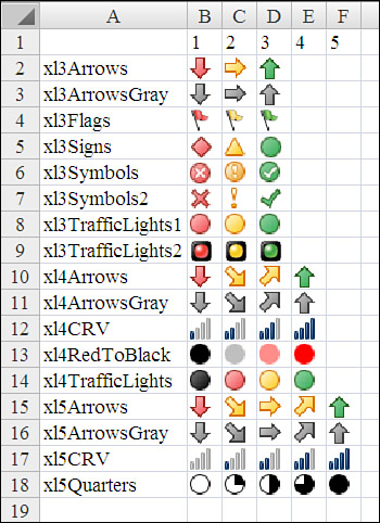
To find records that have no conditional formatting icon, use an operator of xlFilterNoIcon and do not specify any criteria.
To find records that have a particular fill color, use an operator of xlFilterCellColor and specify a particular RGB value as the criteria. This code finds all red cells in Column F:
Sub FilterByFillColor()
    Worksheets("SalesReport").Select
    Range("A1").AutoFilter
    Range("A1").AutoFilter Field:=6, _
        Criteria1:=RGB(255, 0, 0), Operator:=xlFilterCellColor
End Sub
To find records that have no fill color, use an operator of xlFilterNoFill and do not specify any criteria.
To find records that have a particular font color, use an operator of xlFilterFontColor and specify a particular RGB value as the criteria. This code finds all cells with a red font in Column F:
Sub FilterByFontColor()
    Worksheets("SalesReport").Select
    Range("A1").AutoFilter
    Range("A1").AutoFilter Field:=6, _
        Criteria1:=RGB(255, 0, 0), Operator:=xlFilterFontColor
End Sub
To find records that have no particular font color, use an operator of xlFilterAutomaticFillColor and do not specify any criteria.
Using techniques from this chapter, you have many reporting techniques available to you by using the arcane Advanced Filter tool. Chapter 13, “Using VBA to Create Pivot Tables,” introduces the most powerful feature in Excel: the pivot table. The combination of Advanced Filter and pivot tables creates reporting tools that enable amazing applications.