
Pivot tables are the most powerful tools that Excel has to offer. The concept was first put into practice by Lotus with its Improv product.
I love pivot tables because they are a really fast way to summarize massive amounts of data. You can use the basic vanilla pivot table to produce a concise summary in seconds. However, pivot tables come in so many flavors that they can be the tools of choice for many different uses. You can build pivot tables to act as the calculation engine to produce reports by store, by style, or to quickly find the top 5 or bottom 10 of anything.
I am not suggesting you use VBA to build pivot tables to give to your user. I am suggesting you use pivot tables as a means to an end—use a pivot table to extract a summary of data, and then take this summary on to better uses.
Pivot tables have been evolving. They were introduced in Excel 5 and perfected in Excel 97. In Excel 2000, pivot table creation in VBA was dramatically altered. Some new parameters were added in Excel 2002. A few new properties such as PivotFilters and TableStyle2 were added in Excel 2007. Therefore, you need to be extremely careful when writing code in Excel 2007 that might be run in Excel 2003 or Excel 2000 or Excel 97.
Just a few simple tweaks make 2003 code run in 2000, but a major overhaul is required to make any code run in Excel 97. Because it has been 10 years since the release of Excel 97 (and because Microsoft has not supported that product for 5+ years), this chapter focuses on using only the pivot cache method introduced in Excel 2000.
Although the basic concept of pivot tables is the same in Excel 2007 as it was in Excel 2003, several new features are available in Excel 2007 pivot tables. The entire Design ribbon is new, including the concepts of subtotals at the top, the report layout options, blank rows, and the new PivotTable styles. Excel 2007 offers better filters than previous versions. It also makes the expand and collapse functionality more apparent by adding buttons to the pivot table grid. Every new feature adds one or more methods or properties to VBA.
If you are hoping to share your pivot table macro with people running earlier versions of Excel, you need to avoid these methods. Your best bet is to open an Excel 2003 workbook in Compatibility mode and record the macro while the workbook is in Compatibility mode. If you are using the macro only in Excel 2007 or later, you can use any of the new features.
Table 13.1 shows the methods that are new in Excel 2007. If you record a macro that uses these methods, you cannot share the macro with someone using Excel 2003 or earlier.
Table 13.1. Methods New in Excel 2007
Method | Description |
|---|---|
| Clears all filters in the pivot table. |
| Removes all fields from the pivot table but keeps the pivot table intact. |
| Converts a pivot table to cube formulas. This method is valid only for pivot tables based on OLAP data sources. |
| Equivalent to Options, Display, Show Properties in ToolTips. |
| Changes the layout for all fields in the row area. Valid values are |
| Controls whether subtotals appear at the top or bottom of each group. Valid arguments are |
Table 13.2 lists the properties that are new in Excel 2007. If you record a macro that refers to these properties, you cannot share the macro with someone using Excel 2003 or earlier.
Table 13.2. Properties New in Excel 2007
Property | Description |
|---|---|
| Indicates the active filters in the pivot table; this is a read-only property. |
| Indicates whether a pivot field can have multiple filters applied to it at the same time. |
| Specifies the caption that is displayed in the column header of a pivot table when in compact row layout form. |
| Specifies the caption that displays in the row header of a pivot table when in compact row layout form. |
| Indicates the indent increment for pivot items when compact row layout form is turned on. |
| Controls whether ToolTips display for pivot table cells. |
| Controls whether filter buttons and pivot field captions for rows and columns display in the grid. |
| Controls whether to display member properties in ToolTips. |
| Controls the sort order of fields in the PivotTable Field List. When this property is |
| Controls whether you can drag and drop fields onto the grid. Changing the pivot table layout also changes this property. Changing this property forces the layout back to a table layout. |
| Specifies the layout settings for pivot fields when they are added to the pivot table for the first time. Valid values are |
| Returns a |
| Returns a |
| Specifies whether drill indicators are printed with the pivot table. |
| Specifies whether drill indicators are shown in the pivot table. |
| Controls whether table style 2 should affect the column headers. |
| Controls whether table style 2 should show banded columns. |
| Controls whether table style 2 should format the final column. |
| Controls whether table style 2 should affect the row headers. |
| Controls whether table style 2 should show banded columns. |
| Controls whether custom lists are used for sorting items of fields, both initially and later when applying a sort. Setting this property to |
| Specifies the pivot table style currently applied to the pivot table. Note that previous versions of Excel offered a weak AutoFormat option. That feature’s settings were held in the |
Although they are the most powerful feature in Excel, Microsoft estimates that pivot tables are used by only 7% of Excel users overall. Based on surveys at MrExcel.com, about 42% of advanced Excel users have used pivot tables. Because a significant portion of you have never used pivot tables, I walk through the steps of building a pivot table in the user interface. If you are already a pivot table pro, jump ahead to the next section.
Let’s say you have 5,000 or 500,000 rows of data, as shown in Figure 13.1. You want a summary of revenue by region and product. Regions should go down the side, products across the top.

To build the pivot table to the right of the data, follow these steps:
Select a single cell in the transaction data. Choose the PivotTable icon from the Insert ribbon. Excel displays the Create PivotTable dialog.
Verify that Excel filled in the proper address for the table range. Provided that your data has no completely blank rows or blank columns, this address is usually correct.
Choose to create the pivot table on an existing worksheet. Click the Location reference box and choose cell J1, as shown in Figure 13.2.
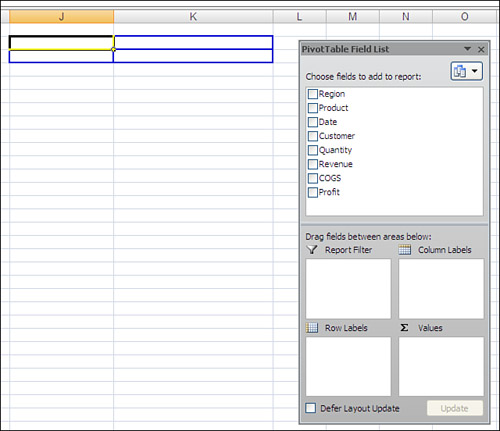
Click OK to create a blank pivot table. Instructions in the blank pivot table tell you to choose fields from the PivotTable Field List. The PivotTable Field List appears at the right side of your screen. A list of available fields is in the top of the task pane. Four drop zones, labeled Report Filter, Column Labels, Row Labels, and Σ Values appear at the bottom of the task pane (see Figure 13.3).
Click the Region and Revenue fields in the top section of the PivotTable Field List. Because the region field contains text data, it is automatically moved to the Row Labels drop zone. Because Revenue contains numeric data, it is automatically moved to the Σ Values drop zone.
Click the Product field in the top section of the PivotTable Field List and drag to the Column Labels drop zone in the bottom half of the PivotTable Field List. This adds a list of products stretching across the top row of your pivot table.


As shown in Figure 13.4, Excel has built a concise summary of your data in the pivot table.

After a pivot table has been created on your worksheet, you can easily change the data summarized in the report by dragging fields within the drop zones of the PivotTable Field List. In Figure 13.5, Customer was added to the Row Labels section of the existing pivot table.

By default, all new pivot tables are created in a new layout called Compact Form. In this layout, multiple Row fields appear in a single column at the left of the pivot table. Excel also puts the subtotals above the detail rows.
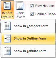
Although these changes might make for a better live pivot table, most of the pivot tables in this chapter will be converted to values to produce a static summary of the data. In these cases, you want to revert to the Outline layout that was the default in Excel 2003. The following steps in the user interface overcome these new default choices:
On the Design ribbon, choose Report Layout, Show in Outline Form, as shown in Figure 13.6.
On the Design ribbon, choose Subtotals, Show All Subtotals at the Bottom of Group.
On the Options ribbon, choose the Options icon on the left side of the ribbon. In the Layout & Format tab of the PivotTable Options dialog, type a zero next to For Empty Cells Show.
In this chapter, I do not mean to imply that you use VBA to build pivot tables to give to your clients. Rather, the purpose of this chapter is to remind you that pivot tables can be used as a means to an end; you can use a pivot table to extract a summary of data and then use that summary elsewhere.
Note
The code listings from this chapter are available for download at www.MrExcel.com/getcode2007.html.
Caution
Although the Excel user interface has new names for the various sections of a pivot table, VBA code continues to refer to the old names. Microsoft had to use this choice; otherwise, millions of lines of code would stop working in Excel 2007 when they referred to a page field rather than a filter field. Although the four sections of a pivot table in the Excel user interface are Report Filter, Column Labels, Row Labels, and Values, VBA continues to use the old terms of Page fields, Column fields, Row fields, and Data fields.
In Excel 2000 and later, you first build a pivot cache object to describe the input area of the data:
Dim WSD As Worksheet
Dim PTCache As PivotCache
Dim PT As PivotTable
Dim PRange As Range
Dim FinalRow As Long
Dim FinalCol As Long
Set WSD = Worksheets("PivotTable")

' Delete any prior pivot tables
For Each PT In WSD.PivotTables
    PT.TableRange2.Clear
Next PT

' Define input area and set up a Pivot Cache
FinalRow = WSD.Cells(Rows.Count, 1).End(xlUp).Row
FinalCol = WSD.Cells(1, Columns.Count).End(xlToLeft).Column
Set PRange = WSD.Cells(1, 1).Resize(FinalRow, FinalCol)
Set PTCache = ActiveWorkbook.PivotCaches.Add(SourceType:=xlDatabase, _
SourceData:=PRange)After defining the pivot cache, use the CreatePivotTable method to create a blank pivot table based on the defined pivot cache:
Set PT = PTCache.CreatePivotTable(TableDestination:=WSD.Cells(2, FinalCol + 2), _
    TableName:="PivotTable1")
In the CreatePivotTable method, you specify the output location and optionally give the table a name. After running this line of code, you have a strange-looking blank pivot table, like the one shown in Figure 13.7. You now have to use code to drop fields onto the table.
If you choose the Defer Layout Update setting in the user interface to build the pivot table, Excel does not recalculate the pivot table after you drop each field onto the table. By default in VBA, Excel calculates the pivot table as you execute each step of building the table. This could require the pivot table to be executed a half-dozen times before you get to the final result. To speed up your code execution, you can temporarily turn off calculation of the pivot table by using the ManualUpdate property:
PT.ManualUpdate = True
You can now run through the steps needed to lay out the pivot table. In the .AddFields method, you can specify one or more fields that should be in the row, column, or filter area of the pivot table.
The RowFields parameter enables you to define fields that appear in the Row Labels drop zone of the PivotTable Field List. The ColumnFields parameter corresponds to the Column Labels drop zone. The PageFields parameter corresponds to the Report Filter drop zone.
The following line of code populate a pivot table with two fields in the row area and one field in the column area:
' Set up the row & column fields
PT.AddFields RowFields:=Array("Region", "Customer"), _
    ColumnFields:="Product"
To add a field such as Revenue to the values area of the table, you change the Orientation property of the field to be xlDataField.
Excel is smart. When you build a report with revenue, it assumes you want to sum the revenue. But there is a problem. Suppose that one of the revenue cells is blank. When you build the pivot table, even though 99.9% of fields are numeric, Excel assumes you have alphanumeric data and offers to count this field. This is annoying. It seems to be an anomaly that, on one hand, you are expected to make sure that 100% of your cells have numeric data; on the other hand, however, the results of the pivot table are often filled with non-numeric blank cells.
When you build the pivot table in the Excel interface, you should take care in the Σ Values drop zone to notice that the field reads Count of Revenue rather than Sum of Revenue. At that point, the right course of action is to go back and fix the data, but what people usually do is double-click the Count of Revenue button and change it to Sum of Revenue.
In VBA, you should always explicitly define that you are creating a sum of revenue by explicitly setting the Function property to xlSum:
' Set up the data fields
With PT.PivotFields("Revenue")
    .Orientation = xlDataField
    .Function = xlSum
    .Position = 1
End With
At this point, you’ve given VBA all the settings required to correctly generate the pivot table. If you set ManualUpdate to False, Excel calculates and draws the pivot table. You can immediately thereafter set this back to True:
' Calc the pivot table
PT.ManualUpdate = False
PT.ManualUpdate = True
Your pivot table inherits the table style settings selected as the default on whatever computer happens to run the code. If you would like control over the final format, you can explicitly choose a table style. The following code applies banded rows and a medium table style:
' Format the pivot table
PT.ShowTableStyleRowStripes = True
PT.TableStyle2 = "PivotStyleMedium10"
At this point, you have a complete pivot table like the one shown in Figure 13.8.

Listing 13.1 shows the complete code used to generate the pivot table.
Example 13.1. Code to Generate a Pivot Table
Sub CreatePivot()
    Dim WSD As Worksheet
    Dim PTCache As PivotCache
    Dim PT As PivotTable
    Dim PRange As Range
    Dim FinalRow As Long
    Set WSD = Worksheets("PivotTable")

    ' Delete any prior pivot tables
    For Each PT In WSD.PivotTables
        PT.TableRange2.Clear
    Next PT

    ' Define input area and set up a Pivot Cache
    FinalRow = WSD.Cells(Application.Rows.Count, 1).End(xlUp).Row
    FinalCol = WSD.Cells(1, Application.Columns.Count). _
        End(xlToLeft).Column
    Set PRange = WSD.Cells(1, 1).Resize(FinalRow, FinalCol)
    Set PTCache = ActiveWorkbook.PivotCaches.Add(SourceType:= _
        xlDatabase, SourceData:=PRange.Address)

    ' Create the Pivot Table from the Pivot Cache
    Set PT = PTCache.CreatePivotTable(TableDestination:=WSD. _
        Cells(2, FinalCol + 2), TableName:="PivotTable1")

    ' Turn off updating while building the table
    PT.ManualUpdate = True

    ' Set up the row & column fields
    PT.AddFields RowFields:=Array("Region", "Customer"), _
        ColumnFields:="Product"

    ' Set up the data fields
    With PT.PivotFields("Revenue")
        .Orientation = xlDataField
        .Function = xlSum
        .Position = 1
    End With

    ' Calc the pivot table
    PT.ManualUpdate = False
    PT.ManualUpdate = True

    'Format the pivot table
    PT.ShowTableStyleRowStripes = True
    PT.TableStyle2 = "PivotStyleMedium10"

    WSD.Activate
    Range("J2").Select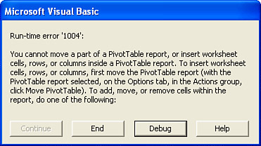
End SubAlthough pivot tables are incredible, they have annoying limitations. You cannot move or change just part of a pivot table. For example, try to run a macro that would delete Column Q, which contains the Grand Total column of the pivot table. The macro comes to a screeching halt with an error 1004, as shown in Figure 13.9. To get around this limitation, you can change the summary from a pivot table to just values.
Knowing the size of a pivot table in advance is difficult. If you run a report of transactional data on one day, you may or may not have sales from the West region, for example. This could cause your table to be either six or seven columns wide. Therefore, you should use the special property TableRange2 to refer to the entire resultant pivot table.
Because of the limitations of pivot tables, you should generally copy the results of a pivot table to a new location on the worksheet and then delete the original pivot table. The code in CreateSummaryReportUsingPivot() creates a small pivot table. Note that you can set the ColumnGrand and RowGrand properties of the table to False to prevent the totals from being added to the table.
PT.TableRange2 includes the entire pivot table. In Figure 13.10, TableRange2 includes the extra row at the top with the button Sum of Revenue. To eliminate that row, the code copies PT.TableRange2 but offsets this selection by one row by using .Offset(1, 0). Depending on the nature of your pivot table, you might need to use an offset of two or more rows to get rid of extraneous information at the top of the pivot table.
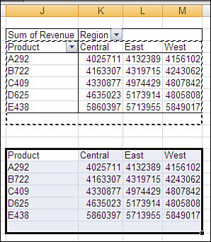
The code copies PT.TableRange2 and uses PasteSpecial on a cell five rows below the current pivot table. At that point in the code, your worksheet appears as shown in Figure 13.10. The table in J2 is a live pivot table, and the table in J12 is just the copied results.
You can then totally eliminate the pivot table by applying the Clear method to the entire table. If your code is then going on to do additional formatting, you should remove the pivot cache from memory by setting PTCache equal to Nothing.
The code in Listing 13.2 uses a pivot table to produce a summary from the underlying data. At the end of the code, the pivot table will be copied to static values and the pivot table will be cleared.
Example 13.2. Code to Produce a Static Summary from a Pivot Table
Sub CreateSummaryReportUsingPivot()
    ' Use a Pivot Table to create a static summary report
    ' with product going down the rows and regions across
    Dim WSD As Worksheet
    Dim PTCache As PivotCache
    Dim PT As PivotTable
    Dim PRange As Range
    Dim FinalRow As Long
    Set WSD = Worksheets("PivotTable")

    ' Delete any prior pivot tables
    For Each PT In WSD.PivotTables
        PT.TableRange2.Clear
    Next PT
    WSD.Range("J1:Z1").EntireColumn.Clear

    ' Define input area and set up a Pivot Cache
    FinalRow = WSD.Cells(Application.Rows.Count, 1).End(xlUp).Row
    FinalCol = WSD.Cells(1, Application.Columns.Count). _
        End(xlToLeft).Column
    Set PRange = WSD.Cells(1, 1).Resize(FinalRow, FinalCol)
    Set PTCache = ActiveWorkbook.PivotCaches.Add(SourceType:= _
        xlDatabase, SourceData:=PRange.Address)

    ' Create the Pivot Table from the Pivot Cache
    Set PT = PTCache.CreatePivotTable(TableDestination:=WSD. _
        Cells(2, FinalCol + 2), TableName:="PivotTable1")

    ' Turn off updating while building the table
    PT.ManualUpdate = True

    ' Set up the row fields
    PT.AddFields RowFields:="Product", ColumnFields:="Region"

    ' Set up the data fields
    With PT.PivotFields("Revenue")
        .Orientation = xlDataField
        .Function = xlSum
        .Position = 1
    End With

    With PT
        .ColumnGrand = False
        .RowGrand = False
        .NullString = "0"
    End With

    ' Calc the pivot table
    PT.ManualUpdate = False
    PT.ManualUpdate = True

    ' PT.TableRange2 contains the results. Move these to J12
    ' as just values and not a real pivot table.
    PT.TableRange2.Offset(1, 0).Copy
    WSD.Cells(5 + PT.TableRange2.Rows.Count, FinalCol + 2). _
        PasteSpecial xlPasteValues

    ' At this point, the worksheet looks like Figure 13.10
    ' Stop

    ' Delete the original Pivot Table & the Pivot Cache
    PT.TableRange2.Clear
    Set PTCache = Nothing

    WSD.Activate
    Range("J12").Select
End Sub
The code in Listing 13.2 creates the pivot table. It then copies the results as values and pastes them as values in J12:M13. Figure 13.10 (shown previously) shows an intermediate result just before the original pivot table is cleared.
So far, this chapter has walked you through building the simplest of pivot table reports. Pivot tables offer far more flexibility. The sections that follow present more complex reporting examples.
A typical report might provide a list of regions by product with revenue by year. This report could be given to product line managers to show them which customers are buying their products. In this example, you want to show the customers in descending order by revenue with years going across the columns. Figure 13.11 shows a sample report.

The key to producing this data quickly is to use a pivot table. Although pivot tables are incredible for summarizing data, you will often have to do some additional steps to achieve the desired result.
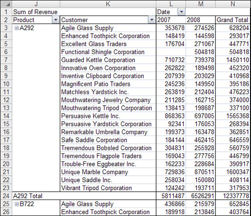
To create this report, start with a pivot table that has Product and Customer as Row fields, Date grouped by year as a Column field, and Sum of Revenue as the Data field. Figure 13.12 shows the default pivot table created with these settings.
Here are just a few of the annoyances that most pivot tables present in their default state:
The Outline view is horrible. In Figure 13.12, the value A292 appears in the Product column only once and is followed by 20 blank cells. This is the worst feature of pivot tables, and there is absolutely no way to correct it. Although humans can understand that this entire section is for A292 sales, it is radically confusing if your A292 section spills to a second or third page. Page 2 starts without any indication that the report is for A292 sales. If you intend to repurpose the data, you need the A292 sales value to be on every row.
The report contains blank cells rather than zeros. In Figure 13.12, the Functional Shingle had no sales in 2007. Excel produces a pivot table where cell L6 is blank rather than zero. This is simply bad form. Excel experts rely on being able to “ride the range,” using the End and arrow keys. Blank cells ruin this ability.
The title is boring. Most people would agree that Sum of Revenue is an annoying title.
Some captions are extraneous. Date floating in cell L1 of Figure 13.12 really does not belong in a report.
The default alphabetic sort order is rarely useful. Product line managers are going to want the top customers at the top of the list. It would be helpful to have the report sorted in descending order by revenue.
Depending on your computer’s default pivot table style, the borders could be ugly. Excel draws in a myriad of borders that really make the report look awful.
The default number format is General. It would be better to set this up as data with commas to serve as thousands separators, or perhaps even data in thousands or millions.
Pivot tables offer no obvious page-break logic. If you want to produce one report for each Line of Business manager, you would have to dig deep into the last setting of the back tab of the Field Settings dialog.
Because of the page-break problem, you might find it is easier to do away with the pivot table’s subtotal rows and have the
Subtotalmethod add subtotal rows with page breaks. You need a way to turn off the pivot table subtotal rows offered for Product in Figure 13.12. These rows show up automatically whenever you have two or more Row fields. If you had four Row fields, you would want to turn off the automatic subtotals for the three outermost Row fields.
Even with all these problems in default pivot tables, they are still the way to go. You can overcome each complaint, either by using special settings within the pivot table or by entering a few lines of code after the pivot table is created and then copied to a regular dataset.
People started complaining about the blank cells immediately when pivot tables were first introduced. Anyone using Excel 97 or later can easily replace blank cells with zeros. In the user interface, you can find the setting on the Layout & Format tab of the PivotTable Options dialog box. Choose the For Empty Cells, Show option and type 0 in the box.
The equivalent operation in VBA is to set the NullString property for the pivot table to "0".
In versions of Excel prior to 2007, multiple Row fields appeared in multiple columns. Three layouts are available in Excel 2007. The Compact layout squeezes all the Row fields into a single column.
To prevent this outcome and ensure that your pivot table is in the classic table layout, use this code:
PT.RowAxisLayout xlTabularRow
The Excel user interface offers an AutoSort option that enables you to show markets in descending order based on revenue. The equivalent code in VBA to sort the product field by descending revenue uses the AutoSort method:
PT.PivotFields("Customer").AutoSort Order:=xlDescending, _
Field:="Sum of Revenue"To change the number format in the user interface, choose a revenue field, and from the Options ribbon, choose Active Field, Field Settings, Number Format. Then choose an appropriate number format.
When you have large numbers, displaying the thousands separator helps the person reading the report. To set up this format in VBA code, use the following:
PT.PivotFields("Sum of Revenue").NumberFormat = "#,##0"Some companies have customers who typically buy thousands or millions of dollars’ worth of goods. You can display numbers in thousands by using a single comma after the number format. Of course, you need to include a K abbreviation to indicate that the numbers are in thousands:
PT.PivotFields("Sum of Revenue").NumberFormat = "#,##0,K"Local custom dictates the thousands abbreviation. If you are working for a relatively young computer company where everyone uses K for the thousands separator, you’re in luck because Microsoft makes it easy to use this abbreviation. However, if you work at a 100+ year-old soap company where you use M for thousands and MM for millions, you have a few more hurdles to jump. You are required to prefix the M character with a backslash to have it work:
PT.PivotFields("Sum of Revenue").NumberFormat = "#,##0,M"Alternatively, you can surround the M character with double quotation marks. To put double quotation marks inside a quoted string in VBA, you must put two sequential quotation marks. To set up a format in tenths of millions that uses the #,##0.0,,"MM" format, you would use this line of code:
PT.PivotFields("Sum of Revenue").NumberFormat = "#,##0.0,,""M"""In case it is difficult to read, the format for the code is quotation mark, pound, comma, pound, pound, zero, period, zero, comma, comma, quotation mark, quotation mark, M, quotation mark, quotation mark, quotation mark. The three quotation marks at the end are correct. You use two quotation marks to simulate typing one quotation mark in the custom number format box and a final quotation mark to close the string in VBA.
As soon as you have more than one Row field, Excel automatically adds subtotals for all but the innermost Row field. However, you might want to suppress subtotals for any number of reasons. Although accomplishing this task manually may be relatively simple, the VBA code to suppress subtotals is surprisingly complex.
You must set the Subtotals property equal to an array of 12 False values. Read the VBA help for all the gory details, but it goes something like this: The first False turns off automatic subtotals, the second False turns off the Sum subtotal, the third False turns off the Count subtotal, and so on. It is interesting that you have to turn off all 12 possible subtotals, even though Excel displays only one subtotal. This line of code suppresses the Product subtotal:
PT.PivotFields("Product").Subtotals = Array(False, False, False, False, _
    False, False, False, False, False, False, False, False)
A different technique is to turn on the first subtotal. This method automatically turns off the other 11 subtotals. You can then turn off the first subtotal to make sure that all subtotals are suppressed:
PT.PivotFields("Product").Subtotals(1) = True
PT.PivotFields("Product").Subtotals(1) = FalseBecause you are going to be using VBA code to add automatic subtotals, you can get rid of the Grand Total row. If you turn off Grand Total for Rows, you delete the column called Grand Total. Therefore, to get rid of the Grand Total row, you must uncheck Grand Total for Columns. This is handled in the code with the following line:
PT.ColumnGrand = False
You’ve reached the end of the adjustments that you can make to the pivot table. To achieve the final report, you have to make the remaining adjustments after converting the pivot table to regular data.
Figure 13.13 shows the pivot table with all the adjustments described in the preceding sections and with PT.TableRange2 selected.

Say you want to build the report in a new workbook so that it can be easily mailed to the product managers. Doing this is fairly easy. To make the code more portable, assign object variables to the original workbook, new workbook, and first worksheet in the new workbook. At the top of the procedure, add these statements:
Dim WSR As Worksheet
Dim WBO As Workbook
Dim WBN As Workbook
Set WBO = ActiveWorkbook
Set WSD = Worksheets("Pivot Table")
After the pivot table has been successfully created, build a blank Report workbook with this code:
' Create a New Blank Workbook with one Worksheet
Set WBN = Workbooks.Add(xlWorksheet)
Set WSR = WBN.Worksheets(1)
WSR.Name = "Report"
' Set up Title for Report
With WSR.Range("A1")
    .Value = "Revenue by Customer and Year"
    .Font.Size = 14
End WithImagine that you have submitted the pivot table in Figure 13.13, and your manager hates the borders, hates the title, and hates the word Date in cell L2. You can solve all three of these problems by excluding the first row(s) of PT.TableRange2 from the .Copy method and then using PasteSpecial(xlPasteValuesAndNumberFormats) to copy the data to the report sheet.
Tip
In Excel 2000 and earlier, xlPasteValuesAndNumberFormats was not available. You had to use Paste Special twice: once as xlPasteValues and once as xlPasteFormats.
In the current example, the .TableRange2 property includes only one row to eliminate, Row 2, as shown in Figure 13.13. If you had a more complex pivot table with several Column fields or one or more page fields, you would have to eliminate more than just the first row of the report. It helps to run your macro to this point, look at the result, and figure out how many rows you need to delete. You can effectively not copy these rows to the report by using the Offset property. Copy the TableRange2 property, offset by one row. Purists will note that this code copies one extra blank row from below the pivot table, but this really does not matter because the row is blank. After copying, you can erase the original pivot table and destroy the pivot cache:
' Copy the Pivot Table data to row 3 of the Report sheet
' Use Offset to eliminate the title row of the pivot table
PT.TableRange2.Offset(1, 0).Copy
WSR. Range("A3").PasteSpecial Paste:=xlPasteValuesAndNumberFormats
PT.TableRange2.Clear
Set PTCache = Nothing
Note that you use the Paste Special option to paste just values and number formats. This gets rid of both borders and the pivot nature of the table. You might be tempted to use the No Borders option under Paste, but this keeps the data in a pivot table, and you won’t be able to insert new rows in the middle of the data.
The report is almost complete. You are nearly a Data, Subtotals command away from having everything you need. Before you can use the Subtotals command, however, you need to fill in all the blank cells in the Outline view of Column A.
Fixing the Outline view requires just a few obscure steps. Here are the steps in the user interface:
Select all the cells in Column A that make up the report.
From the Home ribbon, select Editing, Find & Select, Go to Special to bring up the Go to Special dialog box. Select Blanks to select only the blank cells.
Enter an R1C1 style formula to fill the blank with the cell above it. This formula is
=R[-1]C. In the user interface, you would type an equal sign, press the up-arrow key, and then press Ctrl+Enter.Reselect all the cells in Column A that make up the report. This step is necessary because the Paste Special step cannot work with noncontiguous selections.
Copy the formulas in Column A and convert them to values by choosing Clipboard, Paste, Paste Values from the Home ribbon.
Fixing the Outline view in VBA requires fewer steps. The equivalent VBA logic is shown here:
Find the last row of the report.
Enter the formula
=R[-1]Cin the blank cells in A.Change those formulas to values. The code to do this follows:
Dim FinalReportRow as Long
    ' Fill in the Outline view in column A
    ' Look for last row in column B since many rows
    ' in column A are blank
FinalReportRow = WSR.Cells(Rows.Count, 2).End(xlUp).Row
With Range("A3").Resize(FinalReportRow - 2, 1)
    With .SpecialCells(xlCellTypeBlanks)
        .FormulaR1C1 = "=R[-1]C"
    End With
    .Value = .Value
End With
The last steps for the report involve some basic formatting tasks and then adding the subtotals. You can bold and right-justify the headings in Row 3. Set up Rows 1 through 3 so that the top three rows print on each page:
' Do some basic formatting
' Autofit columns, bold the headings, right-align
Selection.Columns.AutoFit
Range("A3").EntireRow.Font.Bold = True
Range("A3").EntireRow.HorizontalAlignment = xlRight
Range("A3:B3").HorizontalAlignment = xlLeft

' Repeat rows 1-3 at the top of each page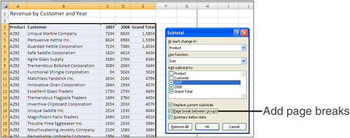
WSR.PageSetup.PrintTitleRows = "$1:$3"Automatic subtotals are a powerful feature found on the Data ribbon. Figure 13.14 shows the Subtotal dialog box. Note the option Page Break Between Groups.
If you were sure that you would always have two years and a total, the code to add subtotals for each Line of Business group would be the following:
' Add Subtotals by Product.
' Be sure to add a page break at each change in product
Selection.Subtotal GroupBy:=1, Function:=xlSum, TotalList:=Array(3, 4, 5), _
    PageBreaks:=True
However, this code fails if you have more or less than three years. The solution is to use the following convoluted code to dynamically build a list of the columns to total, based on the number of columns in the report:
Dim TotColumns()
Dim I as Integer
FinalCol = Cells(3, Columns.Count).End(xlToLeft).Column
ReDim Preserve TotColumns(1 To FinalCol - 2)
For i = 3 To FinalCol
    TotColumns(i - 2) = i
Next i
Selection.Subtotal GroupBy:=1, Function:=xlSum, TotalList:=TotColumns,_
     Replace:=True, PageBreaks:=True, SummaryBelowData:=True
Finally, with the new totals added to the report, you need to autofit the numeric columns again with this code:
Dim GrandRow as Long
' Make sure the columns are wide enough for totals
GrandRow = Cells(Rows.Count, 1).End(xlUp).Row
Cells(3, 3).Resize(GrandRow - 2, FinalCol - 2).Columns.AutoFit
Cells(GrandRow, 3).Resize(1, FinalCol - 2).NumberFormat = "#,##0,K"
' Add a page break before the Grand Total row, otherwise
' the product manager for the final Line will have two totals
WSR.HPageBreaks.Add Before:=Cells(GrandRow, 1)
Listing 13.3 produces the product line manager reports in a few seconds.
Example 13.3. Code That Produces the Product Line Report in Figure 13.15
Sub ProductLineReport()
' Product and Customer as Row
' Years as Column
Dim WSD As Worksheet
Dim PTCache As PivotCache
Dim PT As PivotTable
Dim PRange As Range
Dim FinalRow As Long
Dim TotColumns()
Set WSD = Worksheets("PivotTable")
Dim WSR As Worksheet
Dim WBO As Workbook
Dim WBN As Workbook
Set WBO = ActiveWorkbook
' Delete any prior pivot tables
For Each PT In WSD.PivotTables
PT.TableRange2.Clear
Next PT
WSD.Range("J1:Z1").EntireColumn.Clear
' Define input area and set up a Pivot Cache
FinalRow = WSD.Cells(Application.Rows.Count, 1).End(xlUp).Row
FinalCol = WSD.Cells(1, Application.Columns.Count). _
End(xlToLeft).Column
Set PRange = WSD.Cells(1, 1).Resize(FinalRow, FinalCol)
Set PTCache = ActiveWorkbook.PivotCaches.Add(SourceType:= _
xlDatabase, SourceData:=PRange.Address)
' Create the Pivot Table from the Pivot Cache
Set PT = PTCache.CreatePivotTable(TableDestination:=WSD. _
Cells(2, FinalCol + 2), TableName:="PivotTable1")
' Turn off updating while building the table
PT.ManualUpdate = True
' Set up the row fields
PT.AddFields RowFields:=Array("Product", _
"Customer"), ColumnFields:="Date"
' Set up the data fields
With PT.PivotFields("Revenue")
.Orientation = xlDataField
.Function = xlSum
.Position = 1
End With
' Make sure to get tabular layout
' instead of the new compact layout
PT.RowAxisLayout xlTabularRow
' Calc the pivot table
PT.ManualUpdate = False
PT.ManualUpdate = True
' Group by Year
WSD.Activate
Cells(3, FinalCol + 4).Group Start:=True, End:=True, _
Periods:=Array(False, False, False, False, False, False, True)
' Move Date to columns
PT.PivotFields("Date").Orientation = xlColumnField
PT.PivotFields("Customer").Orientation = xlRowField
' Format the Revenue fields
PT.PivotFields("Sum of Revenue").NumberFormat = "#,##0,K"
' Turn off the subtotals by product
PT.PivotFields("Product").Subtotals(1) = True
PT.PivotFields("Product").Subtotals(1) = False
PT.ColumnGrand = False
' Ensure that we get zeroes instead of blanks in the data area
PT.NullString = "0"
' Sort customers descending by sum of revenue
PT.PivotFields("Customer").AutoSort Order:=xlDescending, _
Field:="Sum of Revenue"
' Calc the pivot table
PT.ManualUpdate = False
PT.ManualUpdate = True
' At this point, the data is like Figure 13.13
PT.TableRange2.Select
' Stop
' Create a New Blank Workbook with one Worksheet
Set WBN = Workbooks.Add(xlWBATWorksheet)
Set WSR = WBN.Worksheets(1)
WSR.Name = "Report"
' Set up Title for Report
With WSR.[A1]
.Value = "Revenue by Customer and Year"
.Font.Size = 14
End With
' Copy the Pivot Table data to row 3 of the Report sheet
' Use Offset to eliminate the title row of the pivot table
PT.TableRange2.Offset(1, 0).Copy
WSR.[A3].PasteSpecial Paste:=xlPasteValuesAndNumberFormats
PT.TableRange2.Clear
Set PTCache = Nothing
' Fill in the Outline view in column A
' Look for last row in column B since many rows
' in column A are blank
FinalReportRow = WSR.Range("B65536").End(xlUp).Row
With Range("A3").Resize(FinalReportRow - 2, 1)
With .SpecialCells(xlCellTypeBlanks)
.FormulaR1C1 = "=R[-1]C"
End With
.Value = .Value
End With
' Do some basic formatting
' Autofit columns, bold the headings, right-align
Selection.Columns.AutoFit
Range("A3").EntireRow.Font.Bold = True
Range("A3").EntireRow.HorizontalAlignment = xlRight
Range("A3:B3").HorizontalAlignment = xlLeft
' Repeat rows 1-3 at the top of each page
WSR.PageSetup.PrintTitleRows = "$1:$3"
' Add subtotals
FinalCol = Cells(3, 255).End(xlToLeft).Column
ReDim Preserve TotColumns(1 To FinalCol - 2)
For i = 3 To FinalCol
TotColumns(i - 2) = i
Next i
Selection.Subtotal GroupBy:=1, Function:=xlSum, _
TotalList:=TotColumns, Replace:=True, _
PageBreaks:=True, SummaryBelowData:=True
' Make sure the columns are wide enough for totals
GrandRow = Cells(Rows.Count, 1).End(xlUp).Row
Cells(3, 3).Resize(GrandRow - 2, FinalCol - 2).Columns.AutoFit
Cells(GrandRow, 3).Resize(1, FinalCol - 2).NumberFormat = "#,##0,K"
' Add a page break before the Grand Total row, otherwise
' the product manager for the final Line will have two totals
WSR.HPageBreaks.Add Before:=Cells(GrandRow, 1)
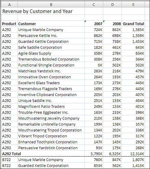
End SubFigure 13.15 shows the report produced by this code.
So far, you have built some powerful summary reports, but you’ve touched only a portion of the powerful features available in pivot tables. The preceding example produced a report but had only one Data field. It is possible to have multiple fields in the Σ Values section of a pivot report. The data in this example includes not just revenue, but also a count of customers.
When you have two or more Data fields, you have a choice of placing the Data fields in one of four locations. By default, Excel builds the pivot report with the Data field as the innermost Column field. It is often preferable to have the Data field as the outermost Row field.
When a pivot table is going to have more than one Data field, you have a virtual field named Σ Values in the drop zones of the PivotTable Field List. In VBA, this equivalent virtual field is named Data.
To arrange the fields so that the data field is the innermost row, as shown in Figure 13.16, you would use this AddFields line:
PT.AddFields RowFields:=Array("Product", "Data")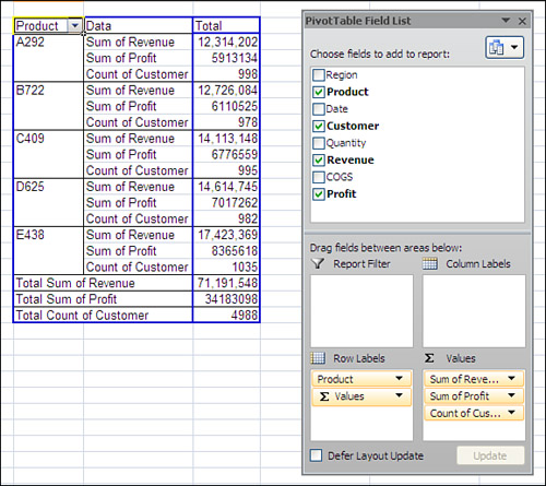
If you move the Data field as the first Row field, you will have the view shown in Figure 13.17. In this version, Total Sum of Revenue appears 10 rows away from all the other revenue fields. The view shown in Figure 13.17 would use this code:
PT.AddFields RowFields:=Array("Data", "Product")
One view that would make sense would have Data as the only Column field:
PT.AddFields RowFields:="Product", ColumnFields:="Data"
After adding a Column field called Data, you would then go on to define three Data fields:
' Set up the data fields
With PT.PivotFields("Revenue")
    .Orientation = xlDataField
    .Function = xlSum
    .Position = 1
    .NumberFormat = "#,##0,K"
End With

With PT.PivotFields("Profit")
    .Orientation = xlDataField
    .Function = xlSum
    .Position = 2
    .NumberFormat = "#,##0"
End With

With PT.PivotFields("Customer")
    .Orientation = xlDataField
    .Function = xlCount
    .Position = 3
    .NumberFormat = "#,##0"
End With
Figure 13.18 shows the report produced by the previous code.

Pivot tables offer two types of formulas. The most useful type defines a formula for a calculated field. This adds a new field to the pivot table. Calculations for calculated fields are always done at the summary level. If you define a calculated field for average price as Revenue divided by Units Sold, Excel first adds the total revenue and total quantity, and then it does the division of these totals to get the result. In many cases, this is exactly what you need. If your calculation does not follow the associative law of mathematics, it might not work as you expect.
To set up a Calculated field, use the Add method with the CalculatedFields object. You have to specify a field name and a formula. Note that if you create a field called Profit Percent, the default pivot table produces a field called Sum of Profit Percent. This title is misleading and downright silly. The solution is to use the Name property when defining the Data field to replace Sum of Profit Percent with something such as GP Pct. Note that this name must differ from the name for the Calculated field.
Listing 13.4 produces the report shown in Figure 13.19.

Example 13.4. Code That Calculates a Profit Percent as a Second Data Field
Sub CalculatedField()
    'Listing 13.4
    Dim WSD As Worksheet
    Dim PTCache As PivotCache
    Dim PT As PivotTable
    Dim PRange As Range
    Dim FinalRow As Long

    Set WSD = Worksheets("PivotTable")
    Dim WSR As Worksheet
    Dim WBO As Workbook
    Dim WBN As Workbook
    Set WBO = ActiveWorkbook

    ' Delete any prior pivot tables
    For Each PT In WSD.PivotTables
        PT.TableRange2.Clear
    Next PT
    WSD.Range("J1:Z1").EntireColumn.Clear

    ' Define input area and set up a Pivot Cache
    FinalRow = WSD.Cells(Application.Rows.Count, 1).End(xlUp).Row
    FinalCol = WSD.Cells(1, Application.Columns.Count). _
        End(xlToLeft).Column
    Set PRange = WSD.Cells(1, 1).Resize(FinalRow, FinalCol)
    Set PTCache = ActiveWorkbook.PivotCaches.Add(SourceType:= _
        xlDatabase, SourceData:=PRange.Address)

    ' Create the Pivot Table from the Pivot Cache
    Set PT = PTCache.CreatePivotTable(TableDestination:=WSD. _
        Cells(2, FinalCol + 2), TableName:="PivotTable1")

    ' Turn off updating while building the table
    PT.ManualUpdate = True

    ' Set up the row fields
    PT.AddFields RowFields:="Product", ColumnFields:="Data"

    ' Define Calculated Fields
    PT.CalculatedFields.Add Name:="ProfitPercent", Formula:="=Profit/Revenue"

    ' Set up the data fields
    With PT.PivotFields("Revenue")
        .Orientation = xlDataField
        .Function = xlSum
        .Position = 1
        .NumberFormat = "#,##0"
    End With

    With PT.PivotFields("Profit")
        .Orientation = xlDataField
        .Function = xlSum
        .Position = 2
        .NumberFormat = "#,##0"
    End With

    With PT.PivotFields("ProfitPercent")
        .Orientation = xlDataField
        .Function = xlSum
        .Position = 3
        .NumberFormat = "#0.0%"
        .Name = "GP Pct"
    End With

    ' Ensure that we get zeros instead of blanks in the data area
    PT.NullString = "0"

    ' Calc the pivot table
    PT.ManualUpdate = False
    PT.ManualUpdate = True

    WSD.Activate
    Range("J2").Select

End Sub
Calculated Items
Suppose that in your company one manager is responsible for the product lines A292 and C409. The idea behind a calculated item is that you can define a new item along the Product field to calculate the total of these two items. Listing 13.5 produces the report shown in Figure 13.20.

Example 13.5. Code That Adds a New Item along the Product Dimension
Sub CalcItemsProblem()
    ' Listing 13.5
    Dim WSD As Worksheet
    Dim PTCache As PivotCache
    Dim PT As PivotTable
    Dim PRange As Range
    Dim FinalRow As Long

    Set WSD = Worksheets("PivotTable")
    Dim WSR As Worksheet

    ' Delete any prior pivot tables
    For Each PT In WSD.PivotTables
        PT.TableRange2.Clear
    Next PT
    WSD.Range("J1:Z1").EntireColumn.Clear

    ' Define input area and set up a Pivot Cache
    FinalRow = WSD.Cells(Application.Rows.Count, 1).End(xlUp).Row
    FinalCol = WSD.Cells(1, Application.Columns.Count). _
        End(xlToLeft).Column
    Set PRange = WSD.Cells(1, 1).Resize(FinalRow, FinalCol)
    Set PTCache = ActiveWorkbook.PivotCaches.Add(SourceType:= _
        xlDatabase, SourceData:=PRange.Address)

    ' Create the Pivot Table from the Pivot Cache
    Set PT = PTCache.CreatePivotTable(TableDestination:=WSD. _
        Cells(2, FinalCol + 2), TableName:="PivotTable1")

    ' Turn off updating while building the table
    PT.ManualUpdate = True

    ' Set up the row fields
    PT.AddFields RowFields:="Product"

    ' Define calculated item along the product dimension
    PT.PivotFields("Product").CalculatedItems _
        .Add "MyDivision", "='A292'+'C409'"
    ' Resequence so that the report has A292 and C409 first
    PT.PivotFields("Product"). _
        PivotItems("A292").Position = 1
    PT.PivotFields("Product"). _
        PivotItems("C409").Position = 2
    PT.PivotFields("Product"). _
        PivotItems("MyDivision").Position = 3

    ' Set up the data fields
    With PT.PivotFields("Revenue")
        .Orientation = xlDataField
        .Function = xlSum
        .Position = 1
        .NumberFormat = "#,##0"
    End With

    ' Ensure that we get zeros instead of blanks in the data area
    PT.NullString = "0"

    ' Calc the pivot table
    PT.ManualUpdate = False
    PT.ManualUpdate = True
    WSD.Activate
    Range("J2").Select

End Sub
Look closely at the results shown in Figure 13.20. The calculation for MyDivision is correct. The approximate $26 million for the MyDivision is the sum of $12 million for A292 and $14 million of C409. However, the grand total should be about $71 million. Instead, Excel gives you a grand total of $97 million. The total revenue for the company just increased by $26 million. Excel gives the wrong grand total when a field contains both regular and calculated items. The only plausible method for dealing with this situation is to attempt to hide the products that make up MyDivision:
With PT.PivotFields("Product")
    .PivotItems("A292").Visible = False
    .PivotItems("C409").Visible = False
End With
Figure 13.21 shows the results.

With transactional data, you often find your date-based summaries having one row per day. Although daily data might be useful to a plant manager, many people in the company want to see totals by month, or by quarter, and year.
The great news is that Excel handles the summarization of dates in a pivot table with ease. For anyone who has ever had to use the arcane formula =A2-DAY(A2)+1 to change daily dates into monthly dates, you will appreciate the ease with which you can group transactional data into months or quarters.
In Figure 13.22, select one cell that contains a date. From the Options ribbon, choose Group Field. In the Grouping dialog, choose to group by Months, Quarters, and Years.

Caution
Never choose to group by only months without including years. If you do this, Excel combines January from this year and January from last year into a single item called January. Although this is great for seasonality analyses, it is rarely what you want in a summary. Always choose Years and Months in the Grouping dialog.
Creating a group with VBA is a bit quirky. The .Group method can be applied to only a single cell in the pivot table, and that cell must contain a date or the Date field label. This is the first example in this chapter where you must allow VBA to calculate an intermediate pivot table result.
You must define a pivot table with Invoice Date in the Row field. Turn off ManualCalculation to allow the Date field to be drawn. You can then use the LabelRange property to locate the date label and apply the .Group method.
PT.PivotFields("Date").LabelRange.GroupTo specify how to group the Date field, you have to pass an array of seven True/False values. The first value corresponds to the Seconds selection in the Grouping dialog. The next value corresponds to Minutes, then Hours, Days, Months, Quarters, and Years. In this example, you want to group by months, quarters, and years, so the Periods argument is as follows:
Periods:=Array(False, False, False, False, True, True, True)
Figure 13.23 shows the result of Listing 13.6.

Example 13.6. Code That Uses the Group Feature to Roll Daily Dates Up to Monthly Dates
Sub ReportByMonth()
    ' Listing 13.6
    Dim WSD As Worksheet
    Dim PTCache As PivotCache
    Dim PT As PivotTable
    Dim PRange As Range
    Dim FinalRow As Long

    Set WSD = Worksheets("PivotTable")
    Dim WSR As Worksheet

    ' Delete any prior pivot tables
    For Each PT In WSD.PivotTables
        PT.TableRange2.Clear
    Next PT
    WSD.Range("R1:AZ1").EntireColumn.Clear

    ' Define input area and set up a Pivot Cache
    FinalRow = WSD.Cells(Rows.Count, 1).End(xlUp).Row
    FinalCol = WSD.Cells(1, Columns.Count). _
        End(xlToLeft).Column
    Set PRange = WSD.Cells(1, 1).Resize(FinalRow, FinalCol)
    Set PTCache = ActiveWorkbook.PivotCaches.Add(SourceType:= _
        xlDatabase, SourceData:=PRange.Address)

    ' Create the Pivot Table from the Pivot Cache
    Set PT = PTCache.CreatePivotTable(TableDestination:=WSD. _
        Cells(2, FinalCol + 2), TableName:="PivotTable1")

    ' Turn off updating while building the table
    PT.ManualUpdate = True

    ' Set up the row fields
    PT.AddFields RowFields:="Date", ColumnFields:="Region"

    ' Set up the data fields
    With PT.PivotFields("Revenue")
        .Orientation = xlDataField
        .Function = xlSum
        .Position = 1
        .NumberFormat = "#,##0"
    End With

    ' Ensure that we get zeros instead of blanks in the data area
    PT.NullString = "0"

    ' Calc the pivot table to allow the date label to be drawn
    PT.ManualUpdate = False
    PT.ManualUpdate = True
    WSD.Activate

    ' Group ShipDate by Month, Quarter, Year
    PT.PivotFields("Date").LabelRange.Group _
        Start:=True, End:=True, _
        Periods:=Array(False, False, False, False, True, True, True)

    ' Calc the pivot table
    PT.ManualUpdate = False
    PT.ManualUpdate = True
    WSD.Activate
    Range("R1").Select

End SubYou probably noticed that Excel enables you to group by day, month, quarter, and year. There is no standard grouping for week. You can, however, define a group that bunches groups of seven days.
By default, Excel starts the week based on the first date found in the data. This means that the default week would run from Tuesday, January 2, 2007, through Monday, January 8, 2007. You can override this by changing the Start parameter from True to an actual date.
Figuring out the correct first date requires some basic Excel functions. You can use the MIN function to find the earliest date in your pivot table with this code:
FirstDate = Application.WorksheetFunction.Min( _
    PT.PivotFields("Date").DataRange)
You can then use the WeekDay function to determine how many days to adjust the start date:
WhichDay = Application.WorksheetFunction.Weekday(FirstDate, 3)
StartDate = FirstDate - WhichDay
After you have determined the date that the first week should start on, use the following code to group the field by groups of seven days:
PT.PivotFields("Date").LabelRange.Group _
    Start:=StartDate, End:=True, By:=7, _
    Periods:=Array(False, False, False, True, False, False, False)
Caution
There is one limitation to grouping by week. When you group by week, you cannot also group by any other measure. For example, grouping by week and quarter is not valid.
Listing 13.7 creates the report shown in Figure 13.24.

Example 13.7. Code That Uses the Group Feature to Roll Daily Dates Up to Weekly Dates
Sub ReportByWeek()
    ' Listing 13.7
    Dim WSD As Worksheet
    Dim PTCache As PivotCache
    Dim PT As PivotTable
    Dim PRange As Range
    Dim FinalRow As Long

    Set WSD = Worksheets("PivotTable")
    Dim WSR As Worksheet

    ' Delete any prior pivot tables
    For Each PT In WSD.PivotTables
        PT.TableRange2.Clear
    Next PT
    WSD.Range("J1:Z1").EntireColumn.Clear

    ' Define input area and set up a Pivot Cache
    FinalRow = WSD.Cells(Application.Rows.Count, 1).End(xlUp).Row
    FinalCol = WSD.Cells(1, Application.Columns.Count). _
        End(xlToLeft).Column
    Set PRange = WSD.Cells(1, 1).Resize(FinalRow, FinalCol)
    Set PTCache = ActiveWorkbook.PivotCaches.Add(SourceType:= _
        xlDatabase, SourceData:=PRange.Address)

    ' Create the Pivot Table from the Pivot Cache
    Set PT = PTCache.CreatePivotTable(TableDestination:=WSD. _
        Cells(2, FinalCol + 2), TableName:="PivotTable1")

    ' Turn off updating while building the table
    PT.ManualUpdate = True

    ' Set up the row fields
    PT.AddFields RowFields:="Date", ColumnFields:="Region"

    ' Set up the data fields
    With PT.PivotFields("Revenue")
        .Orientation = xlDataField
        .Function = xlSum
        .Position = 1
        .NumberFormat = "#,##0"
    End With

    ' Ensure that we get zeros instead of blanks in the data area
    PT.NullString = "0"

    ' Calc the pivot table to allow the date label to be drawn
    PT.ManualUpdate = False
    PT.ManualUpdate = True
    WSD.Activate

    ' Group Date by Week.
    'Figure out the first Monday before the minimum date
    FirstDate = Application.WorksheetFunction.Min( _
        PT.PivotFields("Date").DataRange)
    WhichDay = Application.WorksheetFunction.Weekday(FirstDate, 3)
    StartDate = FirstDate - WhichDay
    PT.PivotFields("Date").LabelRange.Group _
        Start:=StartDate, End:=True, By:=7, _
        Periods:=Array(False, False, False, True, False, False, False)

    ' Calc the pivot table
    PT.ManualUpdate = False
    PT.ManualUpdate = True
    WSD.Activate
    Range("J2").Select

End SubRecall in the last section how Excel adds field names when you group by month and year. The less-aggregated measure (month) inherits the name of the original field. Any more-aggregated measures receive the name of the grouping—for example, Years.
Your manufacturing plant might be concerned with a measure of how far in advance the orders are received. If the plant has a 12-week lead time to procure components, they would love to have all orders placed 13 weeks in advance. When this doesn’t happen, it is critical that you have an excellent forecasting system in place to accurately predict orders.
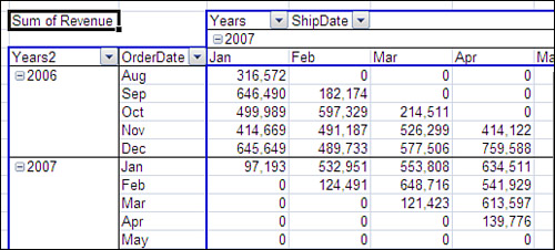
If you can add an OrderDate field to your transactional data, you could build a table to show how much revenue is received x months in advance of the ship date.
Follow these steps to set up an interesting potential anomaly:
Build a pivot table with
ShipDatein the Column area,OrderDatein the Row area, andRevenuein the Data area.Allow the pivot table to calculate.
Group ShipDate by month and year. This creates fields called ShipDate and Year.
Allow the pivot table to calculate. If you attempt to group the order Date field before calculating the results of step 3, you will get an error.
Group OrderDate by month and year. This creates a field called OrderDate with data by month. The grouping of OrderDate by year would tend to also be called Year, but Excel instead calls it Year2. Unless you know that the code grouped ShipDate before OrderDate, you would never know that Year2 referred to the order date and not the ship date.
Versions of Excel since 2000 correctly deal with the second set of grouped Date fields by changing the field name to Year2 rather than having a second Year.
Listing 13.8 creates the report shown in Figure 13.25.
Example 13.8. Code Used to Create the Order Lead Time Report
Sub MeasureLeadtime2007()
    ' Listing 13.8
    Dim WSD As Worksheet
    Dim PTCache As PivotCache
    Dim PT As PivotTable
    Dim PRange As Range
    Dim FinalRow As Long

    Set WSD = Worksheets("LeadTime")
    Dim WSR As Worksheet

    ' Delete any prior pivot tables
    For Each PT In WSD.PivotTables
        PT.TableRange2.Clear
    Next PT

    ' Define input area and set up a Pivot Cache
    FinalRow = WSD.Cells(Application.Rows.Count, 1).End(xlUp).Row
    FinalCol = WSD.Cells(1, Application.Columns.Count). _
        End(xlToLeft).Column
    Set PRange = WSD.Cells(1, 1).Resize(FinalRow, FinalCol)
    Set PTCache = ActiveWorkbook.PivotCaches.Add(SourceType:= _
        xlDatabase, SourceData:=PRange.Address)

    ' Create the Pivot Table from the Pivot Cache
    Set PT = PTCache.CreatePivotTable(TableDestination:=WSD. _
        Cells(2, FinalCol + 2), TableName:="PivotTable1")

    ' Turn off updating while building the table
    PT.ManualUpdate = True

    ' Set up the row fields
    PT.AddFields RowFields:="OrderDate", ColumnFields:="ShipDate"

    ' Set up the data fields
    With PT.PivotFields("Revenue")
        .Orientation = xlDataField
        .Function = xlSum
        .Position = 1
        .NumberFormat = "#,##0"
    End With

    ' Ensure that we get zeros instead of blanks in the data area
    PT.NullString = "0"

    ' Calc the pivot table to allow the date label to be drawn
    PT.ManualUpdate = False
    PT.ManualUpdate = True
    WSD.Activate

    ' Group ShipDate by Month and Year
    PT.PivotFields("ShipDate").LabelRange.Group Start:=True, End:=True, _
        Periods:=Array(False, False, False, False, True, False, True)

    ' Calc the pivot table to allow the date label to be drawn
    PT.ManualUpdate = False
    PT.ManualUpdate = True

    ' Group OrderDate by Month and Year
    PT.PivotFields("OrderDate").LabelRange.Group Start:=True, End:=True, _
        Periods:=Array(False, False, False, False, True, False, True)

    ' Calc the pivot table
    PT.ManualUpdate = False
    PT.ManualUpdate = True
    WSD.Activate
    Range("K2").Select
End Sub
You may be a pivot table pro and never have run into some of the really advanced techniques available with pivot tables. The following sections discuss such techniques.
If you are designing an executive dashboard utility, you might want to spotlight the top five customers.
As with the AutoSort option, you could be a pivot table pro and never have stumbled across the AutoShow feature in Excel. This setting lets you select either the top or bottom n records based on any Data field in the report.
The code to use AutoShow in VBA uses the .AutoShow method:
' Show only the top 5 Customers
PT.PivotFields("Customer").AutoShow Top:=xlAutomatic, Range:=xlTop, _
    Count:=5, Field:= "Sum of Revenue"
When you create a report using the .AutoShow method, it is often helpful to copy the data and then go back to the original pivot report to get the totals for all markets. In the code shown in Listing 13.9, this is achieved by removing the Customer field from the pivot table and copying the grand total to the report. Listing 13.9 produces the report shown in Figure 13.26.
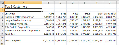
Example 13.9. Code Used to Create the Top 5 Customers Report
Sub Top5Customers()
    ' Listing 13.9
    ' Produce a report of the top 5 customers
    Dim WSD As Worksheet
    Dim WSR As Worksheet
    Dim WBN As Workbook
    Dim PTCache As PivotCache
    Dim PT As PivotTable
    Dim PRange As Range
    Dim FinalRow As Long
    Set WSD = Worksheets("PivotTable")

    ' Delete any prior pivot tables
    For Each PT In WSD.PivotTables
        PT.TableRange2.Clear
    Next PT
    WSD.Range("J1:Z1").EntireColumn.Clear

    ' Define input area and set up a Pivot Cache
    FinalRow = WSD.Cells(Application.Rows.Count, 1).End(xlUp).Row
    FinalCol = WSD.Cells(1, Application.Columns.Count). _
        End(xlToLeft).Column
    Set PRange = WSD.Cells(1, 1).Resize(FinalRow, FinalCol)
    Set PTCache = ActiveWorkbook.PivotCaches.Add(SourceType:= _
        xlDatabase, SourceData:=PRange.Address)

    ' Create the Pivot Table from the Pivot Cache
    Set PT = PTCache.CreatePivotTable(TableDestination:=WSD. _
        Cells(2, FinalCol + 2), TableName:="PivotTable1")

    ' Turn off updating while building the table
    PT.ManualUpdate = True

    ' Set up the row fields
    PT.AddFields RowFields:="Customer", ColumnFields:="Product"

    ' Set up the data fields
    With PT.PivotFields("Revenue")
        .Orientation = xlDataField
        .Function = xlSum
        .Position = 1
        .NumberFormat = "#,##0"
        .Name = "Total Revenue"
    End With

    ' Ensure that we get zeros instead of blanks in the data area
    PT.NullString = "0"

    ' Sort customers descending by sum of revenue
    PT.PivotFields("Customer").AutoSort Order:=xlDescending, _
        Field:="Total Revenue"

    ' Show only the top 5 customers
    PT.PivotFields("Customer").AutoShow Type:=xlAutomatic, Range:=xlTop, _
        Count:=5, Field:="Total Revenue"

    ' Calc the pivot table to allow the date label to be drawn
    PT.ManualUpdate = False
    PT.ManualUpdate = True

    ' Create a new blank workbook with one worksheet
    Set WBN = Workbooks.Add(xlWBATWorksheet)
    Set WSR = WBN.Worksheets(1)
    WSR.Name = "Report"
    ' Set up ritle for report
    With WSR.[A1]
        .Value = "Top 5 Customers"
        .Font.Size = 14
    End With

    ' Copy the pivot table data to row 3 of the report sheet
    ' Use offset to eliminate the title row of the pivot table
    PT.TableRange2.Offset(1, 0).Copy
    WSR.[A3].PasteSpecial Paste:=xlPasteValuesAndNumberFormats
    LastRow = WSR.Cells(Rows.Count, 1).End(xlUp).Row
    WSR.Cells(LastRow, 1).Value = "Top 5 Total"

    ' Go back to the pivot table to get totals without the AutoShow
    PT.PivotFields("Customer").Orientation = xlHidden
    PT.ManualUpdate = False
    PT.ManualUpdate = True
    PT.TableRange2.Offset(2, 0).Copy
    WSR.Cells(LastRow + 2, 1).PasteSpecial Paste:=xlPasteValuesAndNumberFormats
    WSR.Cells(LastRow + 2, 1).Value = "Total Company"

    ' Clear the pivot table
    PT.TableRange2.Clear
    Set PTCache = Nothing

    ' Do some basic formatting
    ' Autofit columns, bold the headings, right-align
    WSR.Range(WSR.Range("A3"), WSR.Cells(LastRow + 2, 6)).Columns.AutoFit
    Range("A3").EntireRow.Font.Bold = True
    Range("A3").EntireRow.HorizontalAlignment = xlRight
    Range("A3").HorizontalAlignment = xlLeft

    Range("A2").Select
    MsgBox "CEO Report has been Created"
End Sub
The Top 5 Customers report actually contains two snapshots of a pivot table. After using the AutoShow feature to grab the top five markets with their totals, the macro went back to the pivot table, removed the AutoShow option, and grabbed the total of all customers to produce the Total Company row.
Take any pivot table in the Excel user interface. Double-click any number in the table. Excel inserts a new sheet in the workbook and copies all the source records that represent that number. In the Excel user interface, this is a great way to perform a drill-down query into a dataset.
The equivalent VBA property is ShowDetail. By setting this property to True for any cell in the pivot table, you generate a new worksheet with all the records that make up that cell:
PT.TableRange2.Offset(2, 1).Resize(1, 1).ShowDetail = True
Listing 13.10 produces a pivot table with the total revenue for the top three customers and ShowDetail for each of those stores. This is an alternative method to using the Advanced Filter report. The results of this macro are three new sheets. Figure 13.27 shows the first sheet created.
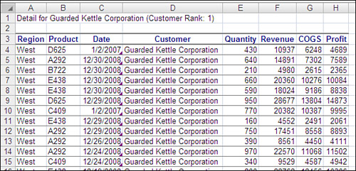
Example 13.10. Code Used to Create a Report for Each of the Top 3 Customers
Sub RetrieveTop3CustomerDetail()
    ' Listing 13.10
    ' Retrieve Details from Top 3 Stores
    Dim WSD As Worksheet
    Dim WSR As Worksheet
    Dim WBN As Workbook
    Dim PTCache As PivotCache
    Dim PT As PivotTable
    Dim PRange As Range
    Dim FinalRow As Long
    Set WSD = Worksheets("PivotTable")

    ' Delete any prior pivot tables
    For Each PT In WSD.PivotTables
        PT.TableRange2.Clear
    Next PT
    WSD.Range("J1:Z1").EntireColumn.Clear

    ' Define input area and set up a Pivot Cache
    FinalRow = WSD.Cells(Application.Rows.Count, 1).End(xlUp).Row
    FinalCol = WSD.Cells(1, Application.Columns.Count). _
        End(xlToLeft).Column
    Set PRange = WSD.Cells(1, 1).Resize(FinalRow, FinalCol)
    Set PTCache = ActiveWorkbook.PivotCaches.Add(SourceType:= _
        xlDatabase, SourceData:=PRange.Address)

    ' Create the Pivot Table from the Pivot Cache
    Set PT = PTCache.CreatePivotTable(TableDestination:=WSD. _
        Cells(2, FinalCol + 2), TableName:="PivotTable1")

    ' Turn off updating while building the table
    PT.ManualUpdate = True

    ' Set up the row fields
    PT.AddFields RowFields:="Customer", ColumnFields:="Data"

    ' Set up the data fields
    With PT.PivotFields("Revenue")
        .Orientation = xlDataField
        .Function = xlSum
        .Position = 1
        .NumberFormat = "#,##0"
        .Name = "Total Revenue"
    End With

    ' Sort Stores descending by sum of revenue
    PT.PivotFields("Customer").AutoSort Order:=xlDescending, _
        Field:="Total Revenue"

    ' Show only the top 3 stores
    PT.PivotFields("Customer").AutoShow Type:=xlAutomatic, Range:=xlTop, _
        Count:=3, Field:="Total Revenue"

    ' Ensure that we get zeros instead of blanks in the data area
    PT.NullString = "0"

    ' Calc the pivot table to allow the date label to be drawn
    PT.ManualUpdate = False
    PT.ManualUpdate = True

    ' Produce summary reports for each customer
    For i = 1 To 3
        PT.TableRange2.Offset(i + 1, 1).Resize(1, 1).ShowDetail = True
        ' The active sheet has changed to the new detail report
        ' Add a title
        Range("A1:A2").EntireRow.Insert
        Range("A1").Value = "Detail for " & _
            PT.TableRange2.Offset(i + 1, 0).Resize(1, 1).Value & _
            " (Customer Rank: " & i & ")"
    Next i

    MsgBox "Detail reports for top 3 customers have been created."
End SubA pivot table can have one or more Report Filter fields. A Report Filter field goes in a separate set of rows above the pivot report. It can serve to filter the report to a certain region, certain model, or certain combination of region and model.
In VBA, Report Filter fields are called page fields.
To set up a page field in VBA, add the PageFields parameter to the AddFields method. The following line of code creates a pivot table with Region in the page field:
PT.AddFields RowFields:= "Product", ColumnFields:= "Data", PageFields:= "Region"
The preceding line of code sets up the Region page field with the value (All), which returns all regions. To limit the report to just the North region, use the CurrentPage property:
PT.PivotFields("Region").CurrentPage = "North"One use of a page field is to build a user form in which someone can select a particular region or particular product. You then use this information to set the CurrentPage property and display the results of the user form.
Another interesting use is to loop through all PivotItems and display them one at a time in the page field. You can quickly produce top 10 reports for each region using this method.
To determine how many regions are available in the data, use PT.PivotFields("Region").PivotItems.Count. Either of these loops would work:
For i = 1 To PT.PivotFields("Region").PivotItems.Count
    PT.PivotFields("Region").CurrentPage = _
            PT.PivotFields("Region").PivotItems(i).Name
    PT.ManualUpdate = False
    PT.ManualUpdate = True
Next i

For Each PivItem In PT.PivotFields("Region").PivotItems
    PT.PivotFields("Region").CurrentPage = PivItem.Name
    PT.ManualUpdate = False
    PT.ManualUpdate = True
Next PivItem
Of course, in both of these loops, the three region reports fly by too quickly to see. In practice, you would want to save each report while it is displayed.
So far in this chapter, you have been using PT.TableRange2 when copying the data from the pivot table. The TableRange2 property includes all rows of the pivot table, including the page fields. There is also a .TableRange1 property, which excludes the page fields. You can use either statement to get the detail rows:
PT.TableRange2.Offset(3, 0)
PT.TableRange1.Offset(1, 0)
Which you use is your preference; but if you use TableRange2, you won’t have problems when you try to delete the pivot table with PT.TableRange2.Clear. If you were to accidentally attempt to clear TableRange1 when there are page fields, you would end up with the dreaded “Cannot move or change part of a pivot table” error.
Listing 13.11 produces a new workbook for each region. The report for the final region is shown in Figure 13.28.
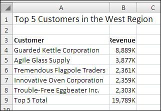
Example 13.11. Code That Creates a New Workbook per Region
Sub Top5ByRegionReport()
    ' Listing 13.11
    ' Produce a report of top 5 Customers for each region
    Dim WSD As Worksheet
    Dim WSR As Worksheet
    Dim WBN As Workbook
    Dim PTCache As PivotCache
    Dim PT As PivotTable
    Dim PRange As Range
    Dim FinalRow As Long

    Set WSD = Worksheets("PivotTable")

    ' Delete any prior pivot tables
    For Each PT In WSD.PivotTables
        PT.TableRange2.Clear
    Next PT
    WSD.Range("J1:Z1").EntireColumn.Clear

    ' Define input area and set up a Pivot Cache
    FinalRow = WSD.Cells(Application.Rows.Count, 1).End(xlUp).Row
    FinalCol = WSD.Cells(1, Application.Columns.Count). _
        End(xlToLeft).Column
    Set PRange = WSD.Cells(1, 1).Resize(FinalRow, FinalCol)
    Set PTCache = ActiveWorkbook.PivotCaches.Add(SourceType:= _
        xlDatabase, SourceData:=PRange.Address)

    ' Create the Pivot Table from the Pivot Cache
    Set PT = PTCache.CreatePivotTable(TableDestination:=WSD. _
        Cells(2, FinalCol + 2), TableName:="PivotTable1")

    ' Turn off updating while building the table
    PT.ManualUpdate = True

    ' Set up the row fields
    PT.AddFields RowFields:="Customer", ColumnFields:="Data", _
        PageFields:="Region"

    ' Set up the data fields
    With PT.PivotFields("Revenue")
        .Orientation = xlDataField
        .Function = xlSum
        .Position = 1
        .NumberFormat = "#,##0,K"
        .Name = "Total Revenue"
    End With

    ' Sort customers descending by sum of revenue
    PT.PivotFields("Customer").AutoSort Order:=xlDescending, _
        Field:="Total Revenue"

    ' Show only the top 5 customers
    PT.PivotFields("Customer").AutoShow Type:=xlAutomatic, Range:=xlTop, _
        Count:=5, Field:="Total Revenue"

    ' Ensure that we get zeros instead of blanks in the data area
    PT.NullString = "0"

    ' Calc the pivot table
    PT.ManualUpdate = False
    PT.ManualUpdate = True
    Ctr = 0

    ' Loop through each region
    For Each PivItem In PT.PivotFields("Region").PivotItems
        Ctr = Ctr + 1
        PT.PivotFields("Region").CurrentPage = PivItem.Name
        PT.ManualUpdate = False
        PT.ManualUpdate = True

        ' Create a new blank workbook with one worksheet
        Set WBN = Workbooks.Add(xlWBATWorksheet)
        Set WSR = WBN.Worksheets(1)
        WSR.Name = PivItem.Name
        ' Set up Title for Report
        With WSR.[A1]
            .Value = "Top 5 Customers in the " & PivItem.Name & " Region"
            .Font.Size = 14
        End With

        ' Copy the pivot table data to row 3 of the report sheet
        ' Use offset to eliminate the page & title rows of the pivot table
        PT.TableRange2.Offset(3, 0).Copy
        WSR.[A3].PasteSpecial Paste:=xlPasteValuesAndNumberFormats
        LastRow = WSR.Cells(65536, 1).End(xlUp).Row
        WSR.Cells(LastRow, 1).Value = "Top 5 Total"

        ' Do some basic formatting
        ' Autofit columns, bold the headings, right-align
        WSR.Range(WSR.Range("A2"), WSR.Cells(LastRow, 3)).Columns.AutoFit
        Range("A3").EntireRow.Font.Bold = True
        Range("A3").EntireRow.HorizontalAlignment = xlRight
        Range("A3").HorizontalAlignment = xlLeft
        Range("B3").Value = "Revenue"

        Range("A2").Select

    Next PivItem

    ' Clear the pivot table
    PT.TableRange2.Clear
    Set PTCache = Nothing

    MsgBox Ctr & " Region reports have been created"

End Sub
In addition to setting up a calculated pivot item to display the total of a couple of products that make up a dimension, you can manually filter a particular pivot field.
For example, you have one client who sells shoes. In the report showing sales of sandals, he wants to see just the stores that are in warm-weather states. The code to hide a particular store is as follows:
PT.PivotFields("Store").PivotItems("Minneapolis").Visible = FalseYou need to be very careful never to set all items to False; otherwise, the macro ends with an error. This tends to happen more than you would expect. An application might first show products A and B and then on the next loop show products C and D. If you attempt to make A and B not visible before making C and D visible, no products will be visible along the PivotField, which causes an error. To correct this, always loop through all PivotItems, making sure to turn them back to visible before the second pass through the loop.
This process is easy in VBA. After building the table with Product in the page field, loop through to change the Visible property to show only the total of certain products:
' Make sure all PivotItems along line are visible
For Each PivItem In _
    PT.PivotFields("Product").PivotItems
    PivItem.Visible = True
Next PivItem

' Now - loop through and keep only certain items visible
For Each PivItem In _
    PT.PivotFields("Product").PivotItems
    Select Case PivItem.Name
        Case "Landscaping/Grounds Care", _
            "Green Plants and Foliage Care"
            PivItem.Visible = True
        Case Else
            PivItem.Visible = False
    End Select
Next PivItemIf your company has been reporting regions in the sequence East, Central, West forever, it is an uphill battle getting managers to accept seeing the report ordered Central, East, West just because this is the default alphabetic order offered by pivot tables.
Strangely enough, Microsoft offers a bizarre method for handling a custom sort order in a pivot table. It’s called a manual sort order. To change the sort order in the user interface, you just go to a cell in the pivot table that contains Central, type the word East, and press Enter. As if by magic, Central and East switch places. Of course, all the numbers for East move to the appropriate column.
The VBA code to do a manual sort involves setting the Position property for a specific PivotItem. This is somewhat dangerous because you don’t know whether the underlying fields will have data for East on any given day. Be sure to set error checking to resume in case East doesn’t exist today:
On Error Resume Next
PT.PivotFields("Region").PivotItems("East").Position = 1
On Error GoTo 0So far, every example in this chapter has involved summing data. It is also possible to get an average, minimum, or maximum of data. In VBA, change the Function property of the Data field and give the Data field a unique name. For example, the following code fragment produces five different summaries of the Revenue field, each with a unique name:
' Set up the data fields
With PT.PivotFields("Revenue")
    .Orientation = xlDataField
    .Function = xlSum
    .Position = 1
    .NumberFormat = "#,##0,K"
    .Name = "Total Revenue"
End With

With PT.PivotFields("Revenue")
    .Orientation = xlDataField
    .Function = xlCount
    .Position = 2
    .NumberFormat = "#,##0"
    .Name = "Number Orders"
End With

With PT.PivotFields("Revenue")
    .Orientation = xlDataField
    .Function = xlAverage
    .Position = 3
    .NumberFormat = "#,##0"
    .Name = "Average Revenue"
End With

With PT.PivotFields("Revenue")
    .Orientation = xlDataField
    .Function = xlMin
    .Position = 4
    .NumberFormat = "#,##0"
    .Name = "Smallest Order"
End With

With PT.PivotFields("Revenue")
    .Orientation = xlDataField
    .Function = xlMax
    .Position = 5
    .NumberFormat = "#,##0"
    .Name = "Largest Order"
End With
The resultant pivot table provides a number of statistics about the average revenue, largest order, smallest order, and so on, as shown in Figure 13.29.

In addition to the available choices, such as Sum, Min, Max, and Average, you can use another set of pivot table options called the calculation options. They allow you to show a particular field as a percentage of the total, a percentage of the row, a percentage of the column, or as the percent difference from the previous or next item. All these settings are controlled through the .Calculation property of the page field.
The valid properties for .Calculation are xlPercentOf, xlPercentOfColumn, xlPercentOfRow, xlPercentOfTotal, xlRunningTotal, xlPercentDifferenceFrom, xlDifferenceFrom, xlIndex, and xlNoAdditionalCalculation. Each has its own unique set of rules. Some require that you specify a BaseField, and others require that you specify both a BaseField and BaseItem. The following sections provide some specific examples.
To get the percentage of the total, specify xlPercentOfTotal as the .Calculation property for the page field:
' Set up a percentage of total
With PT.PivotFields("Revenue")
    .Orientation = xlDataField
    .Caption = "PctOfTotal"
    .Function = xlSum
    .Position = 2
    .NumberFormat = "#0.0%"
    .Calculation = xlPercentOfTotal
End WithWith ship months going down the columns, you might want to see the percentage of revenue growth from month to month. You can set up this arrangement with the xlPercentDifferenceFrom setting. In this case, you must specify that the BaseField is "Date" and that the BaseItem is something called (previous):
' Set up % change from prior month
With PT.PivotFields("Revenue")
    .Orientation = xlDataField
    .Function = xlSum
    .Caption = "%Change"
    .Calculation = xlPercentDifferenceFrom
    .BaseField = "Date"
    .BaseItem = "(previous)"
    .Position = 3
    .NumberFormat = "#0.0%"
End With
Note that with positional calculations, you cannot use the AutoShow or AutoSort method. This is too bad; it would be interesting to sort the customers high to low and to see their sizes in relation to each other.
You can use the xlPercentDifferenceFrom setting to express revenues as a percentage of the West region sales:
' Show revenue as a percentage of California
With PT.PivotFields("Revenue")
    .Orientation = xlDataField
    .Function = xlSum
    .Caption = "% of West"
    .Calculation = xlPercentDifferenceFrom
    .BaseField = "Region"
    .BaseItem = "West"
    .Position = 3
    .NumberFormat = "#0.0%"
End WithSetting up a running total is not intuitive; to do this, you must define a BaseField. In this example, Date runs down the column. To define a running total column for revenue, you must specify that BaseField is "Date":
' Set up Running Total
With PT.PivotFields("Revenue")
    .Orientation = xlDataField
    .Function = xlSum
    .Caption = "YTD Total"
    .Calculation = xlRunningTotal
    .Position = 4
    .NumberFormat = "#,##0,K"
    .BaseField = "Date"
End With
Figure 13.30 shows the results of a pivot table with three custom calculation settings, as discussed earlier.

Pivot tables offer a variety of new features in Excel 2007. The new label and value filters, conditional formatting, table formatting, and layout views are significant improvements to the pivot table environment.
If you want to use any of these features, the pivot table must exist in a file stored in Excel 2007 file format. If your file is in Compatibility mode, none of the new features are available in the user interface or in VBA.
Similarly, if you use any of these features, the code runs only in Excel 2007. There is no hope of going backward to share the code with someone using Excel 2003.
In previous versions of Excel, the filtering feature enabled you to choose one or more pivot items from a drop-down list. The only conceptual filter was the top 10 AutoShow filter.
Excel 2007 offers new conceptual filters that are easy to access. In the PivotTable Field List, hover the cursor over any active field in the field list portion of the dialog box. In the drop-down that appears, you can choose Label Filters, Date Filters, or Value Filters.
In Figure 13.31, the fly-out menu shows the list of Label filters available for the Customer field.
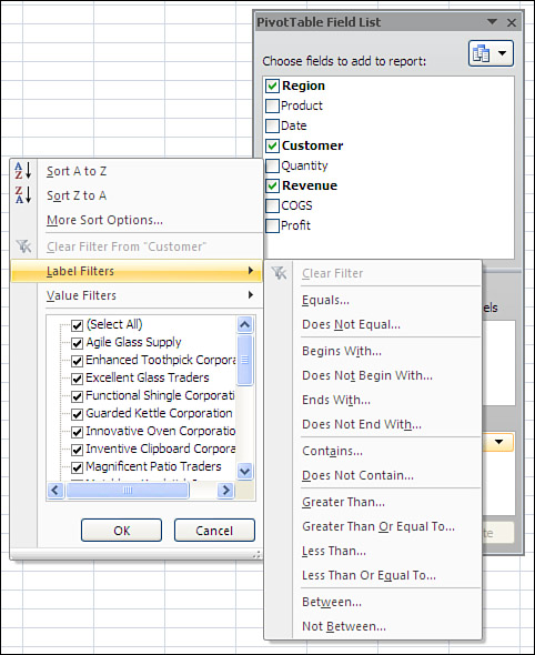
To apply a label filter in VBA, use the PivotFilters.Add method. The following code filters to the branches that start with 1:
PT.PivotFields("Customer").PivotFilters.Add _
    Type:=xlCaptionBeginsWith, Value1:="1"
To clear the filter from the Branch field, use the ClearAllFilters method:
PT.PivotFields("Customer").ClearAllFiltersTo apply a date filter to the Date field to find records from this week, use this code:
PT.PivotFields("Date").PivotFilters.Add Type:=xlThisWeekThe value filters enable you to filter one field based on the value of another field. For example, to find all the branches where the total revenue is more than $100,000, you would use this code:
PT.PivotFields("Customer").PivotFilters.Add _
    Type:=xlValueIsGreaterThan, _
    DataField:=PT.PivotFields("Sum of Revenue"), _
    Value1:=100000
Other value filters might allow you to specify that you want branches where the revenue is between $50,000 and $100,000. In this case, you specify one limit as Value1 and the second limit as Value2:
PT.PivotFields("Branch").PivotFilters.Add _
    Type:=xlValueIsBetween, _
    DataField:=PT.PivotFields("Sum of Revenue"), _
    Value1:=50000, Value2:=100000
Table 13.3 provides a sampling of filter types.
Table 13.3. Sampling of Filter Types
Description | |
|---|---|
| Filters for all dates before a specified date |
| Filters for all dates in January |
| Filters for the specified number of values from the bottom of a list |
| Filters for the specified percentage of values from the bottom of a list |
| Sums the values from the bottom of the list |
| Filters for all captions beginning with the specified string |
| Filters for all dates that are between a specified range of dates |
| Filters for all dates that apply to the previous month |
| Filters for all values that match the specified value |
| Filters for all values that are within one year of a specified date |
The Design ribbon offers two groups dedicated to formatting the pivot table, as shown in Figure 13.32. The PivotTable Style Options group has four check boxes that modify the styles in the PivotTable Styles Gallery.
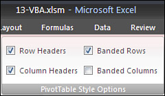
The following four lines of code are equivalent to turning on all four settings in the PivotTable Style Options group:
PT.ShowTableStyleRowHeaders = True
PT.ShowTableStyleColumnHeaders = True
PT.ShowTableStyleRowStripes = True
PT.ShowTableStyleColumnStripes = True
To apply a table style from the gallery, use the TableStyle2 property. If you want to get the correct name, it might be best to record a macro:
' Format the pivot table
PT.ShowTableStyleRowStripes = True
PT.TableStyle2 = "PivotStyleMedium3"
If you hover over a style in the Style gallery, a ToolTip will show a style name such as Pivot Style Medium 3.
The Layout group of the Design ribbon contains four drop-downs. These drop-downs control the location of subtotals (top or bottom), the presence of grand totals, the report layout, and the presence of blank rows.
Subtotals can appear either at the top or bottom of a group of pivot items. The SubtotalLocation property applies to the entire pivot table; valid values are xlAtBottom or xlAtTop:
PT.SubtotalLocation:=xlAtTop
Grand totals can be turned on or off for rows or columns. The following code turns them off for both:
PT.ColumnGrand = False
PT.RowGrand = False
There are three settings for the report layout. The Tabular layout is similar to the default layout in Excel 2003. The Outline layout was optionally available in Excel 2003. The Compact layout is new in Excel 2007.
Excel can remember the last layout used and apply it to additional pivot tables created in the same Excel session. For this reason, you should always explicitly choose the layout that you want. Use the RowAxisLayout method; valid values are xlTabularRow, xlOutlineRow, or xlCompactRow:
PT.RowAxisLayout xlTabularRow
PT.RowAxisLayout xlOutlineRow
PT.RowGrand = xlCompactRow
In Excel 2007, you can add a blank line to the layout after each group of pivot items. Although the Design ribbon offers a single setting to affect the entire pivot table, the setting is actually applied to each individual pivot field individually. The macro recorder responds by recording a dozen lines of code for a pivot table with 12 fields. You can intelligently add a single line of code for the outer Row field(s):
PT.PivotFields("Region").LayoutBlankLine = TrueApplying a Data Visualization
Excel 2007 offers fantastic new data visualizations such as icon sets, color gradients, and in-cell data bars. When you apply a visualization to a pivot table, you should exclude the total rows from the visualization.
If you have 20 customers that average $3,000,000 in revenue each, the total for the 20 customers is $60 million. If you include the total in the data visualization, the total gets the largest bar, and all the customer records have tiny bars.
In the Excel user interface, you always want to use the Add Rule or Edit Rule choice to choose the option All Cells Showing “Sum of Revenue” for “Customer,” as shown in Figure 13.33.

The code in Listing 13.12 adds a pivot table and applies a data bar to the revenue field.
Example 13.12. Code That Creates a Pivot Table with Data Bars
Sub Sub CreatePivotDataBar()
    ' Listing 13.12
    Dim WSD As Worksheet
    Dim PTCache As PivotCache
    Dim PT As PivotTable
    Dim PRange As Range
    Dim FinalRow As Long
    Set WSD = Worksheets("PivotTable")

    ' Delete any prior pivot tables
    For Each PT In WSD.PivotTables
        PT.TableRange2.Clear
    Next PT
    WSD.Range("J1:Z1").EntireColumn.Clear

    ' Define input area and set up a Pivot Cache
    FinalRow = WSD.Cells(Rows.Count, 1).End(xlUp).Row
    FinalCol = WSD.Cells(1, Columns.Count). _
        End(xlToLeft).Column
    Set PRange = WSD.Cells(1, 1).Resize(FinalRow, FinalCol)
    Set PTCache = ActiveWorkbook.PivotCaches.Add(SourceType:= _
        xlDatabase, SourceData:=PRange.Address)

    ' Create the Pivot Table from the Pivot Cache
    Set PT = PTCache.CreatePivotTable(TableDestination:=WSD. _
        Cells(2, FinalCol + 2), TableName:="PivotTable1")

    ' Turn off updating while building the table
    PT.ManualUpdate = True

    ' Set up the row & column fields
    PT.AddFields RowFields:="Customer", _
        ColumnFields:="Data"

    ' Set up the data fields
    With PT.PivotFields("Revenue")
        .Orientation = xlDataField
        .Function = xlSum
        .Position = 1
    End With

    ' Calc the pivot table
    PT.ManualUpdate = False
    PT.ManualUpdate = True

    ' Apply a Databar
    PT.TableRange2.Cells(3, 2).Select
    Selection.FormatConditions.AddDatabar
    Selection.FormatConditions(1).ShowValue = True
    Selection.FormatConditions(1).SetFirstPriority
    With Selection.FormatConditions(1)
        .MinPoint.Modify newtype:=xlConditionValueLowestValue
        .MaxPoint.Modify newtype:=xlConditionValueHighestValue
    End With
    With Selection.FormatConditions(1).BarColor
        .ThemeColor = xlThemeColorAccent3
        .TintAndShade = -0.499984740745262
    End With
    Selection.FormatConditions(1).ScopeType = xlFieldsScope

    WSD.Activate
    Range("J2").Select

End SubIf you couldn’t already tell, pivot tables are my favorite feature in Excel. They are incredibly powerful and flexible. Combined with VBA, they provide an excellent calculation engine and power many of the reports that I build for clients. In Chapter 14, “Excel Power,” you will learn multiple techniques for handling various tasks in VBA.