Chapter 9 SAS/GRAPH Elements You Should Know—Even if You Don’t Use SAS/GRAPH

9.1 Using Title Options with ODS

9.2 Setting and Clearing Graphics Options and Settings

9.3 Using SAS/GRAPH Statements with Procedures That Are Not SAS/GRAPH Procedures

9.3.1 Changing Plot Symbols with the SYMBOL Statement

9.3.2 Controlling Axes and Legends

9.4 Using ANNOTATE to Augment Graphs

The Output Delivery System, ODS, gives us a great deal of the kind of control that we must have in order to produce the kinds of reports and tables that are expected of us. Although we will often include graphical elements in our tables, it turns out that a number of options, statements, and techniques that are associated with SAS/GRAPH can be utilized to our benefit even when we are NOT creating graphs. In this chapter you will learn how to take advantage of these graphical elements even when you are not using SAS/GRAPH.

Some of the options and statements described in this chapter are not available if your site has not licensed SAS/GRAPH. If SAS/GRAPH is not available to you, try to get your site to license it; otherwise, experiment. A lot of the things shown in this chapter will work anyway, but not everything!

SEE ALSO

Carpenter (2010b) contains a number of other related examples.

9.1 Using Title Options with ODS

For destinations that support font and color attributes, the Output Delivery System, ODS, honors many of the SAS/GRAPH title and footnote options.

A few of the traditional TITLE/FOOTNOTE statement options include:

Most of these options can be abbreviated. For the options shown above, you can use the uppercase letters in the option name as an abbreviation.

There are also a few font modification options. These include:

Colors can include most standard color names as well as any of the RGB or gray-scale colors that are appropriate for the output destination.

These options are listed in the Base SAS TITLE statement documentation, as well as in the SAS/GRAPH documentation; however, a number of the SAS/GRAPH TITLE statement options are not supported outside of the graphics environment. The following example demonstrates some of these TITLE statement options using titles associated with an RTF report.

title1  f='times new roman' 

        h=15pt c=blue 

        bc=yellow 

        '9.1a Using TITLE Options';

ods rtf file="&path
esultsE9_1a.rtf"

        style=rtf;

title2 f='Arial' h=13pt c=red 

       j=l 

       bold 

       'English Units';

proc report data=advrpt.demog nowd split='*';

. . . portions of the REPORT step are not shown . . . .

You may use any font available to your system. Fonts consisting of more than one word must be enclosed in quotation marks.

The font size is set to 15 points. This can be a fairly nominal size, as actual size can depend on the destination and how it is displayed.

The background color is set to yellow.

JUSTIFY=LEFT has been abbreviated.

The font is boldfaced.

RTF

PDF

HTML

When using the RTF style in the RTF destination, changing the background color (BC=) adds a box around the title.

In RTF, by default, the titles and footnotes are added to the HEADER and FOOTERS of the document when the table is imported. Footers are at the bottom of the physical page, and not necessarily at the bottom of the table. The titles/footnotes can be made a part of the table itself through the use of the BODYTITLE option. For shorter tables this can move the footnote to the base of the table.

title1 '9.1c Horizontal Lines';

title2  h=5pt bcolor=blue ' '; 

footnote h=5pt bcolor=blue ' '; 

ods html file="&path
esultsE9_1c.html";

proc print data=sashelp.class(obs=4);

run;

ods html close;

ods rtf file="&path
esultsE9_1b.rtf"

        style=rtf

        bodytitle;

Through the use of the background color option (BCOLOR) you can change the color behind the title’s text. This option can also be used to create colorful horizontal lines. The BCOLOR option specifies the background color. Some text, if only a blank space, must be specified.

There are quite a few other SAS/GRAPH TITLE statement options. Most of these options are ignored outside of SAS/GRAPH. Depending on the destination and style, some SAS/GRAPH TITLE statement options are occasionally not ignored (when you think that they should be). In these cases they tend to yield unanticipated results.

SEE ALSO

The horizontal lines example originated from a tip supplied by Don Henderson on sasCommunity.org at http://www.sascommunity.org/wiki/Tip_of_the_Day:April_26.

TITLE / FOOTNOTE options are also documented at http://support.sas.com/documentation/cdl/en/lrdict/64316/HTML/default/viewer.htm#a000220968.htm (see Example 3 for specific usages of these options).

9.2 Setting and Clearing Graphics Options and Settings

Most procedures that have graphics capabilities can also take advantage of many graphics options and settings. Not all of the graphics options will be utilized outside of the SAS/GRAPH environment, so you may need to do some experimenting to determine which graphics options are used for your OS, version of SAS, ODS destination, and the procedure of interest.

Graphics options are set through the use of the GOPTIONS statement. Like the OPTIONS statement, this global statement is used to set one or more graphics options. Because there are a great many aspects to the preparation and presentation of a high-resolution graphic, there are necessarily a large number of graphics options.

A few of the more commonly used options are shown here.

Because these options and settings have a scope for the entire session, if you are in an interactive session and execute two or more programs that use or change some of these options, it is not uncommon to have the options from one program interfere with the options of the next program. You can mitigate this interference by setting or resetting the options to their default values at the start of each program by using the RESET= option.

goptions reset=symbol;

The RESET= graphics option can be used to reset a number of different groups of graphic settings. The following table shows some of these groups.

The following is a rather typical set of GOPTION statements.

FILENAME fileref "&path
esultsFinalReport.emf";

goptions reset=all border 

         ftext=simplex; 

GOPTIONS GSFNAME=fileref  GSFMODE=replace 

         DEVICE=emf; 

*goptions device=win 

         targetdevice=emf; 

The RESET=all option clears all graphics options and sets them to their default values. Borders around the graphs are then turned on.

The FTEXT= option is used to set the default font for graphics text. SIMPLEX is similar to ARIAL; however, this SAS/GRAPH font may not be available if your site does not license SAS/GRAPH.

Graphics Stream File options, GSF, are used to route the graph to a file.

• GSFNAME= points to the destination of the graphic (in this case a fileref named FILEREF).
• GSFMODE= if the graphic file already exists, REPLACE indicates that the graphic is to be replaced.

The DEVICE= option is used to structure the graph for the appropriate physical or virtual destination. EMF is a good device when the graphic is to be included in a word processing document.

During program development you will want to see the graph displayed on the monitor (DEVICE=WIN); however, you may want to view it as it will ultimately be displayed on the final destination. The TARGETDEVICE= option attempts to show you the graph on the display device (DEVICE=) using the constraints of the eventual final device (TARGETDEVICE=). In this production example this development statement has been commented out.

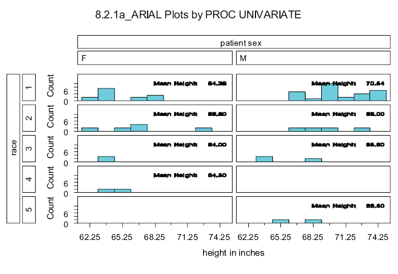
FTEXT= can be especially important when generating graphics using procedures such as PROC UNIVARIATE. In the example plot appearing in Section 8.2.1a, and shown here as well, some of the text is virtually unreadable. This can be a result of the automatic default selection of hardware fonts that do not scale appropriately. The FTEXT= option can be used to specify the default font. The only coding changes between these two versions of this graphic is the use of the FTEXT= option. Notice that there are several changes including text orientation as well as readability. Note that the font used on the interior graphics was not changed.

goptions device=emf  

         ftext=arial 

         gsfname=out821a 

         noprompt;

When these options are being used with ODS you may want to control whether or not they should override the selected style. Starting in SAS 9.2 the application of some of these options can be restricted with the use of the ODS USEGOPT statement. When USEGOPT is in effect, the settings for the following graphics options will take precedence over the ODS style and will affect all of your ODS output, including tables as well as graphics GOPTIONS. Affected graphics options include:

FTEXT=, CTEXT=, HTEXT=, FTITLE=, CTITLE=, HTITLE=.

When ODS NOUSEGOPT is in effect, the settings for these graphics options will not override the value in the style definition in your ODS output.

MORE INFORMATION

Although not generally shown in the code included in the text of this book, graphics options are used in examples throughout Chapters 9 and 10. Examine the sample code for more examples of the use of graphics options.

9.3 Using SAS/GRAPH Statements with Procedures That Are Not SAS/GRAPH Procedures

There are a number of other procedures that although not part of SAS/GRAPH are none-the-less able to take advantage of SAS/GRAPH statements when generating high-resolution graphs.

A few of the more common procedures that I have found to be useful that also have high-resolution graphics capabilities include:

Base

PROC UNIVARIATE (see Section 8.2)

SAS/QC

PROC CAPABILITY

PROC SHEWART (see Section 10.1.3)

SAS/STAT

PROC BOXPLOT (see Section 10.1.1)

PROC PROBIT

PROC REG

The remainder of this section is a very brief introduction to some of the statements that can be used outside of SAS/GRAPH. Better and more complete introductions to SAS/GRAPH can be found in numerous papers, as well as in several books.

CAVEAT

If you do not have access to SAS/GRAPH and depending on your release of SAS, some of the techniques and capabilities described in this section may not be available to you. This is true even if you are not using a SAS/GRAPH procedure.

MORE INFORMATION

The probability and QQ plots generated by PROC UNIVARIATE in Section 8.2.3 can take advantage of the SYMBOL statement (see Section 9.3.1).

Section 9.1 demonstrates the use of SAS/GRAPH options in TITLE and FOOTNOTE statements as they can be applied to output generated by the Output Delivery System.

SEE ALSO

Books that specifically provide introductions to SAS/GRAPH include Carpenter and Shipp (1995), Carpenter (1999), and Miron (1995).

9.3.1 Changing Plot Symbols with the SYMBOL Statement

The SYMBOL statement is used to control the appearance of items within the graphics area. As you would suspect this includes plot symbols, but it also controls the appearance of lines, and how points are joined with these lines. All plot symbols and lines have attributes, e.g., color, size, shape, thickness. These attributes are all controlled with the SYMBOL statement.

There can be up to 99 numbered SYMBOL statements. Attributes to be controlled are specified through the use of options. Options are specified through the use of their names and, in most cases, the names can be abbreviated. This SYMBOL statement requests that the plot symbols (a dot) be blue, with a size (height) of .8 units.

symbol1 color = blue h = .8 v=dot;

Fortunately, since the SYMBOL statement is heavily used, it is usually fairly straightforward to apply. A quick study of the documentation will usually serve as a first pass instruction. Like so many things in SAS however, there are a few traps that you should be aware of when applying the SYMBOL statement in more complex situations.

A few of the numerous SYMBOL statement options are shown in the following table.

SYMBOL Definitions Are Cumulative

Although SYMBOL statements, like TITLE and FOOTNOTE statements, are numbered, that is about the only similarity with regard to the way that the definitions are established. When a TITLE3 statement is specified, the definition for TITLE3 is completely replaced. Not only is a given TITLE statement the complete definition for that title, but that same TITLE3 statement automatically clears titles 4 through 10. SYMBOL statement definitions, on the other hand, are cumulative, and each numbered statement is independent of statements with other numbers.

The two SYMBOL statements on the left could be rewritten as a series of statements.

symbol1 color = blue v=none 

        i=box10 bwidth=3;

symbol2 color = red  v=dot 

        i=join line=2 h=1.2;

symbol2 v=dot  i=join;

symbol1 color = blue; 

symbol2 color = red;  

symbol1 v=none i=box10 bwidth=3;

symbol2 line=2 h=1.2;

The graphics option RESET can be used in the GOPTIONS statement to clear SYMBOL statement definitions.

goptions reset=symbol;

SYMBOL Definition Selection Is NOT User Directed

When symbols or lines are to be used in a graph, the procedure first checks to see if there are any user defined symbol definitions (of course, there are defaults for everything when SYMBOL statements have not been used). The procedure then selects the next available symbol definition. This means that if SYMBOL2 was just used, the procedure will look for a SYMBOL3 definition.

Unfortunately it is not generally possible to directly tie a given symbol statement to a given line or symbol. This means that you will need to have at least a basic understanding of symbol definition selection for the procedure that you are planning on using.

The following example uses PROC REG to perform a regression analysis on HT and WT in the DEMOG data set. The PLOT statement can be used to create a plot of the results of the analysis.

goptions reset=all; 

title1 f=arial bold 'Regression of HT and WT'; 

title2 '9.3.1a No SYMBOL Statement';

proc reg data=advrpt.demog;

model ht = wt; 

plot ht*wt/conf; 

run;

quit;

All graphics options are set to their defaults.

TITLE statement options are used to select boldface ARIAL as the font for the first title.

HT is used as the dependent variable.

The CONF option is used to request the plotting of the confidence intervals and predicted values.

Although the procedure selects colors and line types for the predicted value line and for the confidence intervals, the data is plotted using the plus ‘+’ symbol.

We can use the SYMBOL statement to gain control of the plot symbol.

title2 '9.3.1b With SYMBOL Statements';

symbol1 c=blue  v=dot; 

symbol2 c=red; 

symbol3 c=green r=2; 

For the data points, the SYMBOL1 statement is used to select the plot symbol attributes. In this case the color and the symbol (V=).

The color for the estimated line is specified. You will need to experiment to determine which SYMBOL statement will be used by which aspect of the graph.

The confidence lines are colored green. The R= option causes this symbol definition to be reused a second time. Otherwise, we could have specified the SYMBOL4 definition to be the same as the SYMBOL3 definition.

The colors and plot symbols are shown in the legend at the bottom of the graph. You can take control of the legend though the use of the LEGEND statement (see Section 9.3.2). Although not supported by PROC REG, for some procedures you can eliminate the legend altogether using the NOLEGEND option.

9.3.2 Controlling Axes and Legends

Control of any and all aspects of the horizontal and vertical axes can be obtained through the use of the AXIS statement. This global statement can be one of the most complex statements in SAS/GRAPH, if not within SAS itself, and it is clearly outside of the scope of this book to do much more than just partially describe this statement. Closely related to the AXIS statement in syntax is the LEGEND statement, which is used to control the appearance of the graph’s legend. The following is a brief introduction to these two statements.

Like the SYMBOL statement, you can have up to 99 numbered AXIS and LEGEND statements. Also like the SYMBOL statement, the axis and legend definitions are cumulative. Both axis and legend definitions can be cleared with the RESET= option.

goptions reset=axis;

goptions reset=legend;

AXIS Statement

The AXIS statement can be used to control the axis lines, tick marks, tick mark text, and axis labels.

You can specify fonts and color for all text. For any of the lines you can control the styles (type of line), thickness, color, and length.

The axis definition is built through a series of options. Some of these options will themselves have options, and the layers of options with options can often be three deep. To make things even more interesting, some options will appear in multiple ways and their effect will depend on position and usage. Clearly just knowing how to apply the options and how to nest them can be complicated.

Most of the options that can appear in several different aspects of the statement are text appearance options. Most options are similar to those used as TITLE and FOOTNOTE statement options (see Section 9.1), and there is also some overlap with those options used in the SYMBOL statement. Some of the more common text appearance options include:

The first layer of options control major aspects of the axis. These include such things as:

• ORDER= range of values to be included
• LABEL= axis label
• VALUE= tick mark control
• MAJOR= major tick marks (the ones with text)
• MINOR= minor tick marks

When building an AXIS statement, parentheses are used to form groups of sub-options, and indenting to each level of option can be helpful in keeping track of which options go with what. This is a fairly typical AXIS statement. Notice that the values of options are in parentheses. This allows you to specify the sub-options.

axis2 order =(3 to 6 by 1) 

      label =(h=2 

              font='Times New Roman' 

              "Potassium Levels") 

      minor =(n=1) 

             angle=90 

             rotate=0  ; 

axis1 minor=(n=4)   

      color=black

      label=( "BMI")

      order=(15 to 40 by 5);

ORDER= Restricts the axis range; data can be excluded. Here the range of the axis is limited to values between 3 and 6 with major tick marks at the integers. The VALUE= option (shown in the LEGEND example) specifies the attributes of the major tick marks.

H= sets the height of the label’s text to 2 units (the default units are cells).

FONT= specifies the font. Fonts with multiple words should be quoted.

‘text’ specifies the text for the label, which overrides the variable’s label.

MINOR= specifies the number of minor tick marks. The keyword NONE can be used to turn off minor tick marks.

ANGLE= rotates the entire label 90 degrees (from horizontal to vertical). Angle=0 is horizontal.

ROTATE= rotates the letters within the line of text individually.

proc gplot data=bmi;

   plot potassium*bmi/haxis=axis1 

                      vaxis=axis2;

   run;

The individual AXIS definitions are assigned to an axis on the plot or graphic through options on the PLOT statement.

LEGEND Statement

The general syntax, statement structure, and even many of the options of the AXIS statement are shared with the LEGEND statement. In the regression plots in Section 9.3.1, the legend appears at the bottom of the graph. We can change its location as well as its appearance.

legend1 position=(top left inside) 

        value=(f='arial' t=1 'Height' 

                         t=2 'Predicted'

                         t=3 'Upper 95'

                         t=4 'Lower 95')

        label=none 

        frame 

        across=2; 

proc reg data=advrpt.demog;

model ht = wt;

plot ht*wt/conf

           legend=legend1; 

run;

The legend can be INSIDE or OUTSIDE of the graphics area. It can also be moved vertically and horizontally.

The VALUE= option controls the text associated with the four individual items in the legend.

The LABEL=NONE option turns off the legend’s label.

The FRAME option adds a box around the legend. Other options allow you to change the width, color, and shadowing of the frame.

The ACROSS=2 option allows at most 2 items for each row in the legend.

The LEGEND= option identifies the appropriate legend statement.

For this graph, especially when displayed in black and white, the legend is fairly superfluous. Many procedures have an option (NOLEGEND) that can be used to prevent the display of the option. PROC REG does not support the NOLEGEND option. Consequently, there is no way to prevent the legend from appearing when any of the PLOT statement options that cause multiple items to be displayed (such as CONF) are used. The following example uses a LEGEND statement to minimize the impact of the legend.

legend2 value= none 

        label=none 

        shape=symbol(.001,.001); 

proc reg data=advrpt.demog;

model ht = wt;

plot ht*wt/conf

           legend=legend2; 

run;

The text for the individual values is turned off.

The label is turned off.

The individual symbol elements cannot be turned off (SHAPE does not support NONE); therefore, the values are made very small.

The LEGEND2 definition is selected for use.

MORE INFORMATION

The AXIS statement is used in an example in Section 10.1.1.

9.4 Using ANNOTATE to Augment Graphs

The annotate facility gives us the ability to customize the output generated by the procedure. The huge advantage is that the customization can be data dependent, without recoding. The key to the process is the annotate data set. This data set contains the instructions that are to be passed to the annotate facility. Each observation in the data set is one instruction, and very often the instruction is fairly primitive, e.g., pick up a pen.

The instructions in the data set are passed to the procedure that is generating the graphic through the use of the ANNOTATE= option. You can tell if a procedure can take advantage of the annotate facility when it supports this option or its abbreviation, which is ANNO=.

Since the annotate facility interprets each observation of the annotate data set as an instruction, it uses the values of specific variables to form the intent of the instruction. You do not get to choose the names of the variables, but you have a great deal to do with the values that the variables take on. In order for the instruction to provide a valid instruction to annotate, the variables and their values have to provide answers to three primary questions.

The value of the variable FUNCTION is always specified, and this value determines what other variables will be used by annotate when the instruction is executed. FUNCTION should be a character variable with a length of 8. There are over two dozen possible values for FUNCTION; three of the commonly used values are shown here.

Other commonly used annotate functions include tools for:

• generating polygons, bars, and pie slices
• drawing symbols, arrows, and lines
• including text and images

For annotate operations that are associated with a location on a graphic, variables are used to specify the location. In order to identify a location, you will need to specify the coordinate system (e.g., XSYS, YSYS) and a location within that coordinate system (e.g., X, Y).

In this example the Body Mass Index, BMI, is calculated and then added using the annotate facility to the regression plot generated by PROC REG (see Section 9.3).

data bmilabel(keep=function  

                   xsys ysys x y 

                   text color style 

                   position size);

   set advrpt.demog;

   * Define annotate variable attributes;

   length color function $8; 

   retain function 'label' 

          xsys ysys '2'

          color 'red'

          style 'arial'

          position '2'

          size .8;

   * Calculate the BMI. Note those outside of 

   * the range of 18 - 26;

   bmi = wt / (ht*ht) * 703; 

   if bmi lt 18 or bmi gt 26 then do; 

      * Create a label;

      text = put(bmi,4.1); 

      x=wt;

      y=ht;

      output bmilabel; 

   end;

   run;

The annotate data set is named (WORK.BMILABEL), and the variables that it will contain are specified.

The annotate variables FUNCTION and COLOR are assigned a length in order to avoid truncation. This is always a good idea.

The annotate variables that are constant for all the instructions (observations) are assigned values with the RETAIN.

Create an annotate instruction (a label) only for those observations with a BMI outside of the stated range.

The variables X and Y contain the coordinates of this data point on the graph. TEXT, the annotate label, contains the value of the variable BMI.

Write this annotate instruction to the annotate data set.

The ANNO= option is used to name the data set that contains the annotate instructions.

proc reg data=advrpt.demog;

   model ht = wt;

   plot ht*wt/conf legend=legend1

              anno=bmilabel; 

   run;

The BMI values that are outside of the selected range are added to the plot as annotate labels. The location of the label is based on the data values that are also used to generate the plot and the regression.

SEE ALSO

An introduction to the annotate facility can be found in Carpenter (1999).

Values can also be added to points using the SYMBOL statement option POINTLABEL. See
http://communities.sas.com/message/100627#100627.