The use of formats is essential to the process of analysis and reporting of data. The user must be well grounded not only in the basic application of formats, but the deeper, less commonly known aspects as well. The power of formats can be taken advantage of in a wide variety of situations. It is incumbent on the user that these capabilities are fully understood.

MORE INFORMATION

Section 3.5.1 discusses the difference between formats and informats and their uses in the conversion of character to numeric values.

12.1 Using Preloaded Formats to Modify Report Contents

Generally when a level of a classification variable is not included in the data, that level will not appear in any reports or analyses based on that data. Preloaded formats provide a mechanism to not only force the inclusion of those absent classification levels, they can also be used to filter or remove unwanted levels.

Preloaded formats can be used with the REPORT, TABULATE, MEANS and SUMMARY procedures. Preloaded formats are invoked through the use of options, and the available options and their usage varies for each procedure. For each procedure it is the interaction of these options that determines the resulting table. For the examples in this section study the results of the various combinations of the options, then experiment using other combinations.

For each of these procedures the two primary options used are PRELOADFMT and EXCLUSIVE:

PRELOADFMT	Loads the format levels prior to execution. This option will always be present when using preloaded formats.
EXCLUSIVE	Only data levels that are included in the format definition are to appear in table.

proc format;

   value $regx

      '1'=' 1'

      '2'=' 2'

      'X'=' X' ;

   value $genderu

      'M'='Male'

      'F'='Female'

      'U'='Unknown';

   value $symp

      '00'= 'Unspecified'

      '01'= 'Sleepiness'

      '02'= 'Coughing'

      '03'= 'Limping';

   run;

As the name implies preloaded formats key off of what is generally a user-defined format. The formats $REGX., $GENDERU., and $SYMP., which are defined here, are used in the examples that follow. Each contains one level that is not in the data , and both $REGX. and $SYMP. exclude levels that are found in the data. The format $REGX. is used with the variable REGION, which ranges from ‘1’ through ‘10’. The format $SYMP. is used with the variable SYMP, which ranges from ‘01’ through ‘10’. The format $GENDERU. is used with the variable SEX which takes on the values of ‘F’ and ‘M’.

12.1.1 Using Preloaded Formats with PROC REPORT

When preloading formats with the REPORT procedure, the PRELOADFMT and, if used, the EXCLUSIVE options are applied on the DEFINE statement.

In addition to the PRELOADFMT and EXCLUSIVE options, the REPORT procedure can also take advantage of the options COMPLETEROWS and COMPLETECOLS:

COMPLETEROWS	All rows representing format levels are to appear in the report.
COMPLETECOLS	All columns representing format levels are to appear in the report.

The following examples show various combinations of these options. Although they do not discuss the use of COMPLETECOLS, its behavior is similar to COMPLETEROWS, which is discussed here. This can be easily demonstrated by applying these options to the report item SEX in these same examples.

Remember that you must apply the PRELOADFMT option on the DEFINE statement for each report item for which you want to preload a format.

Using PRELOADFMT with EXCLUSIVE

Preloading with the EXCLUSIVE option allows only those levels that are on the format and in the data. In PROC REPORT these options are applied on the DEFINE statement.

title2 'Using PRELOADFMT with EXCLUSIVE';

proc report data=demog nowd;

   column region sex,(wt=n wt);

   define region / group

                   format=$regx6.

                   preloadfmt exclusive;

   define sex    / across        format=$Genderu. 'Gender';

   define n      / analysis n    format=2.0 'N';

   define wt     / analysis mean format=6.2 'Weight';

   run;

Using the format $REGX. along with these two options causes only regions 1 and 2 to appear in the report, as these are the only two regions that are both in the format and in the data.

12.1.1 Preloading Formats in PROC REPORT

Using PRELOADFMT with EXCLUSIVE

                  Gender

            Female       Male

  region   N  Weight   N  Weight

   1       .     .     4  195.00

   2       6  109.67   3  105.00

Using COMPLETEROWS without EXCLUSIVE

The COMPLETEROWS option, which is used on the PROC statement, forces all levels that appear either in the data or in the format to appear on the report.

title2 'Using COMPLETEROWS with PRELOADFMT and without EXCLUSIVE';

proc report data=demog nowd completerows;

   column region sex,(wt=n wt);

   define region / group format=$regx6.

                   preloadfmt

                   order=data;

   define sex    / across        format=$Genderu. 'Gender';

   define n      / analysis n    format=2.0 'N';

   define wt     / analysis mean format=6.2 'Weight';

   run;

In this example the ORDER=DATA option also appears on the DEFINE statement. Prior to SAS 9.2 the ORDER= option was expected, although not always required. Notice that all three format levels appear. Except for REGION ‘X’, which does not appear in the data, the output is now in data order (the data has been sorted by CLINNUM which nominally sorts the regions as well).

12.1.1 Preloading Formats in PROC REPORT

Using COMPLETEROWS with PRELOADFMT and without EXCLUSIVE

                  Gender

            Female       Male

  region   N  Weight   N  Weight

   1       0     .     4  195.00

   2       6  109.67   3  105.00

   X       0     .     0     .

  3        5  127.80   5  163.80

  4        4  143.00  10  165.60

  5        5  146.20   3  177.00

  6        3  187.00   6  205.33

  7        0     .     4  151.00

  8        4  160.00   0     .

  9        2  177.00   7  187.00

  10       2  163.00   4  177.00

The default order for a formatted report item is ORDER=FORMATTED.

Using COMPLETEROWS with EXCLUSIVE

As was shown earlier, using EXCLUSIVE without the COMPLETEROWS option yields only those levels that are both in the format and in the data. Using the EXCLUSIVE option with the COMPLETEROWS option creates a report that contains each of the values that are in the format, regardless of whether or not they are in the data.

title2 'Using COMPLETEROWS with PRELOADFMT and EXCLUSIVE';

proc report data=demog nowd completerows;

   column region sex,(wt=n wt);

   define region / group format=$regx6.

                   preloadfmt exclusive;

   define sex    / across        format=$Genderu. 'Gender';

   define n      / analysis n    format=2.0 'N';

   define wt     / analysis mean format=6.2 'Weight';

   run;

Only those levels in the format, regardless of whether or not they are in the data, are included in the report.

12.1.1 Preloading Formats in PROC REPORT

Using COMPLETEROWS with PRELOADFMT and EXCLUSIVE

                  Gender

            Female       Male

  region   N  Weight   N  Weight

   1       0     .     4  195.00

   2       6  109.67   3  105.00

   X       0     .     0     .

12.1.2 Using Preloaded Formats with PROC TABULATE

When using preloaded formats with the TABULATE procedure the PRELOADFMT and EXCLUSIVE options are applied on the CLASS statement. As with the REPORT procedure these two options interact.

PRELOADFMT with EXCLUSIVE

In each of the examples in this section the user-defined format, $SYMP. is used. This format, which is defined in Section 12.1, contains only three of the 10 possible values that can occur in the data, and one additional value that does not occur in the data.

title2 'Using PRINTMISS With the EXCLUSIVE option';

proc tabulate data=advrpt.demog;

   class symp /preloadfmt exclusive;

   var ht wt;

   table symp,

         (ht wt)*(n*f=2. min*f=4.

                  median*f=7.1 max*f=4.)

         / printmiss;

   format symp $symp.;

   run;

The PRELOADFMT and EXCLUSIVE options appear on the CLASS statement associated with the classification variable that is to receive the preloaded format.

The appropriate format is assigned to the classification variable.

The PRINTMISS option allows the display of missing values in a PROC TABULATE table. Without including this option, levels added by the preloaded format, which would necessarily always be missing, would not be displayed.

The PRELOADFMT and EXCLUSIVE options used together eliminate all values of SYMP that are not on the format, while including values on the format that are not in the data.

Because the PRINTMISS option has been used, the “Unspecified” row appears in the table with the appropriate values for N.

image shown here

Using PRELOADFMT without EXCLUSIVE

Using the PRELOADFMT option without the EXCLUSIVE option allows you to have all possible rows, including those without data and those that are not included in the format.

title2 'Without the EXCLUSIVE option';

proc tabulate data=advrpt.demog;

   class symp /preloadfmt;

   var ht wt;

   table symp,

         (ht wt)*(n*f=2. min*f=4.

                  median*f=7.1 max*f=4.)

         /printmiss;

   format symp $symp.;

   run;

The resulting table shows all values of SYMP that are either in the data or in the format. This includes the level of SYMP that is not found in the data.

image shown here

MORE INFORMATION

Preloading formats is also discussed in conjunction with the REPORT procedure (see Section 12.1.1) and the MEANS and SUMMARY procedures (see Section 12.1.3).

The EXCLUSIVE option can also be used with the CLASSDATA option; see Section 8.1.4.

12.1.3 Using Preloaded Formats with the MEANS and SUMMARY Procedures

As was the case with PROC TABULATE (see Section 12.1.2) the PRELOADFMT and EXCLUSIVE options appear on the CLASS statement, when they are used with the MEANS and SUMMARY procedures.

Using PRELOADFMT with EXCLUSIVE

Preloading with the CLASS statement options PRELOADFMT and EXCLUSIVE limits the levels of the classification variable to those that are both on the format and in the data. Essentially the format acts as a filter without resorting to either a subsetting IF statement or a WHERE clause.

title2 'Using the EXCLUSIVE Option';

proc summary data=advrpt.demog;

   class symp / preloadfmt

                exclusive ;

   var ht;

   output out=withexclusive

          mean= meanHT;

   format symp $symp.;

   run;

proc print data=withexclusive;

   run;

Notice that unlike PROC TABULATE, this combination of CLASS statement options does NOT insert a row for the formatted value of SYMP that is not in the data (SYMP=’00’). To add this level using the MEANS and SUMMARY procedures, the COMPLETETYPES option must also be included.

image shown here

Using COMPLETETYPES with PRELOADFMT and EXCLUSIVE

The PROC statement option COMPLETYPES (this option was introduced in Section 7.10) will interact with the PRELOADFMT and EXCLUSIVE options. As a result of this interaction, levels of the classification variable that are not in the data, but are on the format are now included in the summary. However, levels not on the format are not included in the table.

title2 'With EXCLUSIVE and COMPLETETYPES';

proc summary data=advrpt.demog

             completetypes;

   class symp / preloadfmt

                exclusive;

   var ht;

   . . . code not shown . . .  .

image shown here

The ‘Unspecified’ level for SYMP now appears in the report even though it is not in the data (_FREQ_=0).

Using COMPLETETYPES without EXCLUSIVE

When the COMPLETETYPES option is used without the EXCLUSIVE option, all levels of the classification variable appear whether it is in the data or if it is only in the preloaded format.

A portion of the table generated by the two classification variables SYMP and SEX, which both have preloaded formats, is shown here. Notice that each format level not associated with data appears as do the unformatted levels (only SYMP=’04’ is shown in this partial table).

title2 'Two Classification Variables';

title3 'COMPLETETYPES Without EXCLUSIVE';

proc summary data=advrpt.demog completetypes;

   class symp sex / preloadfmt ;

   var ht;

   output out=twoclass mean= meanHT;

   format symp $symp.

          sex  $genderu.;

   run;

proc print data=twoclass;

   run;

image shown here

12.2 Doing More with Picture Formats

Although generally speaking picture formats are only nominally an advanced topic, they are far underutilized and there are some concepts that are unique to picture formats that are commonly misunderstood.

The PICTURE statement is used to build what is essentially a template of zeros, nines, and other characters that are also to be displayed. The zeros and nines are used as placeholders. The nines indicate that a number must be placed at the location, even if it is a zero. A zero placeholder indicates that a number is placed at the location if it is non-zero (embedded zeros are displayed).

12.2.1 Date Directives and the DATATYPE Option

The DATATYPE= option on the PICTURE statement can be used to build date-specific formats. This option allows the use of 'directives', which tell the PICTURE statement how to further structure or format the value relative to the type of data that is to be interpreted.

The directives are individual case-sensitive letters that indicate a specific portion of the DATE, TIME, or DATETIME value. There are over 15 directives and the case of the letters used as directives is important:

Y	Year	M	Minute
m	Month	S	Second
d	Day	b	Month abbreviation
H	Hour	B	Month name

In the PICTURE statement the directive is preceded by a percent sign (%) which acts like an escape character. Single quotes are used to prevent the interpretation of the % as a macro language trigger.

The following format is used to display a SAS datetime value in a format that can be used in DB2.

proc format;

   picture dbdate

     other = '%Y-%0m-%0d:%0H:%0M:%0S ' (datatype=datetime);

   run;

data _null_;

   now = '11sep2010:15:05:27'dt;

   put now=;

   put now= dbdate.;

   call symputx('selldate',now);

   run;

As in other PICTURE formats a zero may be used as a placeholder.

The DATATYPE option determines how the incoming value is to be interpreted. Option values indicate the type of data that the format will be used with. These data types include:

DATE	SAS date value
TIME	SAS time value
DATETIME	SAS datetime value
DATETIME_UTIL	SAS datetime value specific for the utilities industry (SAS 9.3)

The LOG shows:

now=1599836727

now=2010-09-11:15:05:27

%put %sysfunc(putn(&selldate,dbdate.));

In the DATA step above the macro variable &SELLDATE was created . Once formatted this macro variable could be used to write this DATETIME value into SQL code that is to be passed through to a DB2 server. The %SYSFUNC calls the PUTN function which will render the formatted value.

Because of the variety of directives and the availability of the DATATYPE option, there is a great deal of flexibility as to the resulting formats. This means that a format can be generated for any of the three datetime data value types. This flexibility can be demonstrated by creating alternate formats for the MONNAME. format (which can be used only with DATE values). The MONTHNAME. and MONTHABB. formats created here are used with DATETIME values.

proc format;

   picture monthname

      other = '%B      ' (datatype=datetime);

   picture monthabb

      other = '%b ' (datatype=datetime);

   run;

data _null_;

   now = '11sep2010:15:05:27'dt;;

   put now=;

   put now= monthname.;

   put now= monthname3.;

   put now= monthabb.;

   run;

now=1599836727

now=September

now=Sep

now=SEP

The %B directive returns the month name. When defining the format be sure to leave sufficient space for the longest month (September), otherwise truncation of the month’s name could take place.

The lowercase %b directive returns the first three letters of the month in uppercase. Again allow three spaces (including the directive and the escape character).

If an abbreviated month name is desired in mixed case, a width value can be included with the format for the full name.

SAS 9.3 Date Directive Enhancements

Prior to SAS 9.3 fractional seconds were truncated (even when the ROUND option was applied to the PICTURE format). Starting in SAS 9.3 fractional seconds are rounded. Although generally of minor concern this can change the date for time values within a half second of midnight.

proc format;

 picture myDayT (round)

   low - high = '%0d%b%0Y:%0H:%0M:%0S'(datatype=datetime)

run;

	Display Value
DateTime Constant	MYDAYT. (prior to SAS 9.3)	MYDAYT. (SAS 9.3 and after)
`'01apr2011:12:34:56.7'dt`	`01APR2011:12:34:56`	`01APR2011:12:34:57`
`'01apr2011:23:59:59.7'dt`	`01APR2011:23:59:59`	`02APR2011:00:00:00`

The utility industry often wants to reference a midnight date to be 24:00:00 instead of 00:00:00. The new DATATYPE= value DATETIME_UTIL allows this.

proc format;

  picture ymdtime (default=19)

    other='%Y-%0m-%0d %0H:%0M:%0S' (datatype=datetime_util);

  run;

DateTime Constant	YMDTIME. Display Value
`'01nov2008:00:00:00'dt`	`2008-10-31 24:00:00`
`'01nov2008:00:00:01'dt`	`2008-11-01 00:00:01`

The %n directive allows you to count the number of complete days within an interval. This allows you to return the duration in days/hours/minutes/seconds between two datetime values. The %D directive cannot be used because it returns the day of the month.

proc format;

  picture durtest(default=27)

    other='%n days %H hours %M minutes'

          (datatype=time);

  run;

 data _null_;

     start = '01jan2010:12:34'dt;

     end = '01feb2010:18:36'dt;

     diff = end - start;

     put diff=durtest.;

     run;

The LOG shows the result of the PUT statement.

diff=31 days 6 hours 2 minutes

12.2.2 Working with Fractional Values

Picture formats do not automatically handle fractional values well. This is especially true for values between zero and 1, and the value of zero itself must also be taken into consideration or it will not display correctly.

The problem with fractions is demonstrated in the following example. The variable VAL ranges from 0 to 3 by .25, and three picture formats have been created to display these values.

12.2.2 Picture Formats

Showing Decimals

Obs     val    val2    val3    val4

  1    0.00                    0.00

  2    0.25              2     0.25

  3    0.50              5     0.50

  4    0.75              7     0.75

  5    1.00     1      1.0     1.00

  6    1.25     1      1.2     1.25

  7    1.50     1      1.5     1.50

  8    1.75     1      1.7     1.75

  9    2.00     2      2.0     2.00

 10    2.25     2      2.2     2.25

 11    2.50     2      2.5     2.50

 12    2.75     2      2.7     2.75

 13    3.00     3      3.0     3.00

The format SHOWVAL. does not contain an explicit decimal point. The displayed values are only the integer portions. Fractional values are not displayed and the 0 is not displayed.

The WITHDEC. format contains a decimal point which allows a single decimal value (tenths). Values below 1 are not displayed correctly, and the 0 is not displayed at all.

Adding a 9 in the digits place forces the format to write a value in that location. The values less than 1 are now displayed correctly. The 0 is also now being displayed.

proc format;

   picture showval

      other = '0000';

   picture withdec

      other = '00.0';

   picture twodec

      other = '09.00';

   run;

data vallist;

   do val = 0 to 3 by .25;

      val2 = val;

      val3 = val;

      val4 = val;

      output;

   end;

   format val2 showval.

          val3 withdec.

          val4 twodec.;

   run;

When working with values that are less than one be sure to force at least one significant digit by using the 9 as the placeholder in the format label.

Truncation is another area that warrants extra consideration when dealing with picture formats. Values that do not fit into the picture template (the format label) are truncated. The variable X in this example ranges from a small fraction to a value over one thousand.

proc format;

   picture showdec

      other = '09.00';

      run;

data x;

do x = .007,.017,.123,1.234, 12.345, 1234;

   y=x;

   output;

end;

format y showdec. x 8.3;

run;

The format is defined with two decimal places and 9 in the unit’s digit. Notice that the implied format used for X does not have sufficient range to display both the largest and smallest value. Something like the format 8.3 would have had the range to show all the values.

The value less than .01 (the smallest permitted by the format) is not surprisingly truncated.

Only two of the three least significant digits can be displayed. The display value for X is rounded but for Y the thousandths are truncated.

We have only allowed for values up to 99.99. Values over 100 have the most significant digits truncated.

12.2.2 Picture Formats

Showing Decimals

Obs           x      y

 1        0.007    0.00

 2        0.017    0.01

 3        0.123    0.12

 4        1.234    1.23

 5       12.345   12.34

 6     1234.000   34.00

The rounding and truncation issues can be addressed in the format definition. The SHOWDECR. format shown here allows both rounding and numbers up to 99999.99.

proc format;

   picture showdecr (round)

      other = '00009.00';

      run;

The ROUND option causes the format to round fractional values.

Be sure to include a sufficient number of placeholders to accommodate the largest number.

12.2.2 Working with Fractional Values

Showing Decimals

Obs           x       y

 1        0.007       0.01

 2        0.017       0.02

 3        0.123       0.12

 4        1.234       1.23

 5       12.345      12.35

 6     1234.000    1234.00

12.2.3 Using the MULT and PREFIX Options

While text that is to be included, either within or following the formatted value can be included as part of the picture definition, text that is to precede the display value is ignored. When you want preceding text to be a part of the displayed value, the PREFIX= option can be used.

The MULT= option allows the application of a multiplier. This value is multiplied against the incoming value and the result is displayed.

A common alternative solution to handling fractional values involves the use of the MULT= and PREFIX= options.

proc format;

   picture showdec

      0          = '9'

      0<  - <.01 = '9'(prefix='<.01')

      .01 - <1   = '99'(prefix='0.' mult=100)

      other      = '00000.00';

   run;

data x;

do x = 0,.001,.012,.123,1.234, 12.345, 1234;

   y=x;

   output;

end;

format y showdec.;

run;

The zero is handled separately.

Values that are smaller than .01 add a prefix value that includes the <.01 text.

For values from .01 up to 1, multiply the value by 100 and add the ‘0.’ prefix.

Make sure that there are sufficient significant digits.

Since we did not use the (ROUND) option this value has been truncated.

12.2.3a Picture Formats

Using MULT and PREFIX

Obs          x       y

 1        0.00          0

 2        0.00      <.010

 3        0.01       0.01

 4        0.12       0.12

 5        1.23       1.23

 6       12.35      12.34

 7     1234.00    1234.00

Since the numbers in this example have two decimal places, multiplying them by 100 (10ⁿ where n is the number of significant digits to be displayed) turns the number into an integer. The decimal is then inserted via the picture format.

In the following example dollars are being converted to British pounds (the conversion constant used for this example is 0.635, which is almost certainly not the current currency conversion constant).

title2 'Using The MULT and PREFIX Options';

proc format;

  picture pounds

    1   - 10  = '9,00'(mult=63.5 prefix='£')

    10< - 100 = '09,0'(mult=6.35 prefix='£')

    100<- high= '000.000.000' (mult=.635 prefix='£'),

  run;

data money;

  do dollars =  1.23, 12.3, 123, 1230, 12300;

    pounds = dollars;

    output;

  end;

  format dollars dollar10.2 pounds pounds.;

  run;

proc print data=money;

  run;

The display value template specifies two decimal places (using the European style with a comma separating the whole numbers from the fractions.

The multiplication factor is specified using the MULT= opton.

The PREFIX= option is used to designate one or more leading symbols. Here the option is applied to each value/label pair; however, it does not need to be constant, as it is in this example.

The multiplication factor changes to accommodate the number of decimal places.

12.2.3a Picture Formats

Using The MULT and PREFIX Options

Obs       dollars    pounds

 1          $1.23     £0,78

 2         $12.30      £7,8

 3        $123.00       £78

 4      $1,230.00      £781

 5     $12,300.00    £7.810

The symbol for pounds, £, which was used in this example, does not appear on most US keyboards. Since special characters such as this one, exist in most fonts, utilizing them in SAS is fairly straightforward. From your word processor insert the character or symbol of choice into a document. From the document copy it and then paste it into the SAS editor, where it can now be used in your code.

In the following expansion of the POUNDS. format, we allow for the inclusion of negative values as well as values between 0 and 1.

picture pounds

   -1  - <0  = '99'  (mult=63.5 prefix='£-0,')

   0         = '9'   (prefix='£')

   0 < - <1  = '99'  (mult=63.5 prefix='£0,')

   1   - 10  = '9,00'(mult=63.5 prefix='£')

   10< - 100 = '99,0'(mult=6.35 prefix='£')

   100<- high= '000.000.000' (mult=.635 prefix='£'),

Because the absolute value is taken on mapped values, the minus sign must also be added as a prefix character.

12.2.3b Using the PREFIX and MULT Options

Including Negative Values

Obs       dollars    pounds

 1         $-0.12    £-0,07

 2          $0.00        £0

 3          $0.12     £0,07

 4          $1.00     £0,63

 5          $1.23     £0,78

 6         $12.30     £07,8

 7        $123.00       £78

 8      $1,230.00      £781

 9     $12,300.00    £7.810

12.2.4 Display Granularity Based on Value Ranges – Limiting Significant Digits

Sometimes we want the precision of the displayed value to self-adjust as the size of the numbers change. This was shown, but not really commented on, in the examples in the previous section. In the following example we want to limit the displayed value to no more than 6 digits; however, the values themselves range from 0 to billions.

title2 'Limiting Significant Digits';

proc format;

  picture Tons

           0         =  '9'

          0< -    <1 =  '99' (prefix='0.' mult=100)

           1 -   <10 =  '9.99'

          10 - <1000 =  '000.9'

        1000 - <1e06 =  '000,000'

        1e06 - <1e09 =  '000.999M'  (mult=1e-03)

        1e09 - <1e12 =  '000.999B' (mult=1e-06);

  run;

data imports;

   do tons = 0, .15, 1.5,1.5e2, 1.5e4, 1.5e7, 1.5e10;

      fmttons = tons;

      output;

   end;

   format fmttons tons.;

   run;

proc print data=imports;

   run;

Values between 1000 and 1,000,000 (1e6) are shown without any decimal places.

For values in the millions, an ‘M’ is displayed following the 6 most significant digits.

We have shifted the decimal six places; however, only three have been lost.

The decimal shift is now 9 digits and of these only three are shown before the decimal point. The multiplication factor is therefore 1e-06.

12.2.4 Picture Formats

Limiting Significant Digits

Obs              tons    fmttons

 1               0.00          0

 2               0.15       0.15

 3               1.50       1.50

 4             150.00      150.0

 5           15000.00     15,000

 6        15000000.00    15.000M

 7     15000000000.00    15.000B

This type of format can be especially useful on graphs where we need to control the width of the tick mark values on the axis.

12.3 Multilabel (MLF) Formats

When creating formats, overlapping format ranges are generally not allowed. Multilabel formats overcome this limitation; however, only selected procedures are able to utilize this special type of format. Multilabel formats are created using the MULTILABEL option on the VALUE statement.

12.3.1 A Simple MLF

In the following example we summarize the years of education into high school and college. At the same time we want to see the graduate school subset of those attending college. This can easily be accomplished using a multilabel format.

proc format;

   value edlevel (multilabel)

      9-12 = 'High School'

      13-high='College'

      17-high='Graduate Studies';

   run;

title1 '12.3.1 Multi-label Formats';

proc tabulate data=advrpt.demog;

   class edu / mlf ;

   class sex;

   var wt;

   table edu=' ' all,

         sex*wt*(n*f=2.

                 mean*f=5.1

                 stderr*f=6.2)

         /box=edu;

   format edu edlevel.;

   run;

➊ The MULTILABEL option sets up the format to be used with the MLF option in PROC TABULATE.

The ranges for ‘College’ and ‘Graduate Studies’ overlap (are not distinct). Without the MULTILABEL option, PROC FORMAT would generate an error and the format would not be created.

The MLF option appears on the CLASS statement associated with the formatted variable. Without this option ‘Graduate Studies’ will not be displayed as a level of EDU.

PROC TABULATE correctly counts and totals the number of persons in each education category. Notice that the count for ‘Graduate Studies’ does not contribute to the overall total.

The MLF option can also be used with CLASS variables in PROC MEANS. In future releases of SAS it may be implemented in other procedures as well.

Procedures that do not utilize overlapping format values (do not support the MLF option) will only use the primary range of the format.

MORE INFORMATION

Very often we would like to have better control of the order of the formatted values (in this example High School comes after College). Section 12.4 discusses the use of the NOTSORTED option. Multilabel formats are used to calculate a moving average in Section 12.3.2.

12.3.2 Calculating Rolling Averages

There are a number of ways to calculate a rolling or moving average within SAS. The use of multilabel formats provides a quick and easy programming solution to this often taxing problem. In this example we would like to calculate a three-visit rolling average of the patient’s potassium levels. The variable VISIT will take on the values of 1 – 16.

data control(keep=fmtname start end label hlo);

      retain fmtname 'avg'

             hlo 'M';

      do start=1 to 14;

         end=start+2;

        label=cats('VisitGrp', put(start,z2.));

        output Control;

      end;

      hlo='O';

      label='Unknown';

      output;

run;

proc format cntlin=control;

   run;

proc summary data=advrpt.lab_chemistry;

   by subject;

   class visit / mlf;

   format visit avg.;

   var potassium;

   output out=rollingAVG

          mean= Avg3Potassium;

   run;

A format control data set containing the value pairs, labels, and format name (AVG.) is created.

The HLO variable is used to designate this as a multilabel format.

START is the lower bound of the moving average and END is the upper bound. In this example the width will contain up to three visits.

The label is assigned a value. For the group starting with visit 4, LABEL will be VisitGrp04, which will be the average of visits 4, 5, and 6.

Although not needed here, it is always a good idea to specify the ‘OTHER’ group.

PROC FORMAT creates the format using the CONTROL data set.

The overlapping ranges of a multilabel format are ignored unless the MLF option is specified.

The format is associated with the classification variable.

proc format;

   value avg (multilabel)

      1 - 3 = 'VisitGrp01'

      2 - 4 = 'VisitGrp02'

      3 - 5 = 'VisitGrp03'

      4 - 6 = 'VisitGrp04'

      5 - 7 = 'VisitGrp05'

      6 - 8 = 'VisitGrp06'

      7 - 9 = 'VisitGrp07'

      8 - 10= 'VisitGrp08'

      9 - 11= 'VisitGrp09'

      10- 12= 'VisitGrp10'

      11- 13= 'VisitGrp11'

      12- 14= 'VisitGrp12'

      13- 15= 'VisitGrp13'

      14- 16= 'VisitGrp14'

      other = 'Unknown';

   run;

The format AVG., which is generated above, is effectively defined as shown below.

While this technique is a fast and easy way to generate rolling averages, you should be careful to fully understand how it will work with your data. In the portion of the data shown here for SUBJECT 201, there is no visit 3 and there is a duplicate observation for visit 2.

12.3.2 Using MLF for Calculating Rolling Averages

Obs    SUBJECT    VISIT         LABDT    potassium

 15      201         1     07/07/2006       3.8

 16      201         2     07/14/2006       4.2

 17      201         2     07/14/2006       4.2

 18      201         4     07/26/2006       4.2

 19      201         5     07/21/2006       4.7

 20      201         6     07/29/2006       4.5

 21      201         7     08/04/2006       4.0

 22      201         8     08/11/2006       4.0

 23      201         9     09/12/2006       4.2

 24      201        10     10/13/2006       3.9

After applying the format in the PROC SUMMARY step, we notice in the portion of the data set listing for this subject (201) that there is an average for visit 3 (it contains visits 4 & 5 only). Also notice that because the duplicate observation (visit 2) precedes the missing visit 3 the means for the first two visits have been distorted.

12.3.2 Using MLF for Calculating Rolling Averages

Obs  SUBJECT    VISIT      _FREQ_  Avg3Potassium

 12    201                   10       4.17000

 13    201    VisitGrp01      3       4.06667

 14    201    VisitGrp02      3       4.20000

 15    201    VisitGrp03      2       4.45000

 16    201    VisitGrp04      3       4.46667

 17    201    VisitGrp05      3       4.40000

 18    201    VisitGrp06      3       4.16667

 19    201    VisitGrp07      3       4.06667

 20    201    VisitGrp08      3       4.03333

 21    201    VisitGrp09      2       4.05000

 22    201    VisitGrp10      1       3.90000

This subject also did not have any follow-up visits after visit 10. This is reflected in the N associated with the last two rolling averages.

MORE INFORMATION

Section 3.1.7 uses an ARRAY to calculate a running average. Section 12.7 discusses the process of creating a format from the data in more detail.

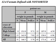
12.4 Controlling Order Using the NOTSORTED Option

Normally when a user-defined format is created, the format is internally placed into sorted order. Consequently it does not particularly matter what order the value/label pairings are specified in the value statement. However, this reordering can be prevented by using the NOTSORTED option on the VALUE statement . When applied, the internal order of the format remains as it is defined. When an ORDER=FORMATTED option is applied to a format that is created using the NOTSORTED option, the order of the pairings in the format definition is used.

In the PROC TABULATE example in Section 12.3 ‘College’ appears first because it is first alphabetically. Here the format is created using the NOTSORTED option. Since the level for ‘High School’ is listed first in the following PROC FORMAT, ‘High School’ will appear before ‘College’ in the report.

proc format;

   value edlevel (notsorted)

      9-12 = 'High School'

      13-high='College';

   run;

proc tabulate data=advrpt.demog;

   class edu sex;

   var wt;

   table edu all,

         sex*wt*(n*f=2. mean*f=5.1 stderr*f=6.2);

   format edu edlevel.;

   run;

When the NOTSORTED option is used on the VALUE statement, the order that the item pairs are defined in the VALUE statement is preserved.

The format is used as usual.

image shown here

CAVEAT

When a format is created it is optimized internally to make the assignment process as efficient as possible. Using the NOTSORTED option negates some of that optimization; however, for formats with fewer than a dozen or so value pairs it generally makes little practical difference. For very large formats (hundreds or thousands of items) there may be some performance access issues when using the NOTSORTED option. Be sure to experiment with your data and OS when using this option for larger formats.

12.5 Extending the Use of Format Translations

A user-defined format can be used to point to another secondary format or, in SAS 9.3, even a function. This allows us to create customized formats that retain characteristics of either another format or a function. The format or function call appears unquoted on the right side of the equal sign (in the label area) in square brackets.

12.5.1 Filtering Missing Values

We need to create a format that will handle missing date values differently than non-missing values. In the MISSDATE. format to the left, missing values are mapped to the word ‘Unknown’ , while all other values are formatted using the DATE9. format.

proc format;

   value missdate

      . = 'Unknown'

      other=[date9.];

   run;

proc print data=advrpt.demog;

   var lname fname dob;

   format dob missdate.;

   run;

The label for the ‘other’ category is the secondary or nested format. It is enclosed in square brackets instead of quotes.

The nested format is used as is any other format.

12.5 Nested Formats

Obs    lname        fname        dob

  1    Adams        Mary      12AUG1951

  2    Adamson      Joan      Unknown

  3    Alexander    Mark      15JAN1930

  4    Antler       Peter     15JAN1934

. . . . portions of the listing not shown . . . .

The first few lines of the listing generated by PROC PRINT show that the date of birth has been formatted. Since Joan Adamson’s date of birth is missing, it has been displayed as ‘Unknown’.

Similar nested formats can be used to check for valid data or data that can be formatted. This is the case with the PCTZERO. format which is used to map missing values to special characters for reporting purposes. Here missing values are mapped to ‘0.00’, while the non-missing values are displayed using the 6.2 format.

proc format;

   value pctzero

      .='0.00'

      other=[6.2];

   run;

12.5.2 Mapping Overlapping Ranges

Another use of nested formats is to define ranges or groups with multiple ranges. Notice here that the ‘Secondary’ and ‘Out of Range’ groups span the ‘Primary’ group. A change to one group definition requires a change to another’s as well.

proc format;

   value agegrps

      low - 40  = 'Out of Range'

      40 - <48  = 'Secondary'

      48 -  52  = 'Primary'

      52<-  65  = 'Secondary'

      65<- high = 'Out of Range'

      other = 'Unknown';

   run;

Instead we can create a series of nested formats that call each other. Although potentially more work to set up initially, these formats offer more flexibility because the range for each group is totally self-contained. The format for the inner most range (PRIMARY.) is called first, and if the value is outside of the primary range, the secondary range format (SECOND.) is called. Notice that the secondary range spans the primary range. In automated systems this can be a huge advantage.

proc format;

   value primary

      48 -  52  = 'Primary'

      other = [second.];

   value second

      40 - 65   = 'Secondary'

      other = [OOR.];

   value oor

      low - high = 'Out of Range'

      other = 'Unknown';

   run;

agegroup = put(startage,primary.);

In an assignment statement the format is used as any other format might be used:

12.5.3 Handling Text within Numeric Values

SAS supports up to 28 types of numeric missing values (see Section 2.10.1). These sometimes need to be associated with codes in the data. When importing data from raw text files, the codes themselves may be inserted as non-numeric values into the numeric fields. We need the ability to read the column as a numeric value while differentiating among the various codes.

The informat INAGE. converts selected codes into the specific missing values .S and .Y. All other non-numeric codes will map to the standard numeric missing (.). The data set SURVEYAGE contains the following values. Remember that special numeric missing values print without the period.

proc format;

  invalue inage

    y, yz = .y

    s, ss = .s

    other = [2.];

  run;

data surveyAge;

  input patcode $

        age inage.;

  datalines;

1 45

2 yz

3 36

4 ss

5 y

  run;

Obs    patcode    age

 1        1        45

 2        2         Y

 3        3        36

 4        4         S

 5        5         Y

MORE INFORMATION

The use of special numeric missing values is discussed in Section 2.10.1. A numeric informat similar to this one is created from a data set in Section 6.7.3.

12.5.4 Using Perl Regular Expressions within Format Definitions

Starting in SAS 9.3 the REGEXPE option can appear on the value side of the equal sign for a value/label pair. This option follows a quoted Perl regular expression and causes the format to effectively act like the PRXCHANGE function.

The $ABC2DEF. informat shown here has been created to convert the letter combination ‘abc’ to ‘def’.

proc format;

   invalue $abc2def (default=20)

      's/abc/def/' (REGEXPE)  = _same_;

   run;

data _null_;

x=input('abc',$abc2def.);   put x=;

x=input('xabcx',$abc2def.); put x=;

x=input('xyz',$abc2def.);   put x=;

x=input('def',$abc2def.);   put x=;

run;

The informat $ABC2DEF. is defined with a default length of 20.

The PRX string is defined and followed by the REGEXPE option, which causes the PRX string to be interpreted as a Perl Regular eXpression.

The special _SAME_ operator is used to pass the result of the PRX string to the format’s label.

The LOG shows that both a stand-alone occurrence and an embedded occurrence of ‘abc’ are converted to ‘def’.

Letter combinations other than ‘abc’ are not changed and are therefore passed through the format ‘as-is’.

x=def

x=xdefx

x=xyz

x=def

12.5.5 Passing Values to a Function as a Format Label

Starting with SAS 9.3 it is possible to pass values into functions via formats. The huge advantage is that the functions, which are embedded into the format, become available outside the DATA step, and can be used wherever formats are used.

proc format;

  value fmtname (default=10)

        other=[myfunc()];

run;

The function call occurs in the label portion of the value/label pair and is enclosed in square brackets. The specifications include:

The function may take no more than one argument.
Numeric functions return numeric values.
Character functions return character values.
The DEFAULT= option should be used to ensure proper widths.
The function can be supplied by SAS or it can be user supplied through the use of PROC FCMP (see Section 15.2).

Using SAS Supplied Functions

The FIPSTATE function can be used to convert a FIPS state code into a two-letter state postal code abbreviation; however, there is no matching format to perform the same conversion. Here we use a format to pass the FIPS code to the FIPSTATE function. As is shown in the LOG, the FIPSTATE. format returns the 2-character abbreviation.

proc format;

  value fipstate

     other=[fipstate()];

  run;

data _null_;

     x=37; put x=fipstate.;

     run;

x=NC

The use of functions in formats opens a wide range of possibilities including the use of DATE, DATETIME, and TIME functions. In this example both numeric and character versions of a series of formats are created that execute various functions. Notice that conversion between numeric and character values will occur as needed.

proc format;

  value daten   (default=10) other=[date()];

  value $datec  (default=10) other=[date()];

  value dpartn  (default=10) other=[datepart()];

  value $dpartc (default=10) other=[datepart()];

  value lenn    (default=10) other=[length()];

  value $lenc   (default=10) other=[length()];

  run;

data _null_;

  x=datetime();

  y=put(datetime(),best12.);

  z=put(date(),best12.);

  a=datepart(x);

  put x= y= z= a=;

  put x=daten.  x=dpartn.  x=lenn.;

  put y=$datec. y=$dpartc. y=$lenc.;

  put z=$datec. z=$dpartc. z=$lenc.;

  run;

The DATE function does not take an argument, but it can still be used within a format label.

The DATEPART function will extract the date portion from a datetime value.

The LENGTH function will provide the length of the argument. Although, the LENGTH function expects a character argument, a numeric value will be converted to a character value which will subsequently be passed to the LENGTH function.

A DATA _NULL_ step is used to create some numeric and character date and datetime values which are then used with the formats that were just created.

X is a numeric value containing the current datetime value in seconds (there are 10 digits in the number of seconds). The execution shown here took place on day 18,946 (15nov2011).

Y is a character variable of length 12 containing the number of seconds for the current datetime value.

Z is a character variable of length 12 with the current date.

A is the numeric date portion of the datetime value stored in X.

The DATEN. and $DATEC. formats correctly return the current date value.

The DPARTN. and DPARTC. formats return the date portion of the datetime value in days. The variable Z already contains a date value. The $DPARTC. format interprets this value as seconds and returns the date value of 0 (01jan1960). This shows that although the value is character it can be handled by the function as numeric.

x=1636995477.6 y=1636995477.6 z=18946 a=18946

x=18946 x=18946 x=10

y=18946 y=18946 y=12

z=18946 z=0     z=12

The LENGTH function is applied to the incoming value. Notice that for the variable X the numeric format (LENN.) is applied and only the number of whole numbers is counted (10). The character format ($LENC.) returns 12 when applied to the same number.

Using User-Defined Functions

When combined with user-defined functions, the ability to insert a value into a function through a format can be especially powerful.

In this example the user-defined functions C2FF() and F2CC() are used to convert between degrees Centigrade and degrees Fahrenheit. These two character functions add the scale symbols to the resultant value. Similar numeric functions that do not add the scale symbols are created in Section 15.2.2.

proc fcmp

      outlib=Advrpt.functions.Conversions;

   function c2ff(c) $;

      return(cats(((9*c)/5)+32,'°F'));

   endsub;

   function f2cc(f) $;

      return(cats((f-32)*5/9,'°C'));

   endsub;

   run;

options cmplib=(advrpt.functions);

data _null_;

     f=c2ff(100); put f=;

     c=f2cc(212); put c=;

     run;

The OUTLIB= option specifies the data set and packet (CONVERSIONS) that will contain this function definition.

The FUNCTION statement names the new function and its arguments. The $ is used to specify that this function returns a character value.

The RETURN statement contains the value to be returned by the function. In this case the result of the conversion equation is concatenated to the temperature scale symbol.

FUNCTION definitions are terminated with the ENDSUB statement.

The CMPLIB option is used to point to the data set (ADVRPT.FUNCTIONS) that contains the function definition.

A constant value (100°C ) is converted using the C2FF() function, and the converted value is displayed using a PUT statement.

f=212°F

c=100°C

These two functions can be used wherever functions can be used; however, since most procedures will not accept the use of functions, they are not as generally usable as formats. Below these two functions are called by formats so that they can be used wherever formats can be used. This includes in the PUT statement where formats are anticipated and functions are not callable.

Since the C2FF() and F2CC() functions do not have more than one argument, they can be used directly in the label portion of a user-defined format. Although in this example the format name and the function name are the same, this is not in any way a requirement.

proc format;

  value c2ff (default=10)

    other=[c2ff()];

  value f2cc (default=10)

    other=[f2cc()];

     run;

data _null_;

     c=100; put c=c2ff.;

     f=212; put f=f2cc.;

     run;

When using a function in the label it is best to set the default display width.

The function is called from within the label by enclosing it in square brackets.

The format is requested on the PUT statement. This request results in the execution of the function, and generates this text in the LOG.

c=212°F

f=100°C

The initial versions of these functions were written by Rick Langston, senior manager in software development at SAS.

Return the Quarter without the Year (Qq instead of yyQq)

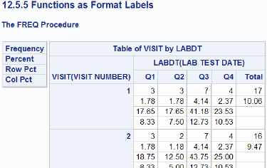
In Section 15.2.1 the QNUM() function is created to remove the year portion of the value that is returned by the YYQ. format. In that example a second DATA step was required before we could use the results of the function in a PROC FREQ step. By using that function in a format, we can use the format directly in the PROC step and thereby avoid an additional pass of the data.

Here the QNUM() function is used in the format label. The format is then used in the PROC FREQ step. The elimination of steps will almost always improve processing efficiency.

proc format;

   value qfmt other=[qnum()];

run;

options cmplib=(advrpt.functions);

proc freq data=advrpt.lab_chemistry

          order=formatted;

   table visit*labdt;

   format labdt qfmt.;

   run;

image shown here

Informats can also be used with functions-as-labels. This is a case where the user wanted the feature of the TRAILSGN informat, but that informat does not handle implied decimal specifications. In this example the numbers in the data have been entered without the decimal point (the value 12 should be .12). The function will use the TRAILSGN informat and then divide by 100 and return the result.

proc fcmp outlib=work.functions.smd;

   function tsgn(text $);

      put 'in tsgn: ' text=;

      x = input(text,trailsgn10.);

      x = x/100;

      return(x);

   endsub;

run;

options cmplib=(work.functions);

proc format;

  invalue tsgn(default=10)

    other=[tsgn()];

data _null_;

   input x: tsgn.;

   put x=;

cards;

1-

12-

123-

123+

1+

run;

1    x=.01

1-   x=-0.01

12-  x=-0.12

123- x=-1.23

123+ x=1.23

1+   x=0.01

0    x=0

MORE INFORMATION

Details on the use of PROC FCMP to create user-defined functions can be found in Section 15.2.

12.6 ANYDATE Informats

The ANYDATE informats (available starting in SAS 9) are designed to allow you to read in a variety of mixed date forms including:

DATE, DATETIME, and TIME
DDMMYY, MMDDYY, and YYMMDD
JULIAN, MONYY, and YYQ.

There are various forms of these informats:

ANYDTDTE.	extracts the date portion
ANYDTDTM.	extracts the datetime portion
ANYDTTME.	extracts the time portion

12.6.1 Reading in Mixed Dates

This example demonstrates the flexibility of these informats. Here the ANYDTDTE10. informat is applied to a number of different date forms. The DATESTYLE system option is used to resolve some of the possible ambiguities by declaring a default ordering for the month/day/year portions of the dates.

12.6 ANYDATE Informats

Obs         date

 1     13JAN2003

 2     13JAN2003

 3     13JAN2003

 4     13JAN2003

 5     03JAN2013

 6     02JAN2003

 7     02MAR2001

options datestyle=mdy;

data new;

input date anydtdte10.;

format date date9.;

datalines;

01/13/2003

13/01/2003

13jan2003

13jan03

13/01/03

01/02/03

03/02/01

run;

A PROC PRINT of the data set shows that these date values have been read into the data set as SAS dates. The supported date forms are quite varied and include DATE9. . You should note that the DATESTYLE= option cannot fully resolve all ambiguities and, consequently, some dates may be misinterpreted. Since 13 is not a valid number for a month , the informat assumes that the order of the values has been changed and it guesses that the correct order is YMD. Since the informats can detect invalid values and make informed guesses as to the correct order of the date portions, it becomes very important for the user to either know the data well, or to at the very least, understand exactly how the incoming values can be converted. In this example it is likely that should have been read as dd/mm/yy and not yy/mm/dd.

12.6.2 Converting Mixed DATETIME Values

When the incoming string contains not only dates, but time values as well, the conversion process becomes even more complicated. For the time portion (and the following applies to SAS time values as well), the hours can be specified using the 24 hour clock or the 12 hour clock with AM/PM also included.

Datetime strings might include values such as those shown to the right. With the exception of the ambiguous date with a two-digit year the ANYDTDTM informat will correctly interpret the date time portion of these strings. It is unable, however, to utilize the AM/PM codes, which are ignored.

10/13/2011:15:45:12

2011-03-01T15:20:45

9/13/2011 11:52:54 AM

9/13/2011 11:52:54 PM

13/09/2011 11:52:54 PM

11/09/12 11:52:54 AM

2011/09/12 11:52:54 PM

Fortunately the MDYAMPM. informat is available. This informat correctly interprets the AM/PM portion of the datetime value; however, it requires that the date portion be in MDY order.

Since there is no informat that will effectively combine the flexibility of the ANYDTDTM. informat with the ability to interpret the AM/PM, the following adjustment can be used. The ANYDTDTM. informat is used to convert the datetime string. The INPUT function returns the datetime value in seconds. If a ‘PM’ is present we need to add 12 hours worth of seconds (43,200=12*60*60) to the datetime value. The INDEX function searches for an occurrence of ‘PM’ and the location is converted to a binary 0/1 value which is multiplied by the number of seconds to add.

12.7 Building Formats from Data Sets

The VALUE, INVALUE, and PICTURE statements are usually used to create a user-defined format or informat. As the number of value pairs becomes large, coding these statements becomes inconvenient (for me large can be less than a dozen). Fortunately you can also define formats and informats using a data set.

PROC FORMAT accepts a data set to control the definition of the format or informat. The procedure expects specific variables, and the observations of the data set are used to form the value pairs. As a minimum the data set used to control the formation of the format must contain the variables FMTNAME, START, and LABEL . It may also contain over twenty other variables that can be used to define the format.

In this example the data set CNTRLFMT will be used create a character format ($CL_REG.) that will map the clinic number (CLINNUM) into a region (REGION).

data cntrlfmt(keep=fmtname start label);

   set advrpt.clinicnames(rename=( clinnum=start

                                   region=label));

   retain fmtname '$cl_reg';

   run;

proc format cntlin=cntrlfmt;

   run;

You may keep variables that will not be used by PROC FORMAT. Extraneous variables will be ignored.

The variable START contains the data value that is to be mapped (left side of the value pair), while LABEL is the value that will appear as a result of the mapping.

The character variable FMTNAME contains the name of the format that is to be created.

The CNTLIN= option is used to specify the data set that contains the format definition.

The control data set may define more than one format definition; however, if it does the data set must be sorted by format name (or at least grouped by format name). In the following example each incoming observation is used to build two formats ($CL_REG. and $CL_NAME.). Notice that the control data set has been sorted by the format name prior to passing it to the FORMAT procedure.

data cntrlfmt(keep=fmtname start label);

   set advrpt.clinicnames(rename=( clinnum=start));

   length fmtname $8 label $40;

   fmtname = '$cl_reg';

   label = region;

   output cntrlfmt;

   fmtname = '$cl_name';

   label = clinname;

   output cntrlfmt;

   run;

proc sort data=cntrlfmt;

   by fmtname start;

   run;

proc format cntlin=cntrlfmt;

   run;

The list of potential variables in the control data set that can be utilized by PROC FORMAT is quite extensive, and while they are well documented, you can use PROC FORMAT and the CNTLOUT= option to surface the format definition by writing it to a data set. This will reveal the variable names that can be used in a format definition and can give you a good idea about their usage.

proc format cntlout=control(where=(fmtname='CL_NAME'));

   run;

proc print data=control;

   run;

12.7 Building Formats from Data

D L

      F                                                    D                        D A A

      M                                                    E  L   P     N         D I T N

      T      S           L                                 F  E   R     O   S E   E G A G

      N      T           A                                 A  N F E M F E T E E   C 3 T U

 O    A      A      E    B                           M  M  U  G U F U I D Y X X H S S Y A

 b    M      R      N    E                           I  A  L  T Z I L L I P C C L E E P G

 s    E      T      D    L                           N  X  T  H Z X T L T E L L O P P E E

 1 CL_NAME 011234 011234 Boston National Medical     1 40 27 27 0   0   0 C N N

 2 CL_NAME 014321 014321 Vermont Treatment Center    1 40 27 27 0   0   0 C N N

 3 CL_NAME 023910 023910 New York Metro Medical Ctr  1 40 27 27 0   0   0 C N N

 4 CL_NAME 024477 024477 New York General Hospital   1 40 27 27 0   0   0 C N N

 5 CL_NAME 026789 026789 Geneva Memorial Hospital    1 40 27 27 0   0   0 C N N

data intervals(keep=fmtname start end label hlo);

  retain fmtname 'studydt';

  length label $20;

  start = '12jan2006:01:01:01'dt;

  end = '24nov2007:11:12:13'dt;

  label = 'datetime18.';

  hlo = 'F';

  output intervals;

  start=.;

  end=.;

  hlo='O';

  label= 'Out of Compliance' ;

  output intervals;

  run;

proc format cntlin=intervals;

  run;

The HLO variable can be especially useful because it allows you to specify not only the HIGH and LOW open ended ranges, but the keyword OTHER as well. Another less known usage of HLO is to specify a nested format (HLO=’F’) . The format STUDYDT., created here, sets the acceptable range of dates for the study. All other dates will be displayed as ‘Out of Compliance’.

Although set to missing in this example, the START and END variables do not need to be cleared for the observation containing HLO=’O’.

MORE INFORMATION

An example in Section 6.5 creates a format from data in order to perform a table lookup. The example in Section 12.3.2 creates a multilabel format based on data generated in a DATA step.

12.8 Using the PVALUE Format

When displaying values between zero and one, especially values close to zero, it is often difficult to determine the number of decimal values needed. The PVALUE. format was designed to display small probability values. The number of decimal points (4 in this table) designates the smallest number that can be displayed by the format. Smaller numbers will be displayed with a < sign.

X	PVALUE6.4 `➊`
`0.000000`	`<.0001`
`0.000006`	`<.0001`
`0.000050`	`<.0001`
`0.000100`	`<.0001`
`0.000400`	`0.0004`
`0.003000`	`0.0030`
`0.020000`	`0.0200`
`0.100000`	`0.1000`

This format was designed to work with probability values that are necessarily constrained to be between 0 and 1, consequently this format does not handle negative values or even 0 well. All values less than the minimum specified (for PVALUE6.4 this is .0001) will be displayed the same (as <.0001). Even the minimum (.0001) is displayed as <.0001.

If you want to take advantage of the capabilities of the PVALUE format, but suspect that some numbers will be equal to or less than zero or even greater than one, then you may want to create a format that incorporates, but does not solely depend on PVALUE.

Here the RANGE. format is created using a combination of formats.

proc format;

 value range

  low - <0 = [best7.]

  0        = [1.]

  0<  -  1 = [pvalue6.4]

  1<  -high= [best6.];

 run;

The table below shows how various values (I) are displayed using the PVALUE7.4 format (J) and the RANGE. format (K).

12.8 Using the PVALUE Format

Obs           i          j       k

  1        -4.1     <.0001       -4.1

  2     -0.0001     <.0001    -0.0001

  3    -0.00001     <.0001      -1E-5

  4           0     <.0001    0

  5     0.00001     <.0001    <.0001

  6     0.00001     <.0001    <.0001

  7      0.0003     0.0003    0.0003

  8        0.02     0.0200    0.0200

  9         0.1     0.1000    0.1000

 10           1     1.0000    1.0000

 11       12.34    12.3400     12.34

 12    3456.789    3456.79    3456.8

12.9 Format Libraries

User-defined formats and informats are saved in a catalog, which by default will have the name FORMATS. When a format library is not named on the PROC FORMAT statement, the format definition is written to the catalog WORK.FORMATS. The entry name is the same as the format. Here the definition of the TONS. format will be stored in WORK.FORMATS.TONS.FORMAT.

proc format;

  picture Tons

     0 =  '9'

.... code not shown ....

The catalog entry type will depend on the type of format that is created:

FORMAT	Numeric format
FORMATC	Character format
INFMT	Numeric informat
INFMTC	Character informat

Because each of the four types has a different catalog entry type, the same format name can be used up to four times.

12.9.1 Saving Formats Permanently

Formats are stored permanently by using the LIBRARY= option on the PROC FORMAT statement. The LIBRARY= option is used to specify the libref that is to contain the FORMATS catalog. Any formats created by this PROC FORMAT will be stored in a catalog with the name of FORMATS in the libref ADVRPT.

proc format library=advrpt;

.... code not shown ....

Because of the way that SAS searches for format catalogs (see Section 12.9.2), formats that are stored in a catalog named FORMATS in a libref named LIBRARY will by default be included in the search path. The code at first seems a bit odd, but this FORMAT step will create or add to the catalog LIBRARY.FORMATS.

libname library 'c:myfmts';

proc format library=library;

.... code not shown ....

Although I find it to be generally a good idea, you are not required to store the format definitions in a catalog named FORMATS. You can specify the catalog name as a second level on the LIBRARY= option. Here the catalog will be named PROJFMT.

proc format library=advrpt.projfmt;

.... code not shown ....

12.9.2 Searching for Formats

When requesting a format SAS first checks in WORK.FORMATS and then, if the libref LIBRARY is defined, SAS will look in LIBRARY.FORMATS. Since format libraries are not usually conveniently located in these two locations, we need to be able to search for formats in a variety of places and in catalogs named something other than FORMATS.

The FMTSEARCH= system option is used to identify not only the librefs, but also the order for the search. In this example SAS will look for the requested format in the catalog ADVRPT.PROJFMT, and then in catalogs named FORMATS in the librefs WORK and LIBRARY in that order. Since WORK appears in the FMTSEARCH list, the default catalog is no longer WORK.FORMATS, and it is not searched first.

options fmtsearch=(advrpt.projfmt work library);

12.9.3 Concatenating Format Catalogs and Libraries

When your formats are spread among multiple catalogs, the search can be simplified by concatenating the catalogs.

Catalogs with the same name will be implicitly concatenated when they reside within concatenated libraries. In the following example formats are being written to two different libraries (the librefs are OLDFMT and NEWFMT).

libname oldfmt 'c:	emp1';

libname newfmt 'c:	emp2';

libname allfmt (newfmt oldfmt);

proc format library=oldfmt;

  value yesno 1 = 'Yes'

              0 = 'No';

  value generation

   low - <1950 = 'Greatest'

   1950 - high = 'Boomer';

  run;

proc format library=newfmt;

  value gender 1 = 'Female'

               0 = 'Male';

  value yesno 1 = 'No'

              0 = 'Yes';

  run;

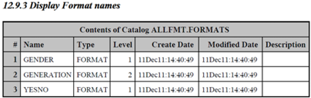
title1 12.9.3 Display Format names;

proc catalog cat=allfmt.formats;

  contents;

  quit;

options fmtsearch=(allfmt work);

Any references to the libref ALLFMT will point to both of the other two locations.

The YESNO. format appears in both format libraries. Notice that the two definitions are not the same.

PROC CATALOG is used here to show the locations of the formats. The column LEVEL refers to the library containing the catalog that contains the format.

Before any of the formats in the ALLFMT library can be used, the library must be included on the search path. Formats in ALLFMT will be found before any formats with the same name in the WORK library. Within ALLFMT the catalogs are searched from left to right. The version of the YESNO. format in the NEWFMT library will be used.

The output generated by the CATALOG procedure shows that the various formats can be found in the concatenated library ALLFMT. It also shows that the YESNO. format, which is defined in both the OLDFMT and NEWFMT catalogs is being picked up from the first catalog in the list (NEWFMT – LEVEL=1).

image shown here

..................Content has been hidden....................

You can't read the all page of ebook, please click here login for view all page.

Table of Contents for Chapter 12 Taking Advantage of Formats

Create new playlist

Sign In

Sign Up

Chapter 12 Taking Advantage of Formats

MORE INFORMATION

SEE ALSO

12.1 Using Preloaded Formats to Modify Report Contents

12.1.1 Using Preloaded Formats with PROC REPORT

Using PRELOADFMT with EXCLUSIVE

Using COMPLETEROWS without EXCLUSIVE

Using COMPLETEROWS with EXCLUSIVE

12.1.2 Using Preloaded Formats with PROC TABULATE

PRELOADFMT with EXCLUSIVE

Using PRELOADFMT without EXCLUSIVE

MORE INFORMATION

SEE ALSO

12.1.3 Using Preloaded Formats with the MEANS and SUMMARY Procedures

Using PRELOADFMT with EXCLUSIVE

Using COMPLETETYPES with PRELOADFMT and EXCLUSIVE

Using COMPLETETYPES without EXCLUSIVE

12.2 Doing More with Picture Formats

SEE ALSO

12.2.1 Date Directives and the DATATYPE Option

SAS 9.3 Date Directive Enhancements

12.2.2 Working with Fractional Values

12.2.3 Using the MULT and PREFIX Options

SEE ALSO

12.2.4 Display Granularity Based on Value Ranges – Limiting Significant Digits

12.3 Multilabel (MLF) Formats

12.3.1 A Simple MLF

MORE INFORMATION

12.3.2 Calculating Rolling Averages

MORE INFORMATION

SEE ALSO

12.4 Controlling Order Using the NOTSORTED Option

CAVEAT

12.5 Extending the Use of Format Translations

12.5.1 Filtering Missing Values

12.5.2 Mapping Overlapping Ranges

12.5.3 Handling Text within Numeric Values

MORE INFORMATION

SEE ALSO

12.5.4 Using Perl Regular Expressions within Format Definitions

12.5.5 Passing Values to a Function as a Format Label

Using SAS Supplied Functions

Using User-Defined Functions

Return the Quarter without the Year (Qq instead of yyQq)

MORE INFORMATION

12.6 ANYDATE Informats

12.6.1 Reading in Mixed Dates

12.6.2 Converting Mixed DATETIME Values

12.7 Building Formats from Data Sets

MORE INFORMATION

SEE ALSO

12.8 Using the PVALUE Format

12.9 Format Libraries

12.9.1 Saving Formats Permanently

12.9.2 Searching for Formats

12.9.3 Concatenating Format Catalogs and Libraries

Table of Contents for
Chapter 12 Taking Advantage of Formats

Chapter `12` Taking Advantage of Formats