
A multinomial distribution is one where every observation in the dataset is taken from one of a limited number of options. For example, in the race census data, race is a multinomial parameter: it can be one of seven options. If the census were a sample, how good of an estimate of the population would the ratios of the race observations be?
Bayesian methods work by updating a prior probability distribution on the data with more data. For multivariate data, the Dirichlet distribution is commonly used. The Bayesian process observes how many times each option is seen and returns an estimate of the ratios of the different options from the multimodal distribution.
So in the case of the census race data, this algorithm looks at the ratios from a sample and updates the prior distribution from those values. The output is a belief about the probabilities of those ratios in the population.
We'll need these dependencies:
(defproject statim "0.1.0"
  :dependencies [[org.clojure/clojure "1.6.0"]
                 [incanter "1.5.5"]])
We'll also use these requirements:
(require
  '[incanter.core :as i]
  'incanter.io
  '[incanter.bayes :as b]
  '[incanter.stats :as s])
For data, we'll use the census race table for Virginia, just as we did in the Differencing Variables to Show Changes recipe.
For this recipe, we'll first load the data, perform the Bayesian analysis, and finally summarize the values from the distribution returned. We'll get the median, standard deviation, and confidence interval:
- First, we need to load the data. When we do, we'll rename the fields to make them easier to work with. We'll also pull out a sample to work with, so we can compare our results against the population when we're done:
(def census-race (i/col-names (incanter.io/read-dataset "data/all_160_in_51.P3.csv" :header true) [:geoid :sumlev :state :county :cbsa :csa :necta :cnecta :name :pop :pop2k :housing :housing2k :total :total2k :white :white2k :black :black2k :indian :indian2k :asian :asian2k :hawaiian :hawaiian2k :other :other2k :multiple :multiple2k])) (def census-sample (s/sample census-race :size 60)) - We'll now pull out the race columns and total them:
(def race-keys [:white :black :indian :asian :hawaiian :other :multiple]) (def race-totals (into {} (map #(vector % (i/sum (i/$ % census-sample))) race-keys))) - Next, we'll pull out just the sums from the totals map:
(def y (map second (sort race-totals)))
- We will draw samples for this from the Dirichlet distribution, using
sample-multinomial-params, and put those into a new map associated with their original key:(def theta (b/sample-multinomial-params 2000 y)) (def theta-params (into {} (map #(vector %1 (i/sel theta :cols %2)) (sort race-keys) (range)))) - We can now summarize these by calling basic statistical functions on the distributions returned. In this case, we're curious about the distribution of these summary statistics in the population of which our data is a sample. For example, in this case, African-Americans are almost 24 percent:
user=> (s/mean (:black theta-params))
0.17924288261591886
user=> (s/sd (:black theta-params))
3.636147768790565E-4
user=> (s/quantile (:black theta-params)
         :probs [0.025 0.975])
(0.17853910580802798 0.17995015497863504)
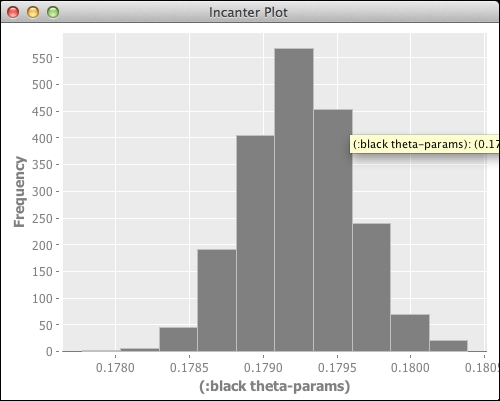
- A histogram of the proportions can also be helpful:
(i/view (c/histogram (:black theta-params)))
The real test of this system is how well it has modeled the population. We can find that out easily by dividing the total African-American population by the total population:
user=> (/ (i/sum (i/sel census-race :cols :black))
          (i/sum (i/sel census-race :cols :total)))
0.21676297226785196
user=> (- *1 (s/mean (:black theta-params)))
0.0375200896519331
So in fact, the results are close, but not very.
Let's reiterate what we we've learned about Bayesian analysis by looking at what this process has done. It started out with a standard distribution (the Dirichlet distribution), and based upon input data from the sample, updated its estimate of the probability distribution of the population that the sample was drawn from.
Often Bayesian methods provide better results than alternative methods, and they're a powerful addition to any data worker's tool set.
Incanter includes functions that sample from a number of Bayesian distributions, found at http://liebke.github.com/incanter/bayes-api.html.
On Bayesian approaches to data analysis, and life in general, see http://bayes.bgsu.edu/nsf_web/tutorial/a_brief_tutorial.htm and http://dartthrowingchimp.wordpress.com/2012/12/31/dr-bayes-or-how-i-learned-to-stop-worrying-and-love-updating/.