
CCHP Decision-Making
Abstract
Keywords
Multicriteria decision-making
fuzzy logic
grey incidence approach
climate
CCHP
4.1. Introduction
Every decision we make about the essential components of the CCHP system, including the power generation unit, the cooling system, and the heat recovery system, changes the quality and quantity of all of the criteria and subcriteria that were discussed in Chapter 3.
As discussed in Chapters 1 and 2, there are several options for each main component of the CCHP system. Available prime movers include different types of industrial gas and steam turbines, micro-gas turbines (MGTs), micro-steam turbines (MSTs), internal combustion engines (compression ignition, spark ignition), different types of external combustion Stirling engines, and fuel cells.
Each of the above technologies can be coupled with photovoltaic (PV) cells or electricity storage systems to provide or store extra electricity to fulfill the electrical demand of the building or sell it during electrical peak hours at higher prices.
The heat in the CCHP systems is recovered, generated, or stored for three purposes. Heat is used for heating spaces via terminal stations such as fan coil units on cold days, cooling spaces via absorption or adsorption chillers on hot days, and providing the domestic hot water demand of the target building during the year.
The domestic hot water system can be either integrated with or separated from the CCHP system. When it is separated from the CCHP system, the hot water can be provided by using a solar water heater or a gas fired water heater. When it is integrated with the CCHP system, it uses the recoverable heat from the prime mover, auxiliary heating system, or solar water heater.
Calculations must be done to compare the technological, economic, etc. characteristics of the CCHP system to decide whether the domestic hot water should be integrated with or separated from the CCHP system.
Addition of any new component such as an electrical compression chiller, solar PV cells, electricity storage system, solar water heater, auxiliary heating system, or heat storage system to the basic CCHP unit changes the CCHP’s characteristics. Comprehensive evaluations must be done prior to decision-making and the addition of any new component.
According to the discussion presented above, decision-making can be divided into two levels:
1. Basic decision-making
2. Design decision-making
In the basic decision-making process (which is the main concern of this chapter), only the basic components (the prime mover, cooling system, and heating system) are decided (Figure 4.1). For this purpose multicriteria decision-making (MCDM) methods will be introduced.

However, in the design decision-making process (which is a part of detail design and will be presented in the following chapters), decisions are made about the presence, position and size of the components in the CCHP cycle, (Figure 4.2).

Different and numerous criteria are encountered during the decision-making process for the basic components of a CCHP system. The most important criteria involved in the decision-making process are presented in the previous chapter. They have the following characteristics:
• Some of the criteria are qualitative (maturity, UFCR, OPL, LAEM).
• The criteria have different dimensions (NPV ($), noise (db), PB (year)).
• The criteria have different orders of magnitude (0 < FESR <1, NPV can be as high as 105).
• The criteria have different levels of importance (FESR is more important than OPL or PHR, …).
• There are numerous important criteria (FESR, NPV, IRR, IEL, …).
Decision-making based on the above criteria with all their different characteristics is very difficult. MCDM must be able to compromise between all different criteria, and for this purpose it must have the following abilities:
1. It must make all of the qualitative criteria quantitative.
2. It must present all the criteria in dimensionless form.
3. It must normalize all the criteria (they all should be in the same range)
4. It must give normalized weight to each criterion and subcriterion according to the available technical data and knowledge of the decision-maker.
5. It must integrate all of the criteria into one or a limited number of criteria to make the decision-making easier.
4.2. Multicriteria Decision-Making (MCDM)
Probability and statistics, fuzzy mathematics, and grey systems theory are the three most commonly used research methods employed for the investigation of uncertain systems [1]. Decision-making for CCHP components includes uncertain parameters such as maturity, PHR, OPL, LAEM, IEL, UFCR, etc. They are uncertain parameters because they are judged with linguistic concepts such as very bad, bad, moderate, good, and very good, or very low, low, medium, high, and very high. Uncertainty in these cases means that we cannot define a clear border between two neighboring qualities such as bad and very bad.
Probability and statistics studies the chance of a phenomena with an uncertain nature happening in the future based on a large statistical sample data from the past. Probability calculations start with large sample data to generate a typical statistical distribution such as normal, uniform, etc.
Zadeh (1965) [2] was the first to propose the fuzzy set. The fuzzy set includes elements with only a partial degree of membership. In recent years, the applications of fuzzy logic have increased significantly. The applications range from products such as cameras, washing machines, and microwave ovens to industrial process control and decision-making systems. Fuzzy logic starts with the concept of a fuzzy set. A fuzzy set is a set without a crisp, clearly defined boundary. It can contain elements with only a partial degree of membership. In the following three different membership functions, namely the triangular-shaped, generalized bell-shaped, and symmetric Gaussian functions, are presented. The triangular-shaped membership function can be written as [3]
fx(x, a, b, c)=max(min(x−ab−a,c−xc−b), 0)
 (4-1)
(4-1)while the generalized bell-shaped membership function can be written as
fx(x, a, b, c)=(1+|x−ca|2b)−1
 (4-2)
(4-2)In the preceding functions (a, b, c) is a triangular fuzzy number.
Finally, the symmetric Gaussian membership function, which depends on two parameters (σ, c) can be written as follows:
fx(x, σ, c)=e−(x−c)22σ2
 (4-3)
(4-3)The behavior of the preceding membership functions is depicted in Figure 4.3.

If I=(aI,bI,cI)![]() and II=(aII,bII,cII)
and II=(aII,bII,cII)![]() are two triangular fuzzy numbers, their summation, multiplication, and division are as follows:
are two triangular fuzzy numbers, their summation, multiplication, and division are as follows:
I+II=(aI+aII,bI+bII, cI+cII)I×II=(aI×aII,bI×bII, cI×cII)I/II=(aI/cII,bI/bII, cI/aII)
 (4-4)
(4-4)Grey systems theory was introduced by Deng Ju-long (1982) in China. The main capability of grey systems theory is the ability to study uncertainty problems with very few points of sample data and/or poor information; these problems are difficult with probability and the fuzzy algorithm. The grey incidence approach (GIA) is one of the main results of grey systems theory. The main idea of the GIA is that the closeness of a relationship is judged based on the degree of similarity of the geometrical patterns of sequence curves [1]. The more similar the curves are, the higher grey incidence grad (GIG) and as a result the better decision to make, and vice versa.
In the following, the two most practical techniques of the fuzzy algorithm and GIA will be introduced and applied to a similar case study to compare their results.
4.2.1. Fuzzy-MCDM Modeling
The fuzzy-MCDM method integrates numerous and different criteria to make the decision more comprehensive. In this section, the corresponding steps of the fuzzy-MCDM method are presented sequentially.
4.2.1.1. Quantifying the Qualitative Criteria
In decision-making problems, some of the criteria such as OPL, maturity, UFCR, IEL, and LAEM are qualitative and it is not easy to quantify them. The importance of a qualitative criterion depends on the technical data, and the opinion and knowledge of the decision-maker. Therefore, fuzzy-MCDM must propose a method to quantify qualities such as “very bad,” “bad,” “middle,” “good,” and “very good.” In the fuzzy-MCDM, a linguistic judgment is used and the corresponding triangular fuzzy numbers proposed by [4] are used to quantify the qualitative criteria. The linguistic judgments and their corresponding fuzzy numbers are presented in Table 4.1 [5, 6].
Table 4.1
Linguistic Judgments and Their Corresponding Fuzzy Numbers
| Linguistic Judgment | Fuzzy Judgment |
| Very low (VL) | (0, 0, 0.3) |
| Low (L) | (0, 0.3, 0.5) |
| Middle (M) | (0.3, 0.5, 0.7) |
| High (H) | (0.5, 0.7, 1.0) |
| Very high (VH) | (0.7, 1.0, 1.0) |
In what follows the uppercase letters show the fuzzy numbers and the lowercase letters indicate the real numbers.
4.2.1.2. Generating the Judgment Matrix
Fuzzy decision-making for the basic components of a CCHP system starts by generating a judgment matrix as follows:
J=[Jij]m×n
where Jij is our judgment about the ith option based on the jth criteria, with i = 1, 2…, m and j = 1, 2…, n. In addition, m and n are the number of alternatives for each component and the number of criteria, respectively.
4.2.1.3. Normalization of the Judgment Matrix
To allow criteria to be properly evaluated while comparing options, all the criteria must fall in the same range. For this purpose, the judgment matrix is normalized.
If the criterion is “the higher the better” such as the FESR then
JNij=JijJ↑j
 (4-6)
(4-6)If the criterion is “the lower the better” such as the investment cost then
JNij=J↓jJij
 (4-7)
(4-7)where in the preceding equations
J↑j=max{Jij|i=1, 2 …, m}J↓j=min{Jij|i=1, 2 …, m}
 (4-8)
(4-8)If in the normalization process a component of the triangular fuzzy number becomes greater than 1, it will be substituted with 1. Therefore, the normalized judgment matrix (JN) would be as follows:
JN=[JNij]m×n
4.2.1.4. Calculating the Normalized Weight Matrix
In MCDM methods, the degree of importance of each criterion with respect to the other criteria is considered by calculating the weight of each criterion. For this purpose, the pairwise comparison (PC) matrix between the n criteria is made as follows:
PC=[PCij]n×n
where PCij represents the importance of the ith criterion with respect to the jth criterion. In the fuzzy-MCDM, a linguistic pairwise comparison presented by [4] is used to provide the PC matrix as in Table 4.2.
Table 4.2
Fuzzy Linguistic Pairwise Comparison and Their Corresponding Fuzzy Numbers
| Linguistic Judgment | Fuzzy-PC | Fuzzy-PC(R) |
| Just equal (JE) | (1,1,1) | (1,1,1) |
| Equally important (EI) | (1/2,1,3/2) | (2/3,1,2) |
| Weakly more important (WMI) | (1,3/2,2) | (1/2,2/3,1) |
| Strongly more important (SMI) | (3/2,2,5/2) | (2/5,1/2,2/3) |
| Very strongly more important (VSMI) | (2,5/2,3) | (1/3,2/5,1/2) |
| Absolutely more important (AMI) | (5/2,3,7/2) | (2/7,1/3,2/5) |
The equation to calculate the weight of each criterion or subcriterion in the fuzzy eigenvector of the PC matrix is
Ei=[∏nj=1PCij]1/n
 (4-11)
Finally, the normalized weight matrix for each criterion and subcriterion would be calculated as follows:
Wi=Ei∑ni=1Ei
 (4-12)
4.2.1.5. Finding the Ideal and Anti-ideal Solutions for All Criteria
The case in which all the subcriteria are the best simultaneously is the ideal solution (I↑) and the case in which all the criteria are the worst simultaneously would be the anti-ideal solution (I↓). Therefore, the best and the worst solutions would be as follows:
I↑=[I↑1, I↑2 …, I↑n]I↑j=max{JNij| i=1, 2, …, m}
 (4-13)
I↓=[I↓1, I↓2 …, I↓n]I↓j=min{JNij| i=1, 2, …, m}
 (4-14)
4.2.1.6. Finding the Weighted Distance from the Ideal and Anti-ideal Solutions
In this step, we calculate the weighted distance. The distance from the ideal and anti-ideal solutions is calculated as follows:
dij↑↓(I↑↓j,JNij)=√14((a↑↓j−aNij)2+2(b↑↓j−bNij)2+(c↑↓j−cNij)2)
 (4-15)
The weighted distance can be calculated according to the following equation:
D↑↓i=∑nj=1βjWjd↑↓ij, i=1,2,…,m
 (4-16)
where β ∈ {0, 1} is the criteria coefficient and is used for the purpose of single- or multicriteria decision-making. When a criterion is supposed to be counted in the decision-making process β = 1, otherwise β = 0.
4.2.1.7. Calculating the Closeness Number (CN)
The closeness of different options to the ideal solution is calculated according to the following equations:
ND↓=min{D↓ii=1, 2, …, m}, ND↑=max{D↓ii=1, 2, …, m}PD↓=min{D↑ii=1, 2, …, m}, PD↑=max{D↑ii=1, 2, …, m}
 (4-17)
α↑↓i=d(D↑↓i,PD↓↑)+d(D↓↑i,ND↑↓)
Based on this, the closeness number (CNi) is used in the final decision-making process and is calculated as follows:
CNi=α↓iα↓i+α↑i, i=1, 2, …,m
 (4-19)
It is obvious that 0 ≤ CNi ≤ 1, therefore as CNi approaches 1 it is getting closer to the ideal solution; on the contrary if CNi approaches zero it is getting closer to the anti-ideal solution.
4.2.2. Grey-MCDM Modeling
4.2.2.1. Quantifying the Qualitative Criteria
In order to quantify the qualitative criteria, in the GIA, a letter grade from A to E is utilized, in which A represents the very good and E represents the very bad. Moreover, the scale shown in Figure 4.4 is used to quantify these letter judgments [7-9].

4.2.2.2. Generating the Judgment Matrix
The grey-MCDM starts by writing the judgment matrix as follows:
J=⌊Jij⌋m×n
where Jij is our judgment about the ith option based on the jth criteria with i = 1, 2…, m and j = 1, 2…, n. In addition, m and n are the number of alternatives for each component and the number of criteria, respectively.
For example, if the problem is to find the best type of prime mover, and there are 5 types of prime movers and 15 subcriteria, m = 5 and n = 15. If the third type of prime mover is an MGT and the first subcriteria is the FESR, then J31 = FESRMGT.
4.2.2.3. Normalization of the Judgment Matrix
In order to normalize the judgment matrix from the previous section, if the criterion (Jij) is a profit for the project and is “the higher the better” such as the UFCR, then it is normalized as below:
JNij=Jij−J↓jJ↑j−J↓j
 (4-21)
If the Jij is a cost for the project and is “the lower the better” such as IOM, then it is normalized as follows:
JNij=J↑j−JijJ↑j−J↓j
 (4-22)
where in the above equations
J↑j=max{jij|i=1,2…,m}J↓j=min{jij|i=1,2…,m}
 (4-23)
Therefore, the normalized judgment matrix (JN) would be as follows:
JN=[JNij]m×n
4.2.2.4. Calculating the Normalized Weight Matrix
To calculate the normalized weight matrix in the GIA an equation is recommended to determine the pairwise comparison (PC) matrix as follows:
PCij=1±0.1δ, δ=0, 1, 2, …, 10
where the plus sign is for the time when the ith criteria is δ degrees more important than the jth criteria, while the minus sign is for the time when the jth criteria is δ degrees more important than the ith criteria.
According to the decision-maker’s opinion and the preceding equation, Table 4.3 is recommended for the linguistic pairwise comparison in the grey-MCDM.
Table 4.3
The Quantified Grey-MCDM Linguistic Pairwise Comparison [5]
| Linguistic Judgment | Grey-PC | Grey-PC(R) |
| Just equal (JE) (δ = 0) | 1 | 1 |
| Equally important (EI) (δ = 2) | 1.2 | 0.8 |
| Weakly more important (WMI) (δ = 4) | 1.4 | 0.6 |
| Strongly more important (SMI) (δ = 6) | 1.6 | 0.4 |
| Very strongly more important (VSMI) (δ = 8) | 1.8 | 0.2 |
| Absolutely more important (AMI) (δ = 9)* | 1.9 | 0.1 |
* If δ = 10, it means that a criterion has no importance at all with respect to the other criterion, which is not true, because all the criteria have a minimum degree of importance; therefore in this case δ = 9 is more logical.
However, the improved GIA proposed by [7] uses a combined weighting method. This method uses an objective weighting method called the entropy information method (EIM) together with a subjective weighting method called the analytic hierarchy process (AHP) to make use of the advantages of both methods. The AHP is mostly based on the knowledge and opinion of the decision-maker while the EIM is based on the technical data and judgment matrix. The combined weighting method blends these two weights together.
The subjective weighting method (AHP) is briefly presented in the following:
ρj=∑ni=1PCijρmax=max(ρ1,ρ2,…,ρn)ρmin=min(ρ1,ρ2,…,ρn)θ=ρmax/ρmin
 (4-26)
bik={1+(ρi−ρk)/ρmin,ρi≥ρk,θ≠1(1+(ρi−ρk)/ρmin)−1,ρi<ρk,θ≠10θ=1
 (4-27)
cik=logbik, i,k=1, 2, …, n
dik=1n∑nl=1(cil−ckl)
 (4-29)
b′ik=10dik
Therefore, the characteristic vector of b′ik![]() is given as follows:
is given as follows:
Ei=n√∐nk=1b′ik, i=1, 2, …, n
 (4-31)
Finally, the normalized weight matrix in the AHP method would be as follows:
W1i=Ei∑ni=1Ei0≤W1i≤1, ∑ni=1W1i=1
 (4-32)
The above equation gives the normalized weight of each criterion and subcriterion in the AHP.
To compute the combined weight in the GIA, the EIM is used as the objective weighting method. In the EIM method, the proximity degree (PD) of benefit and cost criteria is calculated as follows:
PDij=JijJ↑j, for benefits
 (4-33)
PDij=J↓jJij, for costs
 (4-34)
Then the PD should be normalized as follows:
PDNij=PDij∑mj=1PDij, ∑mj=1PDNij=1
 (4-35)
The entropy of information shows the uncertainty of the criteria and can be calculated as follows:
Si=−∑mj=1PDNij ln PDNij
 (4-36)
The entropy should be normalized with the maximum entropy. According to the previous equation the maximum entropy occurs when all the elements of PDNij![]() become equal; therefore we have
become equal; therefore we have
Smax=ln mSNi=Si/SmaxS=∑ni=1SNi
 (4-37)
Finally, the weights proposed by the EIM can be calculated:
W2i=1n−S(1−SNi)0≤W2i≤1, ∑ni=1W2i=1
 (4-38)
Up to this point, the weights of the criteria and subcriteria have been calculated using the AHP and EIM; now a linear combination is used to calculate the combined weight (WC) used in the GIA:
WCi=∑2k=1λkWik, ∑2k=1λk=1
 (4-39)
In the above equation, k = 1 and k = 2 correspond to the weights calculated by the AHP and EIM, respectively. The coefficients λ1 and λ2 are calculated as follows:
(λ1, λ2)=(s1∑2k=1sk, s2∑2k=1sk)
 (4-40)
sk=exp{−[1+μ∑ni=1∑mj=1Wki(1−JNij)1−μ]}, k=1, 2
 (4-41)
where μ is the balance coefficient and 0 < μ < 1. The impact of μ on the λ’s and on decision-making will be presented in the case studies at the end this chapter.
4.2.2.5. Finding the Ideal and Anti-ideal Solutions for All Criteria
The case in which all the criteria are the best simultaneously is the ideal solution (I↑) and the case in which all the criteria are the worst simultaneously would be the anti-ideal solution (I↓). Therefore, the best and the worst solutions for the GIA are as follows:
I↑=[I↑1, I↑2 …, I↑n]I↑j=max{JNij|i=1, 2, …, m}
 (4-42)
I↓=[I↓1, I↓2 …, I↓n]I↓j=min{JNij|i=1, 2, …, m}
 (4-43)
4.2.2.6. Finding the Weighted Distance from the Ideal and Anti-ideal Solutions
The incidence coefficient between the comparative sequence and the ideal and anti-ideal solutions is calculated as
d↑↓ij(I↑↓i, JNij)=minjmini|I↑↓i−JNij|+ξmaxjmaxi|I↑↓i−JNij||I↑↓i−JNij|+ξmaxjmaxi|I↑↓i−JNij|
 (4-44)
where the minj mini |I↑↓i−JNij|![]() and maxj maxi |I↑↓i−JNij|
and maxj maxi |I↑↓i−JNij|![]() are the global minimum and maximum of absolute distance between the normalized judgment criteria from the best and worst solutions. In addition, ξ is the distinguishing coefficient, and 0 < ξ < 1. The impact of the distinguishing coefficient on decision-making is also studied in the case studies at the end of this chapter.
are the global minimum and maximum of absolute distance between the normalized judgment criteria from the best and worst solutions. In addition, ξ is the distinguishing coefficient, and 0 < ξ < 1. The impact of the distinguishing coefficient on decision-making is also studied in the case studies at the end of this chapter.
Finally, the weighted distance can be calculated according to the following equation:
D↑↓i=∑nj=1βjWCjd↑↓ij, i=1,2,…, m
 (4-45)
where β ∈ {0, 1} is the criteria coefficient and is used for the purpose of single- or multicriteria decision-making. When a criterion is supposed to be counted in the decision-making process the β = 1, otherwise β = 0.
4.2.2.7. Calculating the GIG
The grey incidence grade is used for final decision-making in the GIA and is calculated as follows:
GIGi=11+(D↓i/D↑i)2, i=1,2,…,m
 (4-46)
It is obvious that 0 ≤ GIGi ≤ 1. Therefore as GIGi approaches 1, we are approaching the ideal solution; on the contrary if GIGi approaches zero, we are getting closer to the anti-ideal solution.
4.3. Case Studies
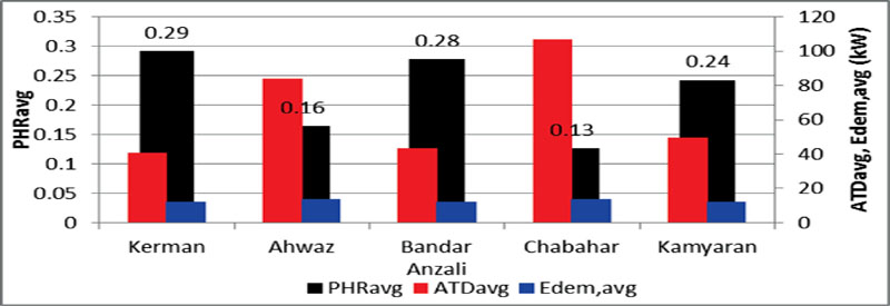
Choose the best type of prime mover for a CCHP system among the four options of conventional separate production (CSP), gas-fired internal combustion engine (IC), MGT, and Stirling engine (STR) for a four-floor, eight-unit residential building with a total living area of 1200 m2 [10]. The building is assumed to be located in one of five cities (Kerman, Ahwaz, Bandar Anzali, Chabahar, Kamyaran) with five different climates. The weather information including the maximum and minimum dry-bulb temperature (Tdb) and relative humidity (RH) of the selected cities are given in Table 4.4. In addition the annual average aggregated thermal demand (ATD), electrical demand (Edem), and power to heat ratio (PHR) of the building for the five case studies are given in Figure 4.5.
Table 4.4
Weather Information for the Representative Cities
| City | Tdb_max(oC) | Tdb_min(oC) | RHmax(%) | RHmin(%) |
| Kerman | 36.51 | −2.50 | 78 | 10 |
| Ahwaz | 46.74 | 8.73 | 86.13 | 8.76 |
| Bandar Anzali | 29.76 | 4.61 | 96.2 | 64.36 |
| Chabahar | 33.55 | 16.87 | 86.10 | 43.14 |
| Kamyaran | 36.82 | −4.88 | 85.05 | 11.38 |

4.3.1. Solution
In order to find the best type of prime mover, we apply both the fuzzy-MCDM and grey-MCDM methods to the problem, to be sure about the decision. If both methods recommend the same solution it confirms the decision. To do the calculations, MATLAB code was generated for the two MCDM methods, but here in this book some hand calculations are also presented as a guideline.
As the first step, the criteria and subcriteria that are involved in the decision should be introduced. For this purpose the judgment matrix for the fuzzy-MCDM and grey-MCDM are presented in Table 4.5.
Table 4.5
The Judgment Matrix J for the Fuzzy-MCDM and Grey-MCDM [6, 7, 11-24]
| Main Criteria | Subcriteria | Fuzzy-MCDM | Grey-MCDM | ||||||
| CSP | IC | MGT | STR | CSP | IC | MGT | STR | ||
| Technological | ηo-PM | 0.52* | 0.9 | 0.85 | 0.95 | 0.52 | 0.9 | 0.85 | 0.95 |
| PHR | Δ** | 0.4 | 0.55 | 0.3 | Δ** | 0.4 | 0.55 | 0.3 | |
| Maturity | VH | VH | M | L | A | A | C | D | |
| OPL | M | H | M | H | C | B | C | B | |
| UFCR | H | H | M | M | B | B | C | C | |
| Economic | I | L | M | H | VH | D | C | B | A |
| IOM | VL | H | M | L | E | B | C | D | |
| NPV | L*** | VH | L | M | D | A | D | C | |
| Environmental | NOx | 300 | 0.7 | 0.15 | 0.23 | 300 | 0.7 | 0.15 | 0.23 |
| CO2 | 700 | 360 | 740 | 250 | 700 | 360 | 740 | 250 | |
| CO | 4 | 0.8 | 0.54 | 0.42 | 4 | 0.8 | 0.54 | 0.42 | |
| Noise | VL | H | M | L | E | B | C | D | |
| Miscellaneous | IEL | L | L | VH | H | D | D | A | B |
| Footprint | 0.06 | 0.05 | 0.03 | 0.03 | 0.06 | 0.05 | 0.03 | 0.03 | |
| Lifetime | 10 | 20 | 12 | 10 | 10 | 20 | 12 | 10 | |
| LAEM | H | VH | VL | M | B | A | E | C | |

* If a fuzzy number is shown by a single real number, it means that the three components of the fuzzy number are equal, for example 0.52 = (0.52, 0.52, 0.52).
** This is the PHR of the building in different climates that is presented in Figure 4.5
*** The above table is prepared based on the user’s profit.
The economic data that is used in the decision-making process is based on a qualitative evaluation that makes use of manufacturers’ data and literature review. It should be understood that in the decision-making stage, very precise data is not necessary, because we are comparing some technologies from different points of view. This is also an advantage of the MCDM methods. By using data from the literature, we are able to compare these technologies. For example, Table 2 of Ref. [11] presents some quantitative data for the economic parameters such as average I and IOM. In addition, Table 3 of Ref. [6] presents some quantitative data for I, payback period, NPV, and total annual cost. Furthermore, Table 2 of Ref [7] presents some quantitative data for I, IOM, and service life. By considering these data and considering the impact of import-export limitations on the economic characteristics of some high-tech products such as micro-turbines, a qualitative evaluation is conducted for the economic analysis. The ability of a prime mover to produce recovered heat is also compared according to the PHR in the analysis.
The next step is to normalize the judgment matrix; the normalized matrixes for fuzzy- and grey-MCDM are provided according to the quantification and normalization techniques presented for each method. In the following two examples normalization for both methods is presented.
Normalize the maturity quality of the MGT in the judgment matrix (Table 4.5) based on fuzzy and grey calculations:
Answer
Because maturity is a benefit, the maximum quality ( J↑j![]() ) among the alternatives should be found. The maximum quality is VH, which equals the fuzzy number J↑3
) among the alternatives should be found. The maximum quality is VH, which equals the fuzzy number J↑3![]() = (0.7, 1.0, 1.0). The maturity quality of MGT is M, which corresponds to J23 = (0.3, 0.5, 0.7). Therefore
= (0.7, 1.0, 1.0). The maturity quality of MGT is M, which corresponds to J23 = (0.3, 0.5, 0.7). Therefore
JN23=J23J↑3=(0.31.0, 0.51.0, 0.70.7)=(0.3, 0.5, 1)∴ JN23=(0.3, 0.5, 1)

For the grey-MCDM normalization, the maximum and minimum qualities are required. The maximum and minimum qualities of maturity are A = 0.9 and D = 0.3, respectively. The maturity quality of MGT is C = 0.5. Therefore
JN23=J23−J↓3J↑3−J↓3=0.5−0.30.9−0.3=0.33∴ JN23=0.33

The normalized weight matrixes for the fuzzy- and grey-MCDM are presented in Tables 4.6A and B.
Table 4.6A
Normalized Judgment Matrix for the Fuzzy-MCDM
| Subcriteria | Fuzzy-MCDM | |||
| CSP | IC | MGT | STR | |
| ηo-PM | (0.55, 0.55, 0.55) | (0.95, 0.95, 0.95) | (0.89, 0.89, 0.89) | (1, 1, 1) |
| PHR | (1, 1, 1) | Δ /0.4 | Δ /0.55 | Δ /0.3 |
| Maturity | (0.7, 1, 1) | (0.7, 1, 1) | (0.3, 0.5, 1) | (0, 0.3, 0.71) |
| OPL | (0.3, 0.71, 1) | (0.5, 1, 1) | (0.3, 0.71, 1) | (0.5, 1, 1) |
| UFCR | (0.5, 1, 1) | (0.5, 1, 1) | (0.3, 0.71, 1) | (0.3, 0.71, 1) |
| I | (0, 1, 1) | (0, 0.6, 1) | (0, 0.43, 1) | (0, 0.3, 0.71) |
| IOM | (0, 1, 1) | (0, 0, 0.6) | (0, 0, 1) | (0, 0, 1) |
| NPV | (0, 0.3, 0.71) | (0.7, 1, 1) | (0, 0.3, 0.71) | (0.3, 0.5, 1) |
| NOx | (0.05, 0.05, 0.05) | (0.21, 0.21, 0.21) | (1, 1, 1) | (0.65, 0.65, 0.65) |
| CO2 | (0.36, 0.36, 0.36) | (0.69, 0.69, 0.69) | (0.34, 0.34, 0.34) | (1, 1, 1) |
| CO | (0.1, 0.1, 0.1) | (0.52, 0.52, 0.52) | (0.78, 0.78, 0.78) | (1, 1, 1) |
| Noise | (0, 0, 0.3) | (0, 0, 0.6) | (0, 0, 1) | (0, 0, 1) |
| IEL | (0, 1, 1) | (0, 1, 1) | (0, 0.3, 0.71) | (0, 0.43, 1) |
| Footprint | (0.5, 0.5, 0.5) | (0.6, 0.6, 0.6) | (1, 1, 1) | (1, 1, 1) |
| Lifetime | (0.5, 0.5, 0.5) | (1, 1, 1) | (0.6, 0.6, 0.6) | (0.5, 0.5, 0.5) |
| LAEM | (0.5, 0.7, 1) | (0.7, 1, 1) | (0, 0, 0.43) | (0.3, 0.5, 1) |

Table 4.6B
Normalized Judgment Matrix for the Grey-MCDM
| Subcriteria | Grey-MCDM | |||
| CSP | IC | MGT | STR | |
| ηo-PM | 0 | 0.88 | 0.76 | 1 |
| PHR | 1 | Δ /0.4 | Δ /0.55 | Δ /0.3 |
| Maturity | 1 | 1 | 0.33 | 0 |
| OPL | 0 | 1 | 0 | 1 |
| UFCR | 1 | 1 | 0 | 0 |
| I | 1 | 0.67 | 0.33 | 0 |
| IOM | 1 | 0 | 0.34 | 0.67 |
| NPV | 0 | 1 | 0 | 0.33 |
| NOx | 0 | 0.99 | 1 | 0.99 |
| CO2 | 0.08 | 0.77 | 0 | 1 |
| CO | 0 | 0.89 | 0.96 | 1 |
| Noise | 1 | 0 | 0.33 | 0.67 |
| IEL | 1 | 1 | 0 | 0.33 |
| Footprint | 0 | 0.33 | 1 | 1 |
| Lifetime | 0 | 1 | 0.2 | 0 |
| LAEM | 0.75 | 1 | 0 | 0.5 |

The third step for the decision is to calculate the normalized weight matrix. For this purpose the pairwise comparison matrix should be provided first as in Tables 4.7A through E . In Table 4.7A, for example, the decision-maker’s opinion is that the economic criterion is strongly more important (SMI) than the environmental criterion; therefore these tables present the degree of importance of the columns with respect to the rows. Different decision-makers may have different opinions about this table, because the opinion depends on many criteria, such as the country that the CCHP is going to be installed in or designed for.
Table 4.7A
Pairwise Comparison of the Main Criteria
| Technological | Economic | Environmental | Miscellaneous | |
| Technological | JE | WMI | SMI(R) | EI |
| Economic | WMI(R) | JE | SMI(R) | EI |
| Environmental | SMI | SMI | JE | SMI |
| Miscellaneous | EI(R) | EI(R) | SMI(R) | JE |

Table 4.7B
Pairwise Comparison of the Technological Subcriteria
| ηo-PM | PHR | Maturity | OPL | UFCR | |
| ηo-PM | JE | VSMI(R) | WMI(R) | WMI(R) | VSMI(R) |
| PHR | VSMI | JE | SMI | WMI | WMI(R) |
| Maturity | WMI | SMI(R) | JE | SMI(R) | SMI(R) |
| OPL | WMI | WMI(R) | SMI | JE | WMI(R) |
| UFCR | VSMI | WMI | SMI | WMI | JE |

Table 4.7C
Pairwise Comparison of the Economic Subcriteria
| I | IOM | NPV | |
| I | JE | EI | VSMI |
| IOM | EI(R) | JE | VSMI |
| NPV | VSMI (R) | VSMI (R) | JE |

Table 4.7D
Pairwise Comparison of the Environmental Subcriteria
| NOx | CO2 | CO | Noise | |
| NOx | JE | EI | EI | SMI(R) |
| CO2 | EI(R) | JE | EI | SMI(R) |
| CO | EI(R) | EI(R) | JE | SMI(R) |
| Noise | SMI | SMI | SMI | JE |

Table 4.7E
Pairwise Comparison of the Miscellaneous Subcriteria
| IEL | Footprint | Lifetime | LAEM | |
| IEL | JE | AMI(R) | AMI(R) | AMI(R) |
| Footprint | AMI | JE | VSMI | VSMI |
| Lifetime | AMI | VSMI(R) | JE | EI |
| LAEM | AMI | VSMI(R) | EI(R) | JE |

Calculate the normalized weight for the initial investment cost (I) according to the fuzzy-MCDM
Answer
Because I is an economic criterion, the PC matrix of the economic criterion should be quantified as in Table 4.8.
Table 4.8
Quantified Pairwise Comparison of the Economic Subcriteria
| I | IOM | NPV | |
| I | (1,1,1) | (1/2,1,3/2) | (2,5/2,3) |
| IOM | (2/3,1,2) | (1,1,1) | (2,5/2,3) |
| NPV | (1/3,2/5,1/2) | (1/3,2/5,1/2) | (1,1,1) |

Then the eigenvectors of the PC matrix are given as follows:
E1=[(1, 1, 1)×(2/3, 1, 2)×(1/3, 2/5, 1/2)]1/3=[(2/9, 2/5, 1)]1/3=(0.6057, 0.7368, 1.0000)∴ E1=(0.6057, 0.7368, 1.0000)

E2=[(1/2, 1, 3/2)×(1, 1, 1)×(1/3, 2/5, 1/2)]1/3=[(1/6, 2/5, 3/4)]1/3=(0.5503 0.7368 0.9086)∴ E2=(0.5503 0.7368 0.9086)

E3=[(2, 5/2, 3)×(2, 5/2, 3)×(1, 1, 1)]1/3=[(4, 25/4, 9)]1/3 =(1.5874 1.8420 2.0801)∴ E3=(1.5874 1.8420 2.0801)
And finally the weight of I would be
W1=E1∑3i=1Ei=(0.6057, 0.7368, 1.0000)(0.6057, 0.7368, 1.0000)+(0.5503, 0.7368, 0.9086)+(1.5874, 1.8420, 2.0801)=(0.6057, 0.7368, 1.0000)(2.7432, 3.3156, 3.9887)=(0.1518,0.2222,0.3645)

∴ W1=(0.1518, 0.2222, 0.3645)
This is the fuzzy weight that is presented in Figure 4.7.
Approximately the same procedure can be applied in the grey-MCDM to calculate the normalized weight matrix elements.
The normalized weights of all criteria and subcriteria in fuzzy- and grey- MCDM are given in Figures 4.6 and 4.7 and Table 4.9. It should be noted here that the fuzzy weighting only feeds from the decision-maker’s opinion, therefore there is no difference between the weights in the five climates. However, the weighting method employed in the grey-MCDM feeds from the decision-maker’s opinion and judgment matrix as well, therefore due to PHRbuilding, which is different in the five climates, there are different weights proposed by EIM and the combined weighting methods for the five cities.


Table 4.9
Normalized Weight of All Criteria and Subcriteria According to the Weighting Technique of the Grey-MCDM for the Five Cities
| →Main Criteria | Technological: 0.243 | Economic: 0.308 | Environmental: 0.175 | Miscellaneous: 0.274 | |||||||||||||
| ↓Cities | →Subcriteria | ηoverall | PHR | Maturity | OPL | UFCR | I0 | IOM | NPV | NOx | CO2 | CO | Noise | IEL | Footprint | Life time | EMI |
| Kerman | AHP | 0.313 | 0.139 | 0.260 | 0.178 | 0.110 | 0.221 | 0.257 | 0.523 | 0.248 | 0.286 | 0.329 | 0.137 | 0.508 | 0.088 | 0.185 | 0.219 |
| EIM | 0.138 | 0.204 | 0.496 | 0.081 | 0.081 | 0.202 | 0.486 | 0.311 | 0.657 | 0.043 | 0.216 | 0.084 | 0.293 | 0.121 | 0.121 | 0.465 | |
| Combined | 0.203 | 0.180 | 0.409 | 0.117 | 0.092 | 0.209 | 0.402 | 0.389 | 0.506 | 0.133 | 0.257 | 0.104 | 0.372 | 0.109 | 0.145 | 0.374 | |
| Ahwaz | AHP | 0.313 | 0.139 | 0.260 | 0.178 | 0.110 | 0.221 | 0.257 | 0.523 | 0.248 | 0.286 | 0.329 | 0.137 | 0.508 | 0.088 | 0.185 | 0.219 |
| EIM | 0.108 | 0.377 | 0.389 | 0.063 | 0.063 | 0.202 | 0.486 | 0.311 | 0.657 | 0.043 | 0.216 | 0.084 | 0.293 | 0.121 | 0.121 | 0.465 | |
| Combined | 0.188 | 0.284 | 0.339 | 0.108 | 0.081 | 0.209 | 0.397 | 0.393 | 0.498 | 0.137 | 0.260 | 0.105 | 0.376 | 0.108 | 0.146 | 0.370 | |
| Bandar Anzali | AHP | 0.313 | 0.139 | 0.260 | 0.178 | 0.110 | 0.221 | 0.257 | 0.523 | 0.248 | 0.286 | 0.329 | 0.137 | 0.508 | 0.088 | 0.185 | 0.219 |
| EIM | 0.136 | 0.217 | 0.488 | 0.080 | 0.080 | 0.202 | 0.486 | 0.311 | 0.657 | 0.043 | 0.216 | 0.084 | 0.293 | 0.121 | 0.121 | 0.465 | |
| Combined | 0.201 | 0.188 | 0.404 | 0.116 | 0.091 | 0.209 | 0.402 | 0.389 | 0.506 | 0.133 | 0.257 | 0.104 | 0.372 | 0.109 | 0.145 | 0.374 | |
| Chabahar | AHP | 0.313 | 0.139 | 0.260 | 0.178 | 0.110 | 0.221 | 0.257 | 0.523 | 0.248 | 0.286 | 0.329 | 0.137 | 0.508 | 0.088 | 0.185 | 0.219 |
| EIM | 0.097 | 0.444 | 0.347 | 0.057 | 0.057 | 0.202 | 0.486 | 0.311 | 0.657 | 0.043 | 0.216 | 0.084 | 0.293 | 0.121 | 0.121 | 0.465 | |
| Combined | 0.183 | 0.322 | 0.312 | 0.105 | 0.078 | 0.210 | 0.395 | 0.396 | 0.494 | 0.140 | 0.261 | 0.105 | 0.379 | 0.108 | 0.147 | 0.367 | |
| Kamyaran | AHP | 0.313 | 0.139 | 0.260 | 0.178 | 0.110 | 0.221 | 0.257 | 0.523 | 0.248 | 0.286 | 0.329 | 0.137 | 0.508 | 0.088 | 0.185 | 0.219 |
| EIM | 0.129 | 0.259 | 0.462 | 0.075 | 0.075 | 0.202 | 0.486 | 0.311 | 0.657 | 0.043 | 0.216 | 0.084 | 0.293 | 0.121 | 0.121 | 0.465 | |
| Combined | 0.197 | 0.214 | 0.387 | 0.113 | 0.088 | 0.209 | 0.401 | 0.390 | 0.505 | 0.134 | 0.258 | 0.104 | 0.373 | 0.109 | 0.145 | 0.373 | |

Continuing the calculations described in Examples 4.1 and 4.2 the GIG and CN, which are the decision-making parameters of the grey- and fuzzy-MCDM, are calculated. The results are presented in Table 4.10 for both methods.
Table 4.10
Single- and Multicriteria Decision-Making Results Regarding Choice of the Best Prime Mover According to the Fuzzy-MCDM and Grey-MCDM for the Five Cities
| ←Criteria | Five Cities | |||||||||||||||||||
| Kerman | Ahwaz | Chabahar | Kamyaran | Bandar Anzali | ||||||||||||||||
| GIG (Grey-MCDM) | ||||||||||||||||||||
| CSP | IC | MGT | STR | CSP | IC | MGT | STR | CSP | IC | MGT | STR | CSP | IC | MGT | STR | CSP | IC | MGT | STR | |
| T | 0.675 | 0.854 | 0.279 | 0.489 | 0.697 | 0.800 | 0.248 | 0.468 | 0.703 | 0.777 | 0.238 | 0.468 | 0.683 | 0.837 | 0.268 | 0.472 | 0.677 | 0.850 | 0.276 | 0.482 |
| EC | 0.610 | 0.522 | 0.212 | 0.376 | 0.606 | 0.527 | 0.210 | 0.375 | 0.603 | 0.529 | 0.210 | 0.374 | 0.609 | 0.523 | 0.211 | 0.376 | 0.609 | 0.522 | 0.211 | 0.376 |
| EN | 0.165 | 0.801 | 0.733 | 0.886 | 0.166 | 0.799 | 0.728 | 0.886 | 0.166 | 0.798 | 0.725 | 0.886 | 0.165 | 0.800 | 0.732 | 0.886 | 0.165 | 0.801 | 0.733 | 0.886 |
| S | 0.642 | 0.870 | 0.179 | 0.420 | 0.643 | 0.870 | 0.178 | 0.419 | 0.643 | 0.870 | 0.178 | 0.418 | 0.642 | 0.870 | 0.179 | 0.420 | 0.642 | 0.870 | 0.179 | 0.420 |
| MCDM | 0.512 | 0.778 | 0.339 | 0.577 | 0.517 | 0.763 | 0.328 | 0.572 | 0.519 | 0.757 | 0.324 | 0.572 | 0.514 | 0.773 | 0.336 | 0.573 | 0.512 | 0.777 | 0.338 | 0.576 |
|
CN (Fuzzy-MCDM) |
||||||||||||||||||||
| T | 0.427 | 1.000 | 0.000 | 0.367 | 0.601 | 1.000 | 0.000 | 0.264 | 0.656 | 1.00 | 0.000 | 0.230 | 0.492 | 1.000 | 0.000 | 0.329 | 0.445 | 1.000 | 0.000 | 0.357 |
| EC | 0.664 | 1.000 | 0.000 | 0.287 | 0.664 | 1.000 | 0.000 | 0.287 | 0.664 | 1.00 | 0.000 | 0.287 | 0.664 | 1.000 | 0.000 | 0.287 | 0.664 | 1.000 | 0.000 | 0.287 |
| EN | 0.000 | 0.425 | 0.780 | 1.000 | 0.000 | 0.425 | 0.780 | 1.000 | 0.000 | 0.425 | 0.780 | 1.000 | 0.000 | 0.425 | 0.780 | 1.000 | 0.000 | 0.425 | 0.780 | 1.000 |
| S | 0.648 | 1.000 | 0.000 | 0.315 | 0.648 | 1.00 | 0.000 | 0.315 | 0.648 | 1.00 | 0.000 | 0.315 | 0.648 | 1.00 | 0.000 | 0.315 | 0.648 | 1.00 | 0.000 | 0.315 |
| MCDM | 0.103 | 1.00 | 0.046 | 0.652 | 0.135 | 1.00 | 0.025 | 0.621 | 0.145 | 1.00 | 0.018 | 0.611 | 0.115 | 1.00 | 0.038 | 0.640 | 0.106 | 1.00 | 0.043 | 0.649 |

As the results show, both fuzzy- and grey-MCDM propose the internal combustion engine as the best prime mover for the five climates. But paying attention to the single main criterion results, they reveal interesting facts. From the technological point of view, the methods recommend using IC, but they propose different prime movers when talking about the economic criterion; the grey-MCDM proposes CSP while the fuzzy-MCDM recommends using IC. Based on the environmental criterion, both methods recommend using a Stirling engine. The IC is recommended by the miscellaneous criterion in the two methods. Finally the integrated or multicriteria evaluations recommend using the IC for all five climates in Iran. It must be noted that this decision is only valid for these cities. For other countries some subcriteria may be omitted and some new subcriteria be added, the magnitude or quality of some subcriteria may change, and consequently the GIG and CN may change.
4.4. The Effect of μ and ξ on λ and GIG
In the cases studied above it is assumed that μ = 0.5 and ξ = 0.5, but as stated these coefficients fall between 0 and 1. For this reason, in this section, the impact of changing these parameters on λ and the GIG is studied. The effect of μ on λ and the GIG is presented in Figures 4.8 and 4.9 , respectively. As can be seen, when μ approaches zero, the contribution of the AHP (λ1) and the EIM (λ2) in the combined weighting method is the same but when μ approaches 1, the EIM contribution is more dominant. Figure 4.9 shows that when μ changes from 0 to 0.99, the GIG for the four alternatives experiences slight changes. However, the results show that the priority of the prime mover proposed by the GIA does not change although the GIG changes. Figure 4.10 shows the impact of the distinguishing coefficient on the GIG. It shows that when the ξ approaches 1 the GIG for different prime movers approaches 0.5, but the priority for the prime movers recommended by the GIA remains unchanged. Therefore, as a result changing the μ and ξ does not change the decision, but changes the magnitude of the GIG. When the μ and ξ approach 1, the GIG approaches 0.5.


4.5. Problems
1. Repeat the above case study for the city you live in.
2. Repeat Problem 1 after adding a fuel cell as the fifth prime mover type.
3. Choose the best type of cooling system among indirect fired, single-, double-, and triple-absorption chillers, and adsorption chiller for the prime mover type selected in the previous problem. What criteria are involved? Does the solution and refrigerant type make any difference in the decision? What about the quality of the recoverable heat from the prime mover?
4. Does the heat recovery system differ for an internal combustion engine and a MGT?