
CCHP Design
Abstract
Keywords
CCHP
design methods
MRM
thermodynamic sizing
thermoeconomic sizing
fitness function
multicriteria sizing function
FTL
FEL
FSL
optimization
6.1. Introduction
Up to now we have covered two steps of the decision-making about component choice and load calculations in the design of a CCHP system. Sizing is the third step in the design of a CCHP system. The size of a CCHP system has a great impact on its thermodynamic, economic, and environmental characteristics. Since different sizing methods use different criteria, the sizes proposed by different methods are not the same. In this chapter, different sizing methods will be introduced. According to a literature review, methods such as the maximum rectangle method (MRM), developed-MRM, energy management strategy sizing methods, thermodynamic sizing methods, thermoeconomic sizing method,s fitness functions, and the multicriteria sizing methods are used by different researchers and CCHP designers. This diversity in sizing methods creates confusion for CCHP researchers and designers. In the following, the most commonly used sizing methods will be discussed, and in order to compare sizing methods, a case study will be presented using different sizing techniques.
6.2. Maximum Rectangle Method (MRM)
MRM is the most commonly used method for plant choice [1]. The classic MRM is based on the aggregated thermal demand (ATD) versus year hours. In order to utilize MRM, the hourly heating, DHW, and cooling loads of the consumer for which the CCHP is designed must be calculated during a year. Since in CCHP systems all or part of the cooling load is provided by consuming heat in a thermally activated cooling (TAC) system, the heat that is consumed by the TAC system should be considered for calculating the ATD of the building. The ATD is calculated as follows:
ATD=Hdem+Cdem/COPTAC+Ddem
The TAC system may be an absorption/adsorption chiller or dehumidifier.
In order to draw the MRM curve, the ATD values should be sorted from maximum to minimum and then be plotted against the time of year. The result would be as seen in Figure 6.1. In this figure the area under the ATD curve (ATD × Time of year× 8760) is the total supplied heat in kWh to provide the heat demand of the consumer. Some part or all of this heat can be provided by the heat recovery of a prime mover according to the prime mover size and its operation mode (full load or partial load operation).

In Figure 6.1, 100% of time of year corresponds to 8760 hours. Drawing a rectangle with the maximum area under the ATD curve limited to the time and ATD axes gives us the recommended prime mover size and its full load operation time during a year (Figure 6.1). The purpose of this method is to supply heat as much as possible to the engine, because it can provide electricity (which can be consumed or sold) and recoverable heat that can be used for cooling or heating purposes. Although some researchers [1] believe that the rectangle area means the amount of heat supplied to the prime mover during a year, in fact it is the kWhe of electricity production by the prime mover at full load operation.
The area of the rectangle can be calculated according to the following equation:
AMRM (kWhe)=ATD(kW)×HRHR=time of year(%)×8760(hr)
 (6-2)
(6-2)Another curve can be depicted to find the maximum area, as shown in Figure 6.2.

After finding the maximum area according to Figure 6.2, the engine size can be calculated by the following:
EMRMnom=AMRM,maxHRFLO
 (6-3)
(6-3)In addition AMRM can be plotted against the prime mover size to find the optimum prime mover size recommended by MRM as in Figure 6.3.

The number of hours of full load operation recommended for the prime can also be calculated according to the following:
HRFLOAMRM,maxEMRMnom
 (6-4)
(6-4)
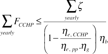
Reference [1] proposes a criteria to increase the full load operation hours until energy saving occurs, or in other words PES ≥ 0 (Figure 6.4). Deriving an equation for this constraint under the following the thermal load (FTL) strategy, discussed in Chapter 1, results in the following equation:
∑yearlyFCCHP≤∑yearlyHdem/(1−ηe, CCHPηe, pp.ηg)ηb
 (6-5)
(6-5)

This means that to satisfy the primary energy saving (PES) constraint under the FTL strategy, Eq. (6-5) should govern.
Considering an energy management strategy such as FTL or following the electricity load (FEL) for the PES constraint while the prime mover size is calculated by MRM seems to be a mistake. The reason is that, for example, when we talk about FTL, it means that the recoverable heat from the engine is sufficient to provide the heating load of the consumer for the whole year. Therefore FTL itself is a sizing method based on the thermal energy management strategy. It is evident that the prime mover size calculated according to MRM is not necessarily equal to the prime mover size that is able to provide all the heating demands during a year (FTL). Therefore the PES constraint proposed by [1] can be modified according to Eq. (6-6) without including any energy management strategy.
∑yearlyFCCHP≤∑yearlyζ(1−ηe, CCHPηe, pp.ηg)ηb
 (6-6)
(6-6)where
ζ={Hdemif Qrec>HdemQrecif Qrec≤Hdem
 (6-7)
(6-7)In Eq. (6-6) it is assumed that the prime mover efficiency ( ηe, CCHP![]() ) in full load operation (FLO) and partial load operation (PLO) equals the nominal electrical efficiency.
) in full load operation (FLO) and partial load operation (PLO) equals the nominal electrical efficiency.
6.3. Developed-MRM
MRM has been further developed into vertical, horizontal, and high-level analysis [2]. These developments are discussed in more detail in the following subsections.
6.3.1. Horizontal Design (Horizontal-MRM)
In this design method, which is very similar to that presented by [1], the full load operation of the prime mover extends until the yearly PES becomes greater than a minimum PES, instead of being positive (Figure 6.5). The prime mover size remains the same as the prime mover size recommended by the classic MRM.

Deriving the equation for the above condition results in the constraint presented in Eq. (6-10):
PES=∑yearlyFpp+∑yearlyFb−∑yearlyFCCHP∑yearlyFpp+∑yearlyFb≥PESmin
 (6-8)
(6-8)
(1−PESmin)∑yearlyηe,CCHPFCCHPηe,ppηg−∑yearlyFCCHP+(1−PESmin)∑yearlyζηb≥0
 (6-9)
(6-9)and finally
∑yearlyFCCHP≤1−PESminηb[1−(1−PESmin)ηe,CCHPηe,ppηg]∑yearlyζ
 (6-10)
The FLO and PLO efficiency of components is assumed to be equal in Eqs. (6-8) to (6-10).
The yearly fuel consumption of the CCHP system ∑yearlyFCCHP is dependent on the operation mode of the prime mover. When the prime mover operates in full load it consumes fuel according to the nominal efficiency, but when it operates in partial load it consumes more fuel and follows its partial load efficiency. Hence
∑yearlyFCCHP=∑FLOFCCHP+∑PLOFCCHP=∑FLOEnomηFLOe,CCHP+∑PLOEPMηPLOe,CCHP
 (6-11)
EPM={EdemEdem≤EnomEnomEdem>Enom
 (6-12)
Depending on the type of prime mover, its electrical efficiency in FLO and PLO conditions ( ηFLOe,CCHP![]() , ηPLOe,CCHP
, ηPLOe,CCHP![]() ) can be found from the data presented in Chapters 1 and 2.
) can be found from the data presented in Chapters 1 and 2.
6.3.2. Vertical Design (Vertical-MRM)
In vertical-MRM, the full load operation time of the prime mover is the same as that recommended by the classic MRM, but the prime mover size becomes greater until the PES remains greater than a minimum PES. Figure 6.5 depicts a graphical explanation of this method.
The equation that can be derived for the vertical-MRM is similar to that derived for the horizontal-MRM in Eqs. (6-10) to (6-12).
In the MRM methods the length of full load operation time may be known (the classic MRM) or unknown (the horizontal-MRM) but the problem is determining the time when the prime mover is supposed to operate in full load or partial load. To determine the time when the prime mover should be programmed for FLO or PLO another constraint should be introduced. This constraint can be based on the cooling, heating, or electrical loads of the consumer. The constraint can also be expressed based on different economic criteria. Moreover, the ability to sell electricity to the grid has an impact on the time for FLO and PLO. In addition, different fuel and electricity tariffs in peak demand and nonpeak demand times can change the constraint. Specifying the constraint depends on the decision-making of the designer. The decision should be made based on evaluations and calculations such as those mentioned in this paragraph.
6.3.3. High-level Analysis
While energy has different aspects such as thermodynamic (energy and exergy), economic, and environmental, both the vertical- and horizontal-MRM sizing methods use only the energy criterion to size the prime mover. The high-level MRM uses the economic criterion of net present value (NPV) after applying the PES constraint. In this method, by changing the prime mover size and full load operation time, the pairs (prime mover size and full load operation time) that result in the same PESmin are found and an iso-PES line is drawn. Then in the second step the NPV criterion is applied to the sizes related to the iso-PES line to find the pair that results in the maximum NPV. The pair with the maximum NPV would be the answer. A graphical representation of the high-level MRM is depicted in Figure 6.6.

The advantage of the high-level MRM is that among different options with the same primary energy savings, the one that creates more economic benefit is chosen as the solution.
6.4. EMS Sizing Methods
Energy management strategies (EMSs) have been used to find better solutions in the sizing of prime movers for CCHP systems[3-9]. The most popular EMS sizing methods include FTL, FEL, and following the seasonal load (FSL). Commonly, researchers have used different strategies to size a CCHP system and then have compared the results from different points of view. The final result depends on the comparisons, investor priorities, and the designer decisions. In the following the details of these sizing methods are introduced.
6.4.1. FTL Sizing
In this method the prime mover size is chosen to provide the maximum thermal demand from the heat recovery of the CCHP system. This means that in case of lack/surplus of electricity it would be purchased/sold from/to the grid respectively. Since the thermal demand changes, the recovered heat from the prime mover may exceed the thermal demand in some conditions. In such conditions the extra heat may be stored in a heat storage system or lost. When working with EMSs, usually FTL is more popular because the extra electricity or lack of electricity can be sold to or bought from the grid and the prime mover also can be programmed to provide the heat demand (no heat lost or storage). In fact in this method the prime mover’s main priority is to produce heat, and electricity is a byproduct of the CCHP system.
EMSs only pay attention to the thermal or electrical loads of the consumer; they pay no attention to other aspects of energy such as the economic and environmental criteria. These criteria may be considered only when comparing different EMS sizing methods to select the best energy management strategy.
A formula for the FLT sizing method is presented here:
EFTLnom={Enom | (B=0∨Qrec=ATDmax)}
where EFTLnom![]() is the nominal size of the prime mover recommended by the FTL sizing method, and B is the auxiliary boiler size to compensate for the lack of heat for different purposes.
is the nominal size of the prime mover recommended by the FTL sizing method, and B is the auxiliary boiler size to compensate for the lack of heat for different purposes.
6.4.2. FEL Sizing
In the FEL sizing method the prime mover size is chosen to provide the maximum electrical demand from the prime mover of the CCHP system. This means that when there is a lack of heat it will be compensated for by an auxiliary heating system such as a water boiler. Since in the FEL sizing method the electricity demand is the main priority of the CCHP system in case of surplus recoverable heat, it is recommended to store the heat in a heat storage system for reuse when needed; otherwise it would be wasted.
When the prime mover is programmed to operate in partial load, no surplus electricity is produced, but if it is supposed to operate in full load, since the electricity demand is changeable, the electricity demand may be less than the full load electricity production of the prime mover. In this case the electricity may be sold to the grid, or be consumed by the auxiliary electrical cooling or heating systems integrated into the CCHP system. Electricity storage systems (batteries) can also be used to store the surplus electricity and sell it to the grid during peak hours when electricity is more expensive. In addition by applying some optimization algorithms the prime mover size can be smaller than the maximum electrical demand and instead electricity storage systems can be used to satisfy the peak demand. This helps to reduce fuel consumption and pollution production, but it may cost more.
The prime mover size in FEL sizing ( EFELnom![]() ) is calculated as follows:
) is calculated as follows:
EFELnom=Edem,max
6.4.3. FSL Sizing
In this method, the prime mover size is designed to follow thermal and electrical loads depending on the monthly or seasonal electricity to heat demand ratio (LR) of the consumer:
LR=Monthly EdemMonthly Hdem
 (6-15)
If LR > 1, the prime mover should be programmed to run in FTL strategy in that month, otherwise it should be programmed to work in FEL strategy. According to this discussion, the prime mover size can be calculated as follows:
EFSLnom=max(EFELnom,EFTLnom)
6.5. Thermodynamic Sizing Methods
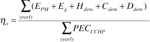
Thermodynamic sizing methods use energy and exergy analyses. In these methods usually the primary energy consumption (PEC) and overall efficiency of the CCHP system are considered as the first law of thermodynamics criteria; also the second law efficiency (π) and exergy destruction ( ˙I![]() ) of the CCHP system are considered as the second law of thermodynamics criteria. In order to find the optimum size of the CCHP systems from the energy point of view the Eqs. (6-17) and (6-18) must be maximized:
) of the CCHP system are considered as the second law of thermodynamics criteria. In order to find the optimum size of the CCHP systems from the energy point of view the Eqs. (6-17) and (6-18) must be maximized:
FESR=∑yearlyPECSCHP−∑yearlyPECCCHP∑yearlyPECSCHP
 (6-17)
ηo=∑yearly(EPM+Eg+Hdem+Cdem+Ddem)∑yearlyPECCCHP
 (6-18)
where
Eg={0 if EPM≥EdemEdem−EPM if EPM<Edem
 (6-19)
where PEC is the fuel energy consumption to provide all energy demand types for the consumer. EPM and Eg are the electricity produced by the prime mover and electricity purchased from the grid, respectively. Using FESR as the energy criterion is common in the research; we also recommend using this criterion since it compares the fuel consumption of the CCHP with the SCHP system as well.
In order to find the optimum CCHP size from the exergy point of view the Eqs. (6-20) and (6-21) must be maximized:
EXIR=πCCHP−πSCHPπCCHP
 (6-20)
˙IRR=˙ISCHP−˙ICCHP˙ISCHP
 (6-21)
where EXIR and ˙IRR![]() stand for exergy efficiency increase ratio, and exergy destruction reduction ratio, respectively. In addition π and ˙I
stand for exergy efficiency increase ratio, and exergy destruction reduction ratio, respectively. In addition π and ˙I![]() should be calculated yearly as follows:
should be calculated yearly as follows:
π=∑yearly˙ϕout∑yearly˙ϕin
 (6-22)
˙I=∑yearly˙ϕin−∑yearly˙ϕout
 (6-23)
where ˙ϕin![]() and ˙ϕout
and ˙ϕout![]() are the supplied and recovered exergy rate. Guides for calculation of ˙ϕ
are the supplied and recovered exergy rate. Guides for calculation of ˙ϕ![]() are given in Chapter 3.
are given in Chapter 3.
Exergy and energy criteria usually result in different optimum sizes for the CCHP system. Therefore, if we are supposed to use both energy and exergy criteria simultaneously, we must compromise between the two points of view in order to propose a single optimum size.
A solution for this problem is to introduce another function that is a linear combination of the energy and exergy criteria. For example, if we have decided to use FESR and EXIR simultaneously for sizing, the following equation can be maximized:
ENEX=ωENFESR+ωEXEXIRωEN+ωEX=10≤ωEN,ωEX≤1
 (6-24)
where ωEN and ωEX are the energy and exergy weights, respectively, and ENEX stands for energy/exergy function.
Another solution is to determine the optimum size recommended by every criterion independently and then combine the optimum sizes linearly as follows:
EENEXnom=ωENEFESRnom+ωEXEEXIRnomωEN+ωEX=10≤ωEN,ωEX≤1
 (6-25)
The CCHP size proposed by Eqs. (6-24) and (6-25) usually maximizes neither FESR nor EXIR; in fact it is a compromise between energy and exergy criteria.
While calculating the thermodynamic criteria, attention must be paid to the operation mode of the prime mover. According to the analyses one decide to operate it in partial load, full load, or a combination of PLO and FLO during the course of a year.
In addition it should be fully understood that it is unfeasible to reuse all of the recoverable heat from the prime mover due to the highly changeable heating and cooling demands. Therefore any calculation should be done according to the energy demands of the consumer. It is evident that the selling or saving of the surplus electricity produced by the prime mover (if it exists) should be decided according to the economic evaluations. Thermodynamic sizing methods cannot help in decisions about such problems alone. This weakness of thermodynamic analyses is eliminated in the thermoeconomical sizing methods presented in the following.
6.6. Thermoeconomic Sizing Methods
In thermoeconomic analyses, in addition to thermodynamic analyses, the economic aspect of energy and energy conversion equipment is also considered. In the literature review presented in Chapter 1 many economic criteria that have been used by researchers were introduced. Table 1.1 summarized the economic criteria into four categories of present value methods, rate of return methods, ratio methods, and payback methods. The most commonly used criteria from each category are the net present value (NPV), internal rate of return (IRR), premium value percentage (PVP), and payback period (PB).
The NPV calculates the real value of the project after its lifetime (L), in other words it tells us if the project will be profitable during its lifetime or not. NPV can be calculated as follows:
NPV=−I+SV(1+r)L+∑Ly=1cfy(1+r)y
 (6-26)
where r is the interest rate, and I is the initial capital cost of the CCHP system and includes every cost before operation such as the costs of a consultant, hardware, transportation, installation, tests, site rent, labor, tax, etc.
cfy is the annual net cash, the annual summation of every positive and negative cash flow after operation during the lifetime of the project (cfy = (er − ex)y). The positive cash flow, which means earnings (er) includes the yearly costs that are not paid in comparison with the SCHP system, such as the electricity provided by the CCHP system, the heating, DHW, or cooling provided by heat recovery, and electricity sold back to the grid. The negative cash flow mean expenses (ex), including yearly costs paid for operation, maintenance, and meeting consumer demands. These expenses may include the costs of fixed and variable O&M, taxes, fuel, and electricity purchased from the grid. SV is the salvage value of the project after its lifetime.
Positive NPV means profitability and in the sizing process the CCHP size with the maximum NPV is the most profitable CCHP.
According to Eq. (6-26) the bigger the annual net cash flow (cfy) is, the more positive NPV would be. In addition a smaller initial capital cost (I) increases the NPV.
Due to the importance of cfy some designers [3, 10–13] have preferred to optimize this parameter or its components such as annual costs, avoided costs, annual savings, etc.
In the NPV methods attention is not paid to the interest rate and economic situation of the country where the investment takes place. The same projects respond differently from the economic point of view in countries with different economic situations. For this reason, there must be a tool to evaluate the risk of investment. IRR is very useful for this purpose. IRR is the interest rate at which the profitability of the project is zero. The bigger the IRR is, the safer the investment will be. IRR can be calculated according to the following equation:
−I+SV(1+IRR)L+∑Ly=1cfy(1+IRR)y=0
 (6-27)
A CCHP size is profitable when IRR is greater than the interest rate r. The larger the profitability margin (IRR − r) is, the lower the risk of investment will be. In unstable economics, a minimum profitability margin should be considered to decrease the risk of investment.
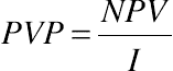
If we are required to know the net profit for every dollar of investment in different sizes of CCHP system, the premium value percentage (PVP) should be calculated as follows:
PVP=NPVI
 (6-28)
The CCHP size with the highest PVP is the best. For calculation of the PVP, the NPV must be positive.
Another criterion that is easily understandable, especially for nonexpert investors, is the payback period (PB). This criterion calculates the number of years it takes to recover the original capital cost. It is important to mention that this criterion does not calculate the years it takes to recover the real value of the investment cost, because it does not consider the interest rate. It means that if you have invested 1 USD today you will receive exactly 1 USD after the payback period. This criterion is sometime misleading because it may calculate the payback period while the NPV is negative. This is due to neglecting the impact of interest rate in calculating the PB. PB can be calculated as follows:
PB=I¯cf
 (6-29)
where ¯cf=1L∑Ly=1cfy is the yearly average net cash flow. In order to avoid a misleading PB and incorrect decision-making, we propose a modified payback period equation:
PB′=LINPV+I=L1PVP+1
 (6-30)
This equation predicts the payback period more realistically than Eq. (6-29) because it considers the real value of the profit (NPV) in the calculations.
In addition to the above criteria, levelized electricity production cost (LEPC) can also be considered as a design criterion. This criterion calculates the cost per kilowatt of electricity production in the CCHP system. A smaller LEPC means a more efficient CCHP system thermoeconomically. LEPC can be calculated according to Eq. (1-17).
6.7. Multicriteria Sizing Methods
Since energy has different aspects, optimizing one aspect may decrease the benefits of others. In addition, when we need to consider other characteristics of energy and CCHP systems such as the environmental impact, the problem will become more complex and designing a CCHP system with optimum design criteria from different points of view becomes unfeasible. Due to the importance of different characteristics of energy and CCHP systems, none of the criteria can be omitted or neglected; therefore a solution should be proposed to consider all of these characteristics. Researchers have proposed the fitness function (ff) and multicriteria sizing function (MCSF). In the following sections these methods are further explained and expanded upon in the context of sizing CCHP systems.
6.7.1. Fitness Function Sizing Method
References [11] and [14] used a fitness function to design CCHP systems. A sample of the ff is presented in Eq. (1-36). By looking at this equation we can see that FESR, annual total cost savings (ATCS), and CO2 reduction ratio are considered as the nominated criteria of the thermodynamic, economic, and environmental aspects of the energy and CCHP system, respectively. In addition, an equal weight is given to the three criteria. To expand upon this method, we propose considering some criteria that each have several subcriteria. In addition, the weight of every criterion and subcriterion can be calculated using weighting methods such as AHP or the fuzzy method presented in Chapter 4. The fitness function is formulated as follows:
ff=∑ni=1wiffi,∑nI=1wi=1
 (6-31)
where
ffi=∑kij=1βijwijCij∑ni=1∑kij=1wij=1βij={1 if the Cij is considered in the analyses0 if the Cij is not considered in the analyses
 (6-32)
where n is the number of criteria and ki is the number of subcriteria of the ith criterion. In addition wi is the weight of ith criterion and wij is the weight of the jth subcriterion of the ith criteria. Cij is the normalization of the jth subcriterion of the ith criteria. According to the normalization method, the optimization may be done by maximizing or minimizing the ff. The Cij is defined as follows:
Cij=cCCHPij−cSCHPijcCCHPij, cij>0
 (6-33)
where cij is a profit such as the exergy efficiency where higher the better.
If cij is a cost such as the fuel consumption where smaller the better, it would be normalized as follows:
Cij=cSCHPij−cCCHPijcSCHPij, cij>0
 (6-34)
Equation (6-31) can be optimized by using different optimization algorithms such as the genetic algorithm. As mentioned previously, the weights of the criteria and subcriteria should be calculated using the weighting methods presented in Chapter 4.
It is important to mention that optimizing the fitness function does not guarantee the optimization of every criteria or subcriteria. In fact the weakness of this method is that the optimum ff may result in some nonoptimum criteria or subcriteria, even those that are most important for the designer. This is because when the ff is being optimized we have no control on the variation of ffi and Cij.
Another weakness of this method is that some of the subcriteria may be steadily increasing or decreasing. Such subcriteria may cause the ff to become steadily increasing or decreasing. In such cases, since we optimize all of the subcriteria together, all of the subcriteria should be checked individually and we should find the subcriterion (or criteria) that caused this divergence. The designer may make different decisions about the subcriteria that are to blame; for example their weight can be set to zero, another subcriterion can be used instead, another sizing method can be used, etc.
6.7.2. Multicriteria Sizing Function
The MCSF proposed by [15] optimizes every subcriterion of Cij individually and finds the optimum CCHP size proposed by the subcriterion. Then after giving weight to every criterion and subcriterion, a linear combination of weights and optimum CCHP sizes proposed by the sub-criteria is calculated, and the prime mover size of the CCHP system is recommended as follows:
EMCSFnom=∑ni=1∑kij=1βijωiωijEijopt
 (6-35)
Eijopt={Enom| Cij(Enom, Conditions)|opt, i=1,…,n & j=1,2,…,ki}
 (6-36)
where Eijopt![]() is the optimum CCHP size, or the proposed CCHP size under some conditions and constraints from the jth sub-criterion of the ith criterion, and EMCSFnom
is the optimum CCHP size, or the proposed CCHP size under some conditions and constraints from the jth sub-criterion of the ith criterion, and EMCSFnom![]() is the nominal electrical capacity of the prime mover proposed by the MCSF.
is the nominal electrical capacity of the prime mover proposed by the MCSF.
As we discussed previously, in problems such as CCHP sizing where many criteria are encountered, it is basically impossible to find a CCHP size to optimize all of the criteria and subcriteria simultaneously. Therefore we should look for a compromise or quasi-optimum solution. In comparison with the ff method, the MCSF has absolute control over the optimization of every subcriterion. Therefore, EMCSFnom![]() tends to approach the size of Eijopt
tends to approach the size of Eijopt![]() for which the corresponding criterion and subcriterion is the most important (has the biggest ωiωij) for the designer. In addition, since all of the subcriteria are optimized individually, if there is a subcriterion that is steadily increasing or decreasing, we can use our engineering feelings about the problem and according to the trend of the subcriterion reach an agreement about the recommended engine size from that subcriterion. This means we may use the optimum sizes of some criteria and the agreed sizes proposed by some nonoptimizable subcriteria in the MCSF. In other words, with the MCSF there is always a solution.
for which the corresponding criterion and subcriterion is the most important (has the biggest ωiωij) for the designer. In addition, since all of the subcriteria are optimized individually, if there is a subcriterion that is steadily increasing or decreasing, we can use our engineering feelings about the problem and according to the trend of the subcriterion reach an agreement about the recommended engine size from that subcriterion. This means we may use the optimum sizes of some criteria and the agreed sizes proposed by some nonoptimizable subcriteria in the MCSF. In other words, with the MCSF there is always a solution.
6.8. Case Study
Design a CCHP system to provide the energy demands of the building described in the previous chapter. Use MRM, EMS, ff, and MCSF, and compare the results of the methods. In addition, show the impact of climate difference on the design of the CCHP cycle for the five climates presented in Chapter 5. Assume that the prime mover is operating at full load the whole year and that the DHW system is prepared by heat recovery. The economic, environmental, and technical input data for the written code are presented in Appendix 2[13, 16-33].
6.8.1. Solution Outline
In order to design a CCHP system, first we should decide upon the prime mover type. The prime mover was previously chosen based on the multicriteria decision-making method in Chapter 4 for the five climates. The fuzzy logic and grey incidence approaches recommended using an internal combustion (IC) engine for all five climates. In the second step, the energy demands of the residential building were calculated and presented in Chapter 5. In the third step, the components (apart from the internal combustion engine) that are supposed to be used in the CCHP cycle should be introduced as a basic CCHP system. Since the exhaust gas of an IC engine is about 540 °C, this energy source can be used for cooling production in single-effect absorption chillers. The water is preheated by the lube oil cooler and engine water jacketing before being heated by the exhaust gases. If the water temperature is high enough for the chiller to cover the cooling load (or heating load), the temperature control valve (TCV) bypasses the hot water to the down stream of auxiliary boiler and it enters the chiller (or heating system), otherwise it will be reheated by the auxiliary heater. The CCHP cycle consisting of the IC engine, absorption chiller, auxiliary heater, and heating system are presented in Figure 6.7. Determining the prime mover size dictates the size of the auxiliary boiler. In addition, the chiller size is determined according to the maximum cooling load. Therefore the IC engine should be sized first.

6.8.2. Sizing Using the MRM
The ATD of the building is first determined using the MRM method. The ATD curves of the building for the five climates are depicted in Figure 6.8. Since the load calculation was done based on the TNM, the horizontal axis of ATD curves is presented in percent time of year.
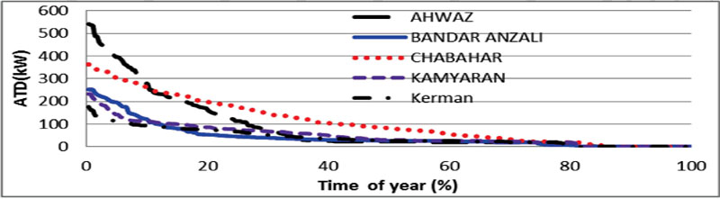
After determining the ATD, the rectangle with maximum area and FLO time should be found for every climate. For our purposes, the area of the rectangle is calculated against the time of year in Figure 6.9. The IC engine size can be found by using the maximum area and its corresponding FLO time in Eq. (6-3). The results of sizing using the MRM are presented in Figure 6.10.


6.8.3. Sizing Using EMS Methods
EMS sizing methods including the FTL, FEL, and FSS can also be used for sizing the IC engine according to Eqs. (6-13), (6-14), and (6-16). In these methods it is enough to determine the peak of ATD and the electrical demand for every climate. In the FTL sizing method the engine size should be chosen to provide as much recoverable heat as ATDmax. Therefore the correlations that were presented for Qrec and Enom of the IC engine in the second chapter can be used to calculate the engine size. For example, Eq. (2-10) is used in this example since the electrical demand is below 100 kW. As an example the ATDmax of Ahwaz is 541.40 kW, therefore by using Eq. (2-10) we have 541.40 = 1.368Enom + 14.57 or Enom = 385.11 kW. The results of the EMS for the five climates are presented in Figure 6.10 and compared with the MRM results.
As can be seen among the sizing methods, the FTL and FSL approaches recommend the biggest engine size. A bigger engine size means a higher initial investment cost and more heat loss since the recoverable heat high enough to cover the maximum aggregated thermal demand (it means heat is wasted when the ATD decreases). In addition, operation and maintenance of a bigger engine costs more. The positive side of a bigger engine is production of surplus electricity to be sold to the grid and no need for an auxiliary boiler. These can improve the economic benefits of the CCHP system. As can be seen many parameters are interacting with each other and the final decision can only be made when all of the vital criteria and subcriteria are calculated. As opposed to the FTL and FSL, the engine sizes proposed by the FEL are small. A small engine size has its own characteristics as well. For example, smaller initial capital outlay, and lower operation and maintenance costs are the advantages, while the need for an auxiliary boiler and less excess electricity to be sold to the grid can be mentioned as disadvantages. In contrast to the EMS sizing methods, in most cases MRM proposes intermediate engine sizes with respect to those proposed by the FTL, FSL, and FEL sizing methods. The intermediate engine size benefits from the advantages of small and big engine sizes, however again the final decision can only be made when all of the essential criteria are calculated. This means that using the MRM or EMS sizing methods without including thermodynamic, economic, and environmental criteria is risky.
Another weakness of the MRM and EMS sizing methods is that they are completely building-demand oriented and do not consider the impact from the components of the CCHP system. For example if using MRM or EMS as sizing methods there will be no difference between the size of the prime mover of a basic CCHP and a CCHP system that is integrated with solar heating or a thermal storage system.
6.8.4. Sizing Using ff
In order to use ff for sizing the IC engine, the criteria, subcriteria, and their weights should be known.
In this example we consider FESR and EXIR as the thermodynamic subcriteria; NPV, IRR and PB as the economic subcriteria; and the reduction ratio of CO2, CO, and NOx as the environmental subcriteria. The AHP weighting method is used and most of the pairwise comparisons presented in Chapter 4 (Tables 4.7A, B, and D) can be used again except for the economic subcriteria (Table 4.7C) due to consideration of different subcriteria. The pairwise comparison of economic subcriteria and weights are presented in Tables 6.1 and 6.2 , respectively.
Table 6.1
Pairwise Comparison of Economic Subcriteria
| NPV | IRR | PB | |
| NPV | JE | WMI | SMI(R) |
| IRR | WMI(R) | JE | VSMI(R) |
| PB | SMI | VSMI | JE |

Table 6.2
Weights of Criteria and Subcriteria Considered for Sizing
| Criteria | Weight | Subcriteria | Weight |
| Thermodynamic | 0.34 | FESR (c11) | 0.55 |
| EXIR(c12) | 0.45 | ||
| Environmental | 0.20 | CORR(c21) | 0.29 |
| CO2RR(c22) | 0.33 | ||
| NOXRR(c23) | 0.38 | ||
| Economic | 0.46 | NPV(c31) | 0.33 |
| IRR(c32) | 0.50 | ||
| PB(c33) | 0.17 |

After calculating the weights, the subcriteria should be calculated according to Eqs. (6-33) and (6-34). Among the subcriteria, FESR, CO2RR, CORR, and NOXRR should be normalized according to Eq. (6-34) and EXIR should be normalized according to Eq. (6-33). The economic subcriteria, however, cannot be normalized using Eqs. (6-33) and (6-34). This is because the net annual cash flow (cfy) is always negative for the SCHP system, and as a result the NPV, IRR, and PB would become negative (meaningless). This is because we receive no economic benefit from the SCHP system. For this reason NPV, IRR, and PB are normalized as follows:
C31={cCCHP31/(cCCHP31−cSCHP31),if cCCHP31>00,if cCCHP31≤0
 (6-37)
C32={(cCCHP32−r)/cCCHP31,if cCCHP32>r0,if cCCHP32≤r
 (6-38)
C33={1/cCCHP33,if0<¯cf<ICCHP1,ifICCHP<¯cf0,if¯cf≤0
 (6-39)
To calculate the Cij, we should calculate the cij first. For this purpose in the following all of the subcriteria are formulated according to the cycle presented.
The first subcriterion is the fuel consumption of the CCHP and SCHP systems. To present the following equations in a compact form, whenever j is used as a superscript it can take two values of j = 0 or j = 1, in which 0 represents the SCHP system and 1 stands for a CCHP system. In addition an energy vector including four components (E, C, H, and D) is used for the electricity, cooling, heating, and DHW demands. This vector is also used for other subcriteria. Hence
Fj=(FjE,FjC,FjH,FjD), j=0, 1
cj11=∑yearly(FjE+FjC+FjH+FjD)
 (6-41)
where the fuel vector components are calculated as follows:
F0E=Edemηppηg,F1E=EPM+QrecηCHP+(E′dem)ηppηgF0C=CdemηbCOPabcɛFCU,F1C=C′demηbCOPabcɛFCUF0H=HdemηbɛFCU,F1H=H′demηbɛFCUF0D=Ddemηwh,F1D=Ddemηwh
 (6-42)
where
EPM={Enom, if FLOEdem, if Enom≥Edem ∧PLOEnom, if Enom<Edem ∧PLOQrec={1.368EPM+14.57,30≤E(kW)≤5001.854EPM, 0≤E(kW)<30E′dem={Edem−EPM,if Edem>EPM0,if Edem≤EPMC′dem={Cdem−COPabcQrs,if Cdem>COPabcQrs0,if Cdem≤COPabcQrsH′dem={Hdem−Qrs,if Hdem>Qrs0,if Hdem≤QrsQrs=Qrec+Qsolar
 (6-43)
Since the DHW energy demand is calculated separately, the CCHP system can be designed with a separate DHW system (sprt-DHW) or be integrated with the heating system and use the recovered heat (intg-DHW). In this example the intg-DHW system is used and the DHW energy demand is combined with the heating energy demand. The prime (′) in the above equations represents the additional energy required (heat from the auxiliary boiler or electricity from the grid) to provide the corresponding energy demand for the building. Qsolar, which is the solar energy collected by a solar water heater, will be calculated in the next chapter.
Since the engine is supposed to operate at full load all time, the recoverable heat may exceed the heat demand at some particular times. The extra heat will be wasted because no heat storage is considered to store the surplus heat. In order to calculate the annual energy loss of the CCHP system the following equation can be used:
ATD≤Qrs→HCCHPloss=Qrs−ATD
Additionally, sometimes the heat demand (for cooling or heating) may exceed the recoverable heat. In this case the lack of heat should be compensated for by burning fuel in the auxiliary boiler and water heater (for the sprt-DHW). The annual lack of heat that should be provided by systems other than the solar and heat recovery systems can be calculated as follows:
ATD≥Qrs→ATD′=H′dem+C′dem/COPabc+Ddem
After calculation of fuel consumption for the CCHP and SCHP systems, the FESR can be calculated according to Eq. (6-34).
In the exergy analysis, the supplied exergy to ( ˙ϕin![]() ) and recovered exergy from ( ˙ϕout
) and recovered exergy from ( ˙ϕout![]() ) the CCHP and SCHP systems are used to calculate the exergy efficiency (π) as follows:
) the CCHP and SCHP systems are used to calculate the exergy efficiency (π) as follows:
˙ϕjin=(˙ϕjin,E,˙ϕjin,C,˙ϕjin,H,˙ϕjin,D)˙ϕjout=(˙ϕjout,E,˙ϕjout,C,˙ϕjout,H,˙ϕjout,D)
 (6-46)
πj=∑yearly(˙ϕjout)/∑yearly(˙ϕjin)
 (6-47)
The exergy vector components are calculated according to the cycle as follows:
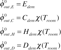
˙ϕ0in,E=F0Eχ(Thg)−(F0E−Edem)χ(Tamb)˙ϕ0in,C=˙Wsp+˙Wrp+˙Wwp+F0Cχ(Thg)−F0C(1−ηb)χ(Tamb)˙ϕ0in,H=˙Wwp+F0Hχ(Thg)−F0H(1−ηb)χ(Tamb)˙ϕ0in,D=F0Dχ(Thg)−F0D(1−ηb)χ(Tamb)
 (6-48)
˙ϕ0out,E=Edem˙ϕ0out,C=Cdemχ(Troom)˙ϕ0out,H=Hdemχ(Troom)˙ϕ0out,D=Ddemχ(Troom)
 (6-49)
˙ϕ1in,E=F1Eχ(Thg)−(F1E−EPM−Qrec)χ(Tamb)+E′dem˙ϕ1in,C=˙Wsp+˙Wrp+˙Wwp+F1Cχ(Thg)−F1C(1−ηb)χ(Tamb)˙ϕ1in,H=˙Wwp+F1Hχ(Thg)−F1H(1−ηb)χ(Tamb)˙ϕ1in,D=F1Dχ(Thg)−F1D(1−ηb)χ(Tamb)
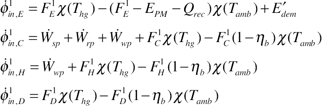 (6-50)
˙ϕ1out,E=EPM+E′dem+˙ϕQrs˙ϕ1out,C′=C′demχ(Troom)˙ϕ1out,H′=H′demχ(Troom)˙ϕ1out,D=Ddemχ(Troom)
 (6-51)
where ambient temperature is calculated according to the weather information presented in Chapter 5:
Tamb={Tdb,sumif (Hdem=0∧Cdem≠0)Tdb,winif (Cdem=0∧Hdem≠0)Troomif Hdem=Cdem=0
 (6-52)
Troom={Troom,sumif (Cdem=0∧Hdem≠0)Troom,winif (Hdem=0∧Cdem≠0)Tambif Hdem=Cdem=0
 (6-53)
χ(Tx)=1−T0/Tx
Since Qrs comprises the recovered heat from the oil cooler, water jacketing, exhaust, and solar system, its exergy is calculated as follows:
Qrs=Qoil+Qjacketing+Qexhaust+Qsolar→˙ϕQrs=Qoilχ(Toil)+Qjacketingχ(Tjacketing)+Qexhaustχ(Texhaust)+Qsolarχ(Tp)
 (6-54)
After calculating the exergy efficiency the EXIR can be calculated according to Eq. (6-33).
In order to investigate the environmental impact of the CCHP with respect to the SCHP system the pollution product by the energy demand components should be evaluated. The pollution vector is defined as follows:
Xj=(XjE,XjC,XjH,XjD)
where X can be CO, CO2, or NOx. The emission production of each pollutant also is determined as follows:
EmjX=∑yearly(XjE+XjC+XjH+XjD)t
 (6-56)
The components of the pollution vector are calculated as follows:
X0E=EPM⋅i0X, E, X0C=Cdem⋅i0X, CX0H=Hdem⋅i0X, H, X0D=Ddem⋅i0X, D
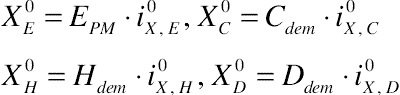 (6-57)
X1E=EPM⋅i1X, E+E′dem⋅i0X, E, X1C=C′dem⋅i1X, CX1H=H′dem⋅i1X, H, X1D=Ddem⋅i1X, D
 (6-58)
where i is the pollution index based on kg/MWh. After calculation of EmjX![]() for each pollutant, the emission reduction ratio can be calculated according to Eq. (6-34).
for each pollutant, the emission reduction ratio can be calculated according to Eq. (6-34).
In the economic evaluations, the initial investment cost and net annual cash flow are the key parameters. Initial investment cost is the summation of equipment costs. The capital cost vector and investment cost are presented as follows:
Ij=(IjE,IjC,IjH,IjD)
Ij=IjE+IjC+IjH+IjD
The capital vector components are calculated as follows:
I0E=NOU.i0E, I1E=Enom⋅i1E+I0E
I0C=Cnom⋅i0C, I1C=Cnom⋅i1CCnom=max(Cdem)
 (6-62)
I0H=B0⋅i0H, B0=maxmax(Hdem, Cdem/COPabc)I1H=B1⋅i1H+Aco⋅i1solar, B1=maxmax(H′dem, C′dem/COPabc)
 (6-63)
I0D=I1D={NOU×iDsprt−DHW0intg−DHW
 (6-64)
where i is the price index in currency-unit/kW (for example USD/kW) except for i0E![]() which is in currency-unit/NOU. NOU means the number of units in the building (each unit has an electricity counter) to measure the electricity flow from the grid to the building. B, Cnom, and Aco are the nominal capacity of the boiler, chiller, and the solar collector area, respectively.
which is in currency-unit/NOU. NOU means the number of units in the building (each unit has an electricity counter) to measure the electricity flow from the grid to the building. B, Cnom, and Aco are the nominal capacity of the boiler, chiller, and the solar collector area, respectively.
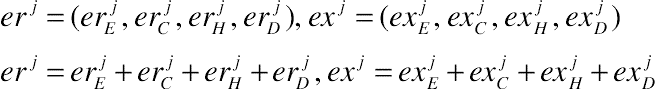
The net annual cash flow calculation starts with determining the earnings (positive cash flow) and expenses (negative cash flow). The earning (er) and expense (ex) vectors and the net annual cash flow (cfy) are presented here:
erj=(erjE, erjC, erjH, erjD), exj=(exjE, exjC, exjH, exjD)erj=erjE+erjC+erjH+erjD, exj=exjE+exjC+exjH+exjD
 (6-65)
cfjy=−IjOM+(erj−exj)y
where IjOM![]() is the yearly operation and maintenance costs. The components of the earning and expense vectors are formulated below:
is the yearly operation and maintenance costs. The components of the earning and expense vectors are formulated below:
er0E=0, ex0E=Edem⋅tbeer0C=0, ex0C=F0C⋅tgaser0H=0, ex0H=F0H⋅tgaser0D=0, ex0D=F0D⋅tgas
 (6-67)
er1E={Edem⋅tbe+(EPM−Edem)⋅tseEPM≥EdemEPM⋅tbeEPM<Edemex1E=(F1E−(E′dem)ηppηg)⋅tgas+E′dem×tbeer1C=(F0C−F1C)⋅tgas, ex1C=F1C⋅tgaser1H=(F0H−F1H)⋅tgas, ex1H=F1H⋅tgaser1D=0, ex1D=F1D⋅tgas
 (6-68)
where t is a tariff and the subscripts of gas, se, and be stand for natural gas, selling electricity, and buying electricity. EPM is the electrical output of the engine and should not be mistaken with Enom.
After calculation of I and cfy the economic criteria of NPV, IRR, and PB can be calculated according to Eqs. (6-26), (6-27), and (6-29), respectively. Also these criteria can be normalized according to Eqs. (6-37) to (6-39), respectively.
Up to now we have formulated all of the subcriteria. By combining these criteria and the corresponding weights in the fitness function (Eq. 6-31) the magnitude of ff can be drawn against the engine nominal size (Enom) as in Figure 6.11. As can be seen in Figure 6.11 the ff for all five climates has an optimum point and reaches a maximum. The optimum sizes for the five climates are given in Figure 6.10 for comparison with other sizing methods. In addition, the results presented in figure 6.12 shows that every criterion for the climate of Kamyaran has an optimum point. According to the sizes proposed by ff and comparing them with the sizes proposed by the MRM and EMS for the climate of Kamyaran, it can be seen from Figure 6.13 that using MRM and FEL give smaller subcriteria in most cases except for C22 and C11. In addition, in comparison with the ff, using FTL and FSL results in smaller or equal values for all of the subcriteria. It should be noted that using the MRM or EMS sizing methods may result in economically unbeneficial CCHP systems (see the C31, C32 for Kamyaran when using the FEL sizing method). Furthermore, Figure 6.13 reveals that EXIR has no optimum point and is increasing steadily, but fortunately combining it with FESR results in ff1, which has an optimum point (Figure 6.12).


6.8.5. Sizing Using MCSF
The MCSF and ff methods have many parts in common except in the method they use to calculate the optimum size. The subcriteria calculated in the ff method are used to calculate the optimum or proposed engine size for every subcriterion. An example of the subcriterion is depicted for the climate of Kamyaran in Figure 6.13. As can be seen, except for C12 there are optimum sizes for each subcriterion. Regarding C12, according to the trend of EXIR we have assumed an EXIR of 90% as the design constraint for this subcriterion. After calculating the engine sizes proposed by the subcriteria, they are combined with the weights in Eq. (6-35) to calculate the final size (Figure 6.10). In comparison with the ff, the sizes proposed by the MCSF are smaller in all climates. Smaller engine sizes mean a smaller initial investment. This smaller capital cost does not guarantee the profitability of the CCHP system. This should be checked according to the subcriteria curves that are presented in Figures 6.14 to 6.21 . In addition the profitability of the sizes that were proposed by other sizing methods can be checked with these curves. The chiller size only depends on the maximum cooling load for every climate, but the boiler size depends on the engine size and building demands. The boiler size is plotted against Enom in Figure 6.22, which can be used for both ff and MCSF. Table 6.3 presents the boiler and chiller sizes when designing with MCSF.


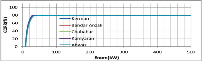


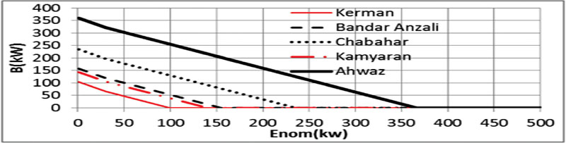
Table 6.3
The Absorption Chiller Boiler Size for Different Climates Using MCSF
| Kerman | Ahwaz | Bandar Anzali | Chabahar | Kamyaran | |
| Chiller size (kW) | 105 | 361 | 159 | 236 | 145 |
| Boiler size (kW) | 52 | 183 | 76 | 117 | 81 |

6.9. Problems
1. Use the building demands calculated in previous chapter problems to calculate the ATD of the building.
2. By using the MRM design a CCHP system for your case study.
3. Use horizontal-MRM and vertical-MRM to design the CCHP system and compare the results from the economic point of view.
4. What would be the size of the engine if you use high-level analysis instead of MRM?
5. Design the CCHP system using the EMS.
6. Use MCSF and ff to design the CCHP for the building you have considered.
7. If the CCHP is supposed to use a combination of electrical and absorption chillers, modify the formulations for this change.
8. If the CCHP is supposed to use a thermal storage system, draw the schematic of the new CCHP system.
9. Modify the formulations for the new CCHP system you have drawn in the Problem 8.
10. The price of electricity is usually higher at peak hours. Evaluate if it is profitable to use an electricity storage system to store electricity at low load hours and sell it in peak hours or not. Calculate the PB and NPV of this idea.