
CHAPTER 1
COMPUTATIONAL INTELLIGENCE: FOUNDATIONS, PERSPECTIVES, AND RECENT TRENDS
The field of computational intelligence has evolved with the objective of developing machines that can think like humans. As evident, the ultimate achievement in this field would be to mimic or exceed human cognitive capabilities including reasoning, understanding, learning, and so on. Computational intelligence includes neural networks, fuzzy inference systems, global optimization algorithms, probabilistic computing, swarm intelligence, and so on. This chapter introduces the fundamental aspects of the key components of modern computational intelligence. It presents a comprehensive overview of various tools of computational intelligence (e.g., fuzzy logic, neural network, genetic algorithm, belief network, chaos theory, computational learning theory, and artificial life). The synergistic behavior of the above tools on many occasions far exceeds their individual performance. A discussion on the synergistic behavior of neuro-fuzzy, neuro-genetic algorithms (GA), neuro-belief, and fuzzy-belief network models is also included in the chapter.
1.1 WHAT IS COMPUTATIONAL INTELLIGENCE?
Machine Intelligence refers back to 1936, when Turing proposed the idea of a universal mathematics machine [1,2], a theoretical concept in the mathematical theory of computability. Turing and Post independently proved that determining the decidability of mathematical propositions is equivalent to asking what sorts of sequences of a finite number of symbols can be recognized by an abstract machine with a finite set of instructions. Such a mechanism is now known as a Turing machine [3]. Turing’s research paper addresses the question of machine intelligence, assessing the arguments against the possibility of creating an intelligent computing machine and suggesting answers to those arguments, proposing the Turing test as an empirical test of intelligence [4]. The Turing test, called the imitation game by Turing, measures the performance of a machine against that of a human being. The machine and a human (A) are placed in two rooms. A third person, designated the interrogator, is in a room apart from both the machine and the human (A). The interrogator cannot see or speak directly to either (A) or the machine, communicating with them solely through some text messages or even a chat window. The task of the interrogator is to distinguish between the human and the computer on the basis of questions he/she may put to both of them over the terminals. If the interrogator cannot distinguish the machine from the human then, Turing argues, the machine may be assumed to be intelligent. In the 1960s, computers failed to pass the Turing test due to the low-processing speed of the computers.
The last few decades have seen a new era of artificial intelligence focusing on the principles, theoretical aspects, and design methodology of algorithms gleaned from nature. Examples are artificial neural networks inspired by mammalian neural systems, evolutionary computation inspired by natural selection in biology, simulated annealing inspired by thermodynamics principles and swarm intelligence inspired by collective behavior of insects or micro-organisms, and so on, interacting locally with their environment causing coherent functional global patterns to emerge. These techniques have found their way in solving real-world problems in science, business, technology, and commerce.
Computational Intelligence (CI) [5–8] is a well-established paradigm, where new theories with a sound biological understanding have been evolving. The current experimental systems have many of the characteristics of biological computers (brains in other words) and are beginning to be built to perform a variety of tasks that are difficult or impossible to do with conventional computers. To name a few, we have microwave ovens, washing machines, and digital cameras that can figure out on their own what settings to use to perform their tasks optimally with reasoning capability, make intelligent decisions, and learn from the experience. As usual, defining CI is not an easy task. Bezdek defined a computationally intelligent system [5] in the following way:
“A system is computationally intelligent when it: deals with only numerical (low-level) data, has pattern recognition components, does not use knowledge in the AI sense; and additionally when it (begins to) exhibit i) computational adaptivity, ii) computational fault tolerance, iii) speed approaching human-like turnaround and iv) error rates that approximate human performance.”
The above definition infers that a computationally intelligent system should be characterized by the capability of computational adaptation, fault tolerance, high computational speed, and be less error prone to noisy information sources. It also implies high computational speed and less error rates than human beings. It is true that a high computational speed may sometimes yield a poor accuracy in the results. Fuzzy logic and neural nets that support a high degree of parallelism usually have a fast response to input excitations. Further, unlike a conventional production (rule-based) system, where only a single rule is fired at a time, fuzzy logic allows firing of a large number of rules ensuring partial matching of the available facts with the antecedent clauses of those rules. Thus the reasoning capability of fuzzy logic is humanlike, and consequently it is less error prone. An artificial neural network (ANN) also allows firing of a number of neurons concurrently. Thus it has a high computational speed; it usually adapts its parameters by satisfying a set of constraints that minimizes the error rate. The parallel realization of GA and belief networks for the same reason have a good computational speed, and their inherent information filtering behavior maintain accuracy of their resulting outcome.
In an attempt to define CI [9], Marks clearly mentions the name of the constituent members of the family. According to him:
“ neural networks, genetic algorithms, fuzzy systems, evolutionary programming and artificial life are the building blocks of computational intelligence.”
At this point, it is worth mentioning that artificial life is also an emerging discipline based on the assumption that physical and chemical laws are good enough to explain the intelligence of the living organisms. Langton defines artificial life [10] as:
“…. an inclusive paradigm that attempts to realize lifelike behavior by imitating the processes that occur in the development or mechanics of life.”
Now, let us summarize exactly what we understand by the phrase CI. Figure 1.1 outlines the topics that share some ideas of this new discipline.
FIGURE 1.1 The building blocks of CI.

The early definitions of CI were centered around the logic of fuzzy sets, neural networks, genetic algorithms, and probabilistic reasoning along with the study of their synergism. Currently, the CI family is greatly influenced by the biologically inspired models of machine intelligence. It deals with the models of fuzzy as well as granular computing, neural computing, and evolutionary computing along with their interactions with artificial life, swarm intelligence, chaos theory, and other emerging paradigms. Belief networks and probabilistic reasoning fall in the intersection of traditional AI and the CI. Note that artificial life is shared by the CI and the physicochemical laws (not shown in Fig. 1.1).
Note that Bezdek [5], Marks [9], Pedrycz [11–12], and others have defined computational intelligence in different ways depending on the then developments of this new discipline. An intersection of these definitions will surely focus to fuzzy logic, ANN, and GA, but a union (and generalization) of all these definitions includes many other subjects (e.g., rough set, chaos, and computational learning theory). Further, CI being an emerging discipline should not be pinpointed only to a limited number of topics. Rather it should have a scope to expand in diverse directions and to merge with other existing disciplines.
In a nutshell, which becomes quite apparent in light of the current research pursuits, the area is heterogeneous as being dwelled on such technologies as neural networks, fuzzy systems, evolutionary computation, swarm intelligence, and probabilistic reasoning. The recent trend is to integrate different components to take advantage of complementary features and to develop a synergistic system. Hybrid architectures like neuro-fuzzy systems, evolutionary-fuzzy systems, evolutionary-neural networks, evolutionary neuro-fuzzy systems, and so on, are widely applied for real-world problem solving. In the following sections, the main functional components of CI are explained with their key advantages and application domains.
1.2 CLASSICAL COMPONENTS OF CI
This section will provide a conceptual overview of common CI models based on their fundamental characteristics.
1.2.1 Artificial Neural Networks
Artificial neural networks [13–15] have been developed as generalizations of mathematical models of biological nervous systems. In a simplified mathematical model of the neuron, the effects of the synapses are represented by connection weights that modulate the effect of the associated input signals, and the nonlinear characteristic exhibited by neurons is represented by a transfer function, which is usually the sigmoid, Gaussian, trigonometric function, and so on. The neuron impulse is then computed as the weighted sum of the input signals, transformed by the transfer function. The learning capability of an artificial neuron is achieved by adjusting the weights in accordance to the chosen learning algorithm. Most applications of neural networks fall into the following categories:
Prediction. Use input values to predict some output.
Classification. Use input values to determine the classification.
Data Association. Like classification, but it also recognizes data that contains errors.
Data Conceptualization. Analyze the inputs so that grouping relationships can be inferred.
A typical multilayered neural network and an artificial neuron are illustrated in Figure 1.2. Each neuron is characterized by an activity level (representing the state of polarization of a neuron), an output value (representing the firing rate of the neuron), a set of input connections, (representing synapses on the cell and its dendrite), a bias value (representing an internal resting level of the neuron), and a set of output connections (representing a neuron’s axonal projections). Each of these aspects of the unit is represented mathematically by real numbers. Thus each connection has an associated weight (synaptic strength), which determines the effect of the incoming input on the activation level of the unit. The weights may be positive or negative. Referring to Figure 1.2, the signal flow from inputs x1 ⋅ xn is considered to be unidirectional indicated by arrows, as is a neuron’s output signal flow (O). The neuron output signal O is given by the following relationship:
FIGURE 1.2 Architecture of an artificial neuron and a multilayered neural network.


where wj is the weight vector and the function f(net) is referred to as an activation (transfer) function and is defined as a scalar product of the weight and input vectors
where T is the transpose of a matrix and in the simplest case the output value O is computed as
where θ is called the threshold level and this type of node is called a linear threshold unit.
The behavior of the neural network depends largely on the interaction between the different neurons. The basic architecture consists of three types of neuron layers: input, hidden and output layers. In feedforward networks, the signal flow is from input to output units strictly in a feedforward direction. The data processing can extend over multiple (layers of) units, but no feedback connections are present, that is, connections extending from outputs to inputs of units in the same or previous layers.
Recurrent networks contain feedback connections. Contrary to feedforward networks, the dynamical properties of the network are important. In some cases, the activation values of the units undergo a relaxation process such that the network will evolve to a stable state in which these activations do not change anymore. In other applications, the changes of the activation values of the output neurons are significant, such that the dynamical behavior constitutes the output of the network. There are several other neural network architectures (Elman network, adaptive resonance theory maps, competitive networks, etc.) depending on the properties and requirement of the application. The reader may refer to [16–18] for an extensive overview of the different neural network architectures and learning algorithms.
A neural network has to be configured such that the application of a set of inputs produces the desired set of outputs. Various methods to set the strengths of the connections exist. One way is to set the weights explicitly, using a priori knowledge. Another way is to train the neural network by feeding its teaching patterns and letting it change its weights according to some learning rule. The learning situations in neural networks may be classified into three distinct types. These are supervised, unsupervised, and reinforcement learning. In supervised learning, an input vector is presented at the inputs together with a set of desired responses, one for each node, at the output layer. A forward pass is done and the errors or discrepancies, between the desired and actual response for each node in the output layer, are found. These are then used to determine weight changes in the net according to the prevailing learning rule. The term ‘supervised’ originates from the fact that the desired signals on individual output nodes are provided by an external teacher. The best-known examples of this technique occur in the back-propagation algorithm, the delta rule, and perceptron rule. In unsupervised learning (or self-organization) an (output) unit is trained to respond to clusters of patterns within the input. In this paradigm, the system is supposed to discover statistically salient features of the input population [19]. Unlike the supervised learning paradigm, there is no a priori set of categories into which the patterns are to be classified; rather the system must develop its own representation of the input stimuli. Reinforcement learning is learning what to do—how to map situations to actions—so as to maximize a numerical reward signal. The learner is not told which actions to take, as in most forms of machine learning, but instead must discover which actions yield the most reward by trying them. In the most interesting and challenging cases, actions may affect not only the immediate reward, but also the next situation and, through that, all subsequent rewards. These two characteristics, trial-and-error search and delayed reward are the two most important distinguishing features of reinforcement learning.
1.2.2 Fuzzy Logic
Professor Zadeh [20] introduced the concept of fuzzy logic (FL) to present vagueness in linguistics, and further implement and express human knowledge and inference capability in a natural way. Fuzzy logic starts with the concept of a fuzzy set. A fuzzy setis a set without a crisp, clearly defined boundary. It can contain elements with only a partial degree of membership. A membership function (MF) is a curve that defines how each point in the input space is mapped to a membership value (or degree of membership) between 0 and 1. The input space is sometimes referred to as the universe of discourse.
Let X be the universe of discourse and x be a generic element of X. A classical set A is defined as a collection of elements or objects xεX, such that each x can either belong to or not belong to the set A, A X. By defining a characteristic function (or membership function) on each element x in X, a classical set A can be represented by a set of ordered pairs (x, 0) or (x, 1), where 1 indicates membership and 0 nonmembership. Unlike the conventional set mentioned above, the fuzzy set expresses the degree to which an element belongs to a set. Hence, the characteristic function of a fuzzy set is allowed to have a value between 0 and 1, denoting the degree of membership of an element in a given set. If X is a collection of objects denoted generically by x, then a fuzzy set A in X is defined as a set of ordered pairs:
μA(x) is called the MF of linguistic variable x in A, which maps X to the membership space M, M = [0,1], where M contains only two points 0 and 1, A is crisp and μA is identical to the characteristic function of a crisp set. Triangular and trapezoidal membership functions are the simplest membership functions formed using straight lines. Some of the other shapes are Gaussian, generalized bell, sigmoidal, and polynomial-based curves. Figure 1.3 illustrates the shapes of two commonly used MFs. The most important thing to realize about fuzzy logical reasoning is the fact that it is a superset of standard Boolean logic.
FIGURE 1.3 Examples of FM functions (a) Gaussian and (b) trapezoidal.

It is interesting to note about the correspondence between two- and multivalued logic operations for AND, OR, and NOT. It is possible to resolve the statement A AND B, where A and B are limited to the range (0,1), by using the operator minimum (A, B). Using the same reasoning, we can replace the OR operation with the maximum operator, so that A OR B becomes equivalent to maximum (A, B). Finally, the operation NOT A becomes equivalent to the operation 1-A.
In FL terms, these are popularly known as fuzzy intersection or conjunction (AND), fuzzy union or disjunction (OR), and fuzzy complement (NOT). The intersection of two fuzzy sets A and B is specified in general by a binary mapping T, which aggregates two membership functions as follows:
The fuzzy intersection operator is usually referred to as a T-norm (Triangular norm) operator. The fuzzy union operator is specified in general by a binary mapping S.
This class of fuzzy union operators are often referred to as T-conorm (or S-norm) operators.
The fuzzy rule base is characterized in the form of if–then rules in which preconditions and consequents involve linguistic variables. The collection of these fuzzy rules forms the rule base for the FL system. Due to their concise form, fuzzy if–then rules are often employed to capture the imprecise modes of reasoning that play an essential role in the human ability to make decisions in an environment of uncertainty and imprecision. A single fuzzy if–then rule assumes the form
where A and B are linguistic values defined by fuzzy sets on the ranges (universes of discourse) X and Y, respectively. The if–part of the rule “x is A” is called the antecedent (precondition)or premise, while the then–part of the rule “y is B” is called the consequentor conclusion. Interpreting an if–then rule involves evaluating the antecedent (fuzzification ofthe input and applying any necessary fuzzy operators) and then applying that result to the consequent (known as implication). For rules with multiple antecedents, all parts of the antecedent are calculated simultaneously and resolved to a single value using the logical operators. Similarly, all the consequents (rules with multiple consequents) are affected equally by the result of the antecedent. The consequent specifies a fuzzy set be assigned to the output. The implication functionthen modifies that fuzzy set to the degree specified by the antecedent. For multiple rules, the output of each rule is a fuzzy set. The output fuzzy sets for each rule are then aggregatedinto a single output fuzzy set. Finally, the resulting set is defuzzified, or resolved to a single number.
The defuzzification interface is a mapping from a space of fuzzy actions defined over an output universe of discourse into a space of non-fuzzy actions, because the output from the inference engine is usually a fuzzy set while for most practical applications crisp values are often required. The three commonly applied defuzzification techniques are, max-criterion, center-of-gravity, and the mean- of- maxima. The max-criterion is the simplest of these three to implement. It produces the point at which the possibility distribution of the action reaches a maximum value.
Reader, please refer to [21–24] for more information related to fuzzy systems. It is typically advantageous if the fuzzy rule base is adaptive to a certain application. The fuzzy rule base is usually constructed manually or by automatic adaptation by some learning techniques using evolutionary algorithms and/or neural network learning methods [25].
1.2.3 Genetic and Evolutionary Computing Algorithms
To tackle complex search problems, as well as many other complex computational tasks, computer-scientists have been looking to nature for years (both as a model and as a metaphor) for inspiration. Optimization is at the heart of many natural processes (e.g., Darwinian evolution itself ). Through millions of years, every species had to optimize their physical structures to adapt to the environments they were in. This process of adaptation, this morphological optimization is so perfect that nowadays, the similarity between a shark, a dolphin or a submarine is striking. A keen observation of the underlying relation between optimization and biological evolution has led to the development of a new paradigm of CI (the evolutionary computing techniques [26,27]) for performing very complex search and optimization.
Evolutionary computation uses iterative progress (e.g., growth or development in a population). This population is then selected in a guided random search using parallel processing to achieve the desired end. Such processes are often inspired by biological mechanisms of evolution. The paradigm of evolutionary computing techniques dates back to the early 1950s, when the idea to use Darwinian principles for automated problem solving originated. It was not until the 1960s that three distinct interpretations of this idea started to be developed in three different places. Evolutionary programming (EP) was introduced by Lawrence J. Fogel in the United States [28], while John Henry Holland called his method a genetic algorithm (GA) [29]. In Germany Ingo Rechenberg and Hans-Paul Schwefel introduced the evolution strategies (ESs) [30,31]. These areas developed separately for 15 years. From the early 1990s on they are unified as different representatives (dialects) of one technology, called evolutionary computing. Also, in the early 1990s, a fourth stream following the general ideas had emerged—genetic programming (GP) [32]. They all share a common conceptual base of simulating the evolution of individual structures via processes of selection, mutation, and reproduction. The processes depend on the perceived performance of the individual structures as defined by the environment (problem).
The GAs deal with parameters of finite length, which are coded using a finite alphabet, rather than directly manipulating the parameters themselves. This means that the search is unconstrained by either the continuity of the function under investigation, or the existence of a derivative function. Figure 1.4 depicts the functional block diagram of a GA and the various aspects are discussed below. It is assumed that a potential solution to a problem may be represented as a set of parameters. These parameters (known as genes) are joined together to form a string of values (known as a chromosome). A gene (also referred to a feature, character, or detector) refers to a specific attribute that is encoded in the chromosome. The particular values the genes can take are called its alleles.
FIGURE 1.4 Flow chart of genetic algorithm iteration.

Encoding issues deal with representing a solution in a chromosome and unfortunately, no one technique works best for all problems. A fitness function must be devised for each problem to be solved. Given a particular chromosome, the fitness function returns a single numerical fitness or figure of merit, which will determine the ability of the individual, that chromosome represents. Reproduction is the second critical attribute of GAs where two individuals selected from the population are allowed to mate to produce offspring, which will comprise the next generation. Having selected the parents, the off springs are generated, typically using the mechanisms of crossover and mutation.
Selection is the survival of the fittest within GAs. It determines which individuals are to survive to the next generation. The selection phase consists of three parts. The first part involves determination of the individual’s fitness by the fitness function. A fitness function must be devised for each problem; given a particular chromosome, the fitness function returns a single numerical fitness value, which is proportional to the ability, or utility, of the individual represented by that chromosome. The second part involves converting the fitness function into an expected value followed by the last part where the expected value is then converted to a discrete number of offspring. Some of the commonly used selection techniques are the roulette wheel and stochastic universal sampling. If the GA has been correctly implemented, the population will evolve over successive generations so that the fitness of the best and the average individual in each generation increases toward the global optimum.
Currently, evolutionary computation techniques mostly involve meta-heuristic optimization algorithms, such as:
1. Evolutionary algorithms (comprising of genetic algorithms, evolutionary programming, evolution strategy, genetic programming, learning classifier systems, and differential evolution)
2. Swarm intelligence (comprised of ant colony optimization and particle swarm optimization) [33].
And involved to a lesser extent in the following:
3. Self-organization (e.g., self-organizing maps, growing neural gas) [34].
4. Artificial life (digital organism) [10].
5. Cultural algorithms [35].
6. Harmony search algorithm [36].
7. Artificial immune systems [37].
8. Learnable evolution model [38].
1.2.4 Probabilistic Computing and Belief Networks
Probabilistic models are viewed as similar to that of a game, actions are based on expected outcomes. The center of interest moves from the deterministic to probabilistic models using statistical estimations and predictions. In the probabilistic modeling process, risk means uncertainty for which the probability distribution is known. Therefore risk assessment means a study to determine the outcomes of decisions along with their probabilities. Decision makers often face a severe lack of information. Probability assessment quantifies the information gap between what is known, and what needs to be known for an optimal decision. The probabilistic models are used for protection against adverse uncertainty, and exploitation of propitious uncertainty [39].
A good example is the probabilistic neural network (Bayesian learning) in which probability is used to represent uncertainty about the relationship being learned. Before we have seen any data, our prior opinions about what the true relationship might be can be expressed in a probability distribution over the network weights that define this relationship. After we look at the data, our revised opinions are captured by a posterior distribution over network weights. Network weights that seemed plausible before, but which donot match the data very well, will now be seen as being much less likely, while the probability for values of the weights that do fit the data well will have increased. Typically, the purpose of training is to make predictions for future cases in which only the inputs to the network are known. The result of conventional network training is a single set of weights that can be used to make such predictions.
A Bayesian belief network [40,41] is represented by a directed acyclic graph or tree, where the nodes denote the events and the arcs denote the cause–effect relationship between the parent and the child nodes. Here, each node, may assume a number of possible values. For instance, a node A may have n number of possible values, denoted by A1,A2,…,An. For any two nodes, A and B, when there exists a dependence A→B, we assign a conditional probability matrix [P(B/A)] to the directed arc from node A to B. The element at the jth row and ith column of P(B/A), denoted by P(Bj/Ai), represents the conditional probability of Bj assuming the prior occurrence of Ai. This is described in Figure 1.5.
FIGURE 1.5 Assigning a conditional probability matrix in the directed arc connected from A to B.

Given the probability distribution of A, denoted by [P(A1) P(A2).…. P(An)], we can compute the probability distribution of event B by using the following expression:
We now illustrate the computation of P(B) with an example.
Pearl [39–41] proposed a scheme for propagating beliefs of evidence in a Bayesian network. First, we demonstrate his scheme with a Bayesian tree like that in Figure 1.5. However, note that like the tree of Figure 1.5 each variable, say A, B,… need not have only two possible values. For example, if a node in a tree denotes German measles (GM), it could have three possible values like severe-GM, little-GM, and moderate-GM.
In Pearl’s scheme for evidential reasoning, he considered both the causal effect and the diagnostic effect to compute the belief function at a given node in the Bayesian belief tree. For computing belief at a node, say V, he partitioned the tree into two parts: (1) the subtree rooted at V and (2) the rest of the tree. Let us denote the subset of the evidence, residing at the subtree of V by ev- and the subset of the evidence from the rest of the tree by ev+. We denote the belief function of the node V by Bel(V), where it is defined as

and α is a normalizing constant, determined by
It seems from the last expression that v could assume only two values: true and false. It is just an illustrative notation. In fact, v can have a number of possible values.
Pearl designed an interesting algorithm for belief propagation in a causal tree. He assigned a priori probability of one leaf node to be defective, then propagated the belief from this node to its parent, and then from the parent to the grandparent, until the root is reached. Next, he considered a downward propagation of belief from the root to its children, and from each child node to its children, and so on, until the leaves are reached. The leaf having the highest belief is then assigned a priori probability and the whole process described above is repeated. Pearl has shown that after a finite number of up–down traversal on the tree, a steady-state condition is reached following which a particular leaf node in all subsequent up–down traversal yields a maximum belief with respect to all other leaves in the tree. The leaf thus selected is considered as the defective item.
1.3 HYBRID INTELLIGENT SYSTEMS IN CI
Several adaptive hybrid intelligent systems (HIS) have in recent years been developed for model expertise, image and video segmentation techniques, process control, mechatronics, robotics and complicated automation tasks, and so on. Many of these approaches use the combination of different knowledge representation schemes, decision making models, and learning strategies to solve a computational task. This integration aims at overcoming limitations of individual techniques through hybridization or fusion of various techniques. These ideas have led to the emergence of several different kinds of intelligent system architectures. Most of the current HIS consists of three essential paradigms: artificial neural networks, fuzzy inference systems, and global optimization algorithms (e.g., evolutionary algorithms). Nevertheless, HIS is an open instead of conservative concept. That is, it is evolving those relevant techniques together with the important advances in other new computing methods. Table 1.1 lists the three principal ingredients together with their advantages [42].
TABLE 1.1 Hybrid Intelligent System Basic Ingredients
| Methodology | Advantage |
| Artificial neural networks | Adaptation, learning, and approximation |
| Fuzzy logic | Approximate reasoning |
| Global optimization algorithms | Derivative-free optimization of multiple parameters |
Experience has shown that it is crucial for the design of HIS to primarily focus on the integration and interaction of different techniques rather than merge different methods to create ever-new techniques. Techniques already well understood, should be applied to solve specific domain problems within the system. Their weakness must be addressed by combining them with complementary methods.
Neural networks offer a highly structured architecture with learning and generalization capabilities. The generalization ability for new inputs is then based on the inherent algebraic structure of the neural network. However, it is very hard to incorporate human a priori knowledge into a neural network. This is mainly because the connectionist paradigm gains most of its strength from a distributed knowledge representation.
In contrast, fuzzy inference systems exhibit complementary characteristics, offering a very powerful framework for approximate reasoning as it attempts to model the human reasoning process at a cognitive level. Fuzzy systems acquire knowledge from domain experts and this is encoded within the algorithm in terms of the set of if–then rules. Fuzzy systems employ this rule-based approach and interpolative reasoning to respond to new inputs. The incorporation and interpretation of knowledge is straight forward, whereas learning and adaptation constitute major problems.
Global optimization is the task of finding the absolutely best set of parameters to optimize an objective function. In general, it may be possible to have solutions that are locally, but not globally, optimal. Evolutionary computing (EC) works by simulating evolution on a computer. Such techniques could be easily used to optimize neural networks, fuzzy inference systems, and other problems.
Due to the complementary features and strengths of different systems, the trend in the design of hybrid systems is to merge different techniques into a more powerful integrated system, to overcome their individual weaknesses.
The various HIS architectures could be broadly classified into four different categories based on the systems overall architecture: (1) Stand alone architectures, (2) transformational architectures, (3) hierarchical hybrid architectures, and (4) integrated hybrid architectures.
1. Stand-Alone Architecture. Stand-alone models of HIS applications consist of independent software components, which do not interact in anyway. Developing stand-alone systems can have several purposes. First, they provide direct means of comparing the problem solving capabilities of different techniques with reference to a certain application. Running different techniques in a parallel environment permits a loose approximation of integration. Stand-alone models are often used to develop a quick initial prototype, while a more time-consuming application is developed. Some of the benefits are simplicity and ease of development using commercially available software packages.
2. Transformational Hybrid Architecture. In a transformational hybrid model, the system begins as one type of system and ends up as the other. Determining which technique is used for development and which is used for delivery is based on the desirable features that the technique offers. Expert systems and neural networks have proven to be useful transformational models. Variously, either the expert system is incapable of adequately solving the problem, or the speed, adaptability, or robustness of neural network is required. Knowledge from the expert system is used to set the initial conditions and training set for a neural network. Transformational hybrid models are often quick to develop and ultimately require maintenance on only one system. Most of the developed models are just application oriented.
3. Hierarchical Hybrid Architectures. The architecture is built in a hierarchical fashion, associating a different functionality with each layer. The overall functioning of the model will depend on the correct functioning of all the layers. A possible error in one of the layers will directly affect the desired output.
4. Integrated Hybrid Architectures. These models include systems, which combine different techniques into one single computational model. They share data structures and knowledge representations. Another approach is to put the various techniques on a side-by-side basis and focus on their interaction in the problem-solving task. This method might allow integrating alternative techniques and exploiting their mutuality. The benefits of fused architecture include robustness, improved performance, and increased problem-solving capabilities. Finally, fully integrated models can provide a full range of capabilities (e.g., adaptation, generalization, noise tolerance, and justification). Fused systems have limitations caused by the increased complexity of the intermodule interactions and specifying, designing, and building fully integrated models is complex.
1.4 EMERGING TRENDS IN CI
This section introduces a few new members of the CI family that are currently gaining importance owing to their successful applications in both science and engineering. The new members include swarm intelligence, Type-2 fuzzy sets, chaos theory, rough sets, granular computing, artificial immune systems, differential evolution (DE), bacterial foraging optimization algorithms (BFOA), and the algorithms based on artificial bees foraging behavior.
1.4.1 Swarm Intelligence
Swarm intelligence (SI) is the name given to a relatively new interdisciplinary field of research, which has gained wide popularity in recent times. Algorithms belonging to this field draw inspiration from the collective intelligence emerging from the behavior of a group of social insects (e.g., bees, termites, and wasps). These insects even with very limited individual capability can jointly (cooperatively) perform many complex tasks necessary for their survival. The expression "Swarm Intelligence" was introduced by Beni and Wang in 1989, in the context of cellular robotic systems [43].
Swarm intelligence systems are typically made up of a population of simple agents interacting locally with one another and with their environment. Although there is normally no centralized control structure dictating how individual agents should behave, local interactions between such agents often lead to the emergence of global behavior. Swarm behavior can be seen in bird flocks, fish schools, as well as in insects (e.g., mosquitoes and midges). Many animal groups (e.g., fish schools and bird flocks) clearly display structural order, with the behavior of the organisms so integrated that even though they may change shape and direction, they appear to move as a single coherent entity [44]. The main properties (traits) of collective behavior can be pointed out as follows (see Fig. 1.6):
FIGURE 1.6 Main traits of collective behavior.

Homogeneity. Every bird in a flock has the same behavior model. The flock moves without a leader, even though temporary leaders seem to appear.
Locality. Its nearest flock-mates only influence the motion of each bird. Vision is considered to be the most important senses for flock organization.
Collision Avoidance. Avoid colliding with nearby flock mates.
Velocity Matching. Attempt to match velocity with nearby flock mates.
Flock Centering. Attempt to stay close to nearby flock mates.
Individuals attempt to maintain a minimum distance between themselves and others at all times. This rule is given the highest priority and corresponds to a frequently observed behavior of animals in nature [45]. If individuals are not performing an avoidance man oeuvre, they tend to be attracted toward other individuals (to avoid being isolated) and to align themselves with neighbors [46,47].
According to Milonas, five basic principles define swarm intelligence [48]. First is the proximity principle: The swarm should be able to carry out simple space and time computations. Second is the quality principle: The swarm should be able to respond to quality factors in the environment. Third is the principle of diverse response: The swarm should not commit its activities along excessively narrow channels. Fourth is the principle of stability: The swarm should not change its mode of behavior every time the environment changes. Fifth is the principle of adaptability: The swarm must be able to change behavior mote when it is worth the computational price. Note that principles four and five are direct opposites; opposite sides of the same coin.
Below we provide a brief outline of two most popular algorithms of SI paradigm, namely, the particle swarm optimization (PSO) algorithm and the ant colony optimization (ACO) algorithm.
1.4.1.1 The PSO Algorithm.
The concept of particle swarms, although initially introduced for simulating human social behavior, has become very popular these days as an efficient means of intelligent search and optimization. The PSO [49], as it is called now, does not require any gradient information of the function to be optimized, uses only primitive mathematical operators, and is conceptually very simple. The PSO emulates swarming behavior of insects, animals, and so on, and also draws inspiration from the boid’s method of Reynolds and sociocognition [49]. Particles are conceptual entities, which search through a multidimensional search space. At any particular instant, each particle has a position and velocity. The position vector of a particle with respect to the origin of the search space represents a trial solution to the search problem. The efficiency of PSO is mainly attributed to the efficient communication of information among the search agents.
The classical PSO starts with the random initialization of a population of candidate solutions (particles) over the fitness landscape. However, unlike other evolutionary computing techniques, PSO uses no direct recombination of genetic material between individuals during the search. Rather, it works depending on the social behavior of the particles in the swarm. Therefore, it finds the best global solution by simply adjusting the trajectory of each individual toward its own best position and toward the best particle of the entire swarm at each time-step (generation). In a D-dimensional search space, the position vector of the ith particle is given by ![]() and velocity of the ith particle is given by
and velocity of the ith particle is given by ![]() . Positions and velocities are adjusted and the objective function to be optimized,
. Positions and velocities are adjusted and the objective function to be optimized, ![]() , is evaluated with the new coordinates at each time-step. The velocity and position update equations for the dth dimension of the ith particle in the swarm may be represented as
, is evaluated with the new coordinates at each time-step. The velocity and position update equations for the dth dimension of the ith particle in the swarm may be represented as
where rand1 and rand2 are random positive numbers uniformly distributed in (0,1) and are drawn anew for each dimension of each particle. pbest is the personal best solution found so far by an individual particle while gbest represents the fittest particle found so far by the entire community. The first term in the velocity updating formula is referred to as the “cognitive part”. The last term of the same formula is interpreted as the “social part”, which represents how an individual particle is influenced by the other members of its society. The acceleration coefficients C1 and C2 determine the relative influences of the cognitive and social parts on the velocity of the particle. The particle’s velocity is clamped to a maximum value ![]() . If in dth dimension,
. If in dth dimension, ![]() exceeds vmax,d specified by the user, then the velocity of that dimension is assigned to sign
exceeds vmax,d specified by the user, then the velocity of that dimension is assigned to sign ![]() where sign(x) is the triple-valued signum function.
where sign(x) is the triple-valued signum function.
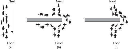
FIGURE 1.7 Illustrating the behavior of real ant movements.
1.4.1.2 The ACO Algorithm.
The main idea of ACO [50,51] is to model a problem as the search for a minimum cost path in a graph. Artificial ants as those walking on this graph, looking for cheaper paths. Each ant has a rather simple behavior capable of finding relatively costlier paths. Cheaper paths are found as the emergent result of the global cooperation among ants in the colony. The behavior of artificial ants is inspired from real ants: They lay pheromone trails (obviously in a mathematical form) on the graph edges and choose their path with respect to probabilities that depend on pheromone trails. These pheromone trails progressively decrease by evaporation. The basic idea of a real ant system is illustrated in Figure 1.7. In (a), the ants move in a straight line to the food. Part (b) illustrates the situation soon after an obstacle is inserted between the nest and the food. To avoid the obstacle, initially each ant chooses to turn left or right at random. Let us assume that ants move at the same speed depositing pheromone in the trail uniformly. However, the ants that, by chance, choose to turn left will reach the food sooner, whereas the ants that go around the obstacle turning right will follow a longer path, and so will take a longer time to circumvent the obstacle. As a result, pheromone accumulates faster in the shorter path around the obstacle. Since ants prefer to follow trails with larger amounts of pheromone, eventually all the ants converge to the shorter path around the obstacle, as shown in (c).
In addition, artificial ants have some extra features not seen in their counterpart in real ants. In particular, they live in a discrete world (a graph) and their moves consist of transitions from nodes to nodes. Pheromone placed on the edges acts like a distributed long-term memory. The memory, instead of being stored locally within individual ants, remains distributed on the edges of the graph. This indirectly provides a means of communication among the ants called stigmergy [50]. In most cases, pheromone trails are updated only after having constructed a complete path and not during the walk, and the amount of pheromone deposited is usually a function of the quality of the path. Finally, the probability for an artificial ant to choose an edge not only depends on pheromones deposited on that edge in the past, but also on some problem dependent local heuristic functions.
1.4.2 Type-2 Fuzzy Sets
The idea of types-2 fuzzy sets emerged from a 1975 paper by Zadeh [52], where he tried to address a typical problem with type-1 fuzzy sets that the membership function of type-1 fuzzy sets has no uncertainty associated with it. Thus this sometimes contradicts the word fuzzy, since that word has the connotation of lots of uncertainty. Type-2 fuzzy sets [53–55] are special kinds of fuzzy sets, the membership grades of which are themselves fuzzy (i.e., they incorporate a blurring of the type-1 membership function). The idea of type-2 fuzzy sets emerged from a 1975 paper by Zadeh [53], where he tried to address a typical problem with type-1 fuzzy sets that the membership function of a type-1 fuzzy set has no uncertainty associated with it. Thus this finding sometimes contradicts the word fuzzy, since that word has the connotation of lots of uncertainty. Now, in type-2 fuzzy sets, there is no longer a single value for the membership function for any input measurement or x value, but there are a few. This fact has been illustrated in Figure 1.8.
FIGURE 1.8 Illustrating the membership grades in (a) type-1 and (b) type-2 fuzzy sets.

In order to symbolically distinguish between a type-1 fuzzy set and a type-2 fuzzy set, researchers use a tilde symbol over the symbol for the latter fuzzy set; so, if A denotes a type-1 fuzzy set, à may denote the comparable type-2 fuzzy set. The distinguishing feature of à versus A is the membership function values of à are blurred, (i.e., they are no longer a single number from 0 to 1), but are instead a continuous range of values between 0 and 1, say [a, b]. We can either assign the same weighting or a variable weighting to the interval of membership function values [a, b]. When the former is done, the resulting type-2 fuzzy set is called either an interval type-2 fuzzy set or an interval valued fuzzy set (although different names may be used, they are the same fuzzy set). When the latter is done, the resulting type-2 fuzzy set is called a general type-2 fuzzy set (to distinguish it from the special interval type-2 fuzzy set).
The membership function of a general type-2 fuzzy set, Ã, is three-dimensional (3D) and the third dimension represents the value of the membership function at each point on its two-dimensional (2D) domain that is called its footprint of uncertainty (FOU). It is illustrated in Figure 1.9. For an interval type-2 fuzzy set that 3D value is the same (e.g., 1) everywhere, which means that no new information is contained in the third dimension of an interval type-2 fuzzy set. So, for such a set, the third dimension is ignored, and only the FOU is used to describe it. It is for this reason that an interval type-2 fuzzy set is sometimes called a first-order uncertainty fuzzy set model, whereas a general type-2 fuzzy set (with its useful third dimension) is sometimes referred to as a second-order uncertainty fuzzy set model.
FIGURE 1.9 Illustrating the 3D membership of a general type-2 fuzzy set. A cross section of one slice of the third dimension is shown. This cross section, as well as all others, sits on the FOU.

1.4.3 Rough Set Theory
Introduced by Pawlak [56,57] in the 1980s, rough set theory constitutes a sound basis for discovering patterns in hidden data and thus have extensive applications in data mining in distributed systems. It has recently emerged as a major mathematical tool for managing uncertainty that arises from granularity in the domain of discourse (i.e., from the indiscernibility between objects in a set).
Rough sets can be considered sets with fuzzy boundaries: Sets that cannot be precisely characterized using the available set of attributes. The basic concept of the rough set theory (RST) is the notion of approximation space, which is an ordered pair A=(U, R), where
U: Nonempty set of objects, called universe.
R: Equivalence relation on U, called indiscernibility relation. If x, y ε U and xRy then x and y are indistinguishable in A.
Each equivalence class induced by R, (i.e., each element of the quotient set ![]() = U/R, is called an elementary set in A. An approximation space can be alternatively noted by A = (U,
= U/R, is called an elementary set in A. An approximation space can be alternatively noted by A = (U,![]() ). It is assumed that the empty set is also elementary for every approximation space A. A definable set in A is any finite union of elementary sets in A. For x ε U let [x]R denote the equivalence class of R, containing x. For each X ⊆ U, X is characterized in A by a pair of sets: its lower and upper approximation in A, defined respectively as
). It is assumed that the empty set is also elementary for every approximation space A. A definable set in A is any finite union of elementary sets in A. For x ε U let [x]R denote the equivalence class of R, containing x. For each X ⊆ U, X is characterized in A by a pair of sets: its lower and upper approximation in A, defined respectively as
A rough set in A is the family of all subsets of U having the same lower and upper approximations. Figure 1.10 illustrates rough boundaries Alow(X) [the lower approximation and Aupp(X)] the upper approximation of a given point set X.
FIGURE 1.10 The rough boundaries Alow(X) [the lower approximation and Aupp(X)] the upper approximation of a given point set X⊆ U-the universe of discourse.

Many different problems can be addressed by RST. During the last few years, this formalism has been approached as a tool used in connection with many different areas of research. There have been investigations of the relations between RST and the Dempster–Shafer theory and between rough sets and fuzzy sets. The RST has also provided the necessary formalism and ideas for the development of some propositional machine learning systems. It has also been used for, among many others, knowledge representation; data mining; dealing with imperfect data; reducing knowledge representation, and for analyzing attribute dependencies. The notions of rough relations and functions are based on RST and can be applied as a theoretical basis for rough controllers, among others.
1.4.4 Granular Computing
The philosophy of rough set analysis is general enough to be applicable to many problem-solving tasks. It, in fact, has a major influence on an emerging field of study known as granular computing (GrC) [58–60]. The theory of rough sets and the theory of granularity offer artificial intelligence perspectives on granular computing. Specifically, granular computing can be viewed as a study of human-inspired problem solving and information processing. Granular computing concerns the processing of complex information entities called information granules, which arise in the process of data abstraction and derivation of knowledge from information. Generally speaking, information granules are collections of entities that usually originate at the numeric level and are arranged together due to their similarity, functional or physical adjacency, indistinguishability, coherency, or the like.
Currently, granular computing is more a theoretical perspective than a coherent set of methods or principles. As a theoretical perspective, it encourages an approach to data that recognizes and exploits the knowledge present in data at various levels of resolution or scales. In this sense, it encompasses all methods that provide flexibility and adaptability in the resolution at which knowledge or information is extracted and represented.
1.4.5 Artificial Immune Systems
The artificial immune systems (AIS) [61,62] have appeared as a new computational approach for the CI community. Like other biologically inspired techniques, it tries to extract ideas from a natural system, in particular the vertebrate immune system, in order to develop computational tools for solving engineering problems. The pioneering task of AIS is to detect and eliminate non-self materials, called “antigens” (e.g., virus cells or cancer cells). The artificial immune system also plays a great role to maintain its own system against dynamically changing environment. The immune system thus aims at providing a new methodology suitable for dynamics problems dealing with unknown–hostile environment.
In recent years, much attention has been focused on behavior-based AI for its proven robustness and flexibility in a dynamically changing environment. Artificial immune systems are one such behavior-based reactive system that aims at developing a decentralized consensus making mechanism, following the behavioral characteristics of biological immune system.
The basic components of the biological immune system are macrophages, antibodies, and lymphocytes, the last one being classified into two types: B- and T-lymphocytes [63], which are the cells stemming from the bone marrow. The human blood circulatory system contains roughly 107 distinct types of B-lymphocytes, each of which has a distinct molecular structure and produces Y-shaped [63] antibodies from its surface. Antibodies can recognize foreign substances, called antigens, that invade a living creature. Virus, cancer cells, and so on, are typical examples of antigens. To cope with a continuously changing environment, a living system possesses an enormous repertoire of antibodies in advance. The T-lymphocytes, on the other hand, are the cells maturing in the thymus, and are used to kill infected cells and regulate the generation of antibodies from B-lymphocytes as outside circuits of B-lymphocyte networks. It is interesting to note that an antibody recognizes an antigen by part of its structure called epitope. The portion of the antibody that has the recognizing capability of an antigen is called paratope. Usually, epitope is the key portion of the antigen, and paratope is the keyhole portion of the antibody. Recent study in immunology reveals that each type of antibody has its specific antigen determinant, called idiotope.
Jerne [63–65] proposed the idiotypic network hypothesisto explain the biological communication among different species of antibodies. According to the hypothesis, antibodies–lyphocytes are not isolated, but they communicate to each other among their variant species.
A simple model of the immune system can be put forward in the following way:
Let
αi(t) be the concentration of the ith antibody
mij be the affinity between antibody j and antibody i
mik be the affinity between antibody i and the detected antigen k
ki be the natural decay rate of antibody i
N and M, respectively, denote the number of antibodies that stimulate and suppress antibody i
The growth rate of antibody is given below:

The first and the second term on the right-hand side of Eq. (1.13), respectively, denote the stimulation and suppression by other antibodies, respectively. The third term denotes the stimulation from the antigen, and the fourth term represents the natural decay of the ith antibody. Equation (1.14) is a squashing function used to ensure the stability of the concentration.
1.4.6 Chaos Theory
In mathematics, chaos theory [66,67] describes the behavior of certain dynamical systems (i.e., systems whose states evolve with time) that may exhibit dynamics that are highly sensitive to initial conditions (popularly referred to as the butterfly effect). As a result of this sensitivity, which manifests itself as an exponential growth of perturbations in the initial conditions, the behavior of chaotic systems appears to be random. This happens even though these systems are deterministic, meaning that their future dynamics are fully defined by their initial conditions with no random elements involved. This behavior is known as deterministic chaos, or simply chaos. Chaos theory describes the behavior of certain nonlinear dynamical systems that under certain conditions exhibit a peculiar phenomenon known as chaos. One important characteristic of the chaotic systems is their sensitivity to initial conditions (popularly referred to as the butterfly effect). Because of this sensitivity, the behavior of these systems appears to be random, even though the dynamics is deterministic in the sense that it is well defined and contains no random parameters. Examples of such systems include the atmosphere, the solar system, plate tectonics, turbulent fluids, economics, and population growth.
Currently, fuzzy logic and chaos theory form two of the most intriguing and promising areas of mathematical research. Recently, fuzzy logic and chaos theory have merged to form a new discipline of knowledge, called fuzzy chaos theory [68,69]. The detailed implications of fuzzy chaotic models are beyond the scope of this chapter.
1.4.7 The Differential Evolution Algorithm
Differential evolution (DE) [70–72] is well known as a simple and efficient scheme for global optimization over continuous spaces. It has reportedly outperformed a few evolutionary algorithms (EAs) and other search heuristics like the PSO when tested over both benchmark and real-world problems. Differential evolution is a population-based global optimization algorithm that uses a floating-point (real-coded) representation. The ith individual (parameter vector or chromosome) of the population at generation (time) t is a D-dimensional vector containing a set of D optimization parameters:
Now, in each generation (or one iteration of the algorithm) to change the population members ![]() (say), a donor vector
(say), a donor vector ![]() is created. It is the method of creating this donor vector that distinguishes the various DE schemes. In one of the earliest variants of DE, now called the DE–rand–1 scheme, to create
is created. It is the method of creating this donor vector that distinguishes the various DE schemes. In one of the earliest variants of DE, now called the DE–rand–1 scheme, to create ![]() for each ith member, three other parameter vectors (say the r1, r2, and r3th vectors such that r1,r2,r3 ε [1,NP] and r1 ≠ r2 ≠ r3) are chosen at random from the current population. Next, the difference of any two of the three vectors is multiplied by a scalar number F and the scaled difference is added to the third one, hence we obtain the donor vector
for each ith member, three other parameter vectors (say the r1, r2, and r3th vectors such that r1,r2,r3 ε [1,NP] and r1 ≠ r2 ≠ r3) are chosen at random from the current population. Next, the difference of any two of the three vectors is multiplied by a scalar number F and the scaled difference is added to the third one, hence we obtain the donor vector ![]() . The process for the jth component of the ith vector may be expressed as,
. The process for the jth component of the ith vector may be expressed as,
Next, a crossover operation takes place to increase the potential diversity of the population. The DE family primarily uses two kinds of crossover schemes, namely, “exponential” and “binomial” [70]. To save space here, we briefly describe the binomial crossover, which is also employed by the modified DE algorithm. The binomial crossover is performed on each of the D variables whenever a randomly picked number between 0 and 1 is within the Cr value. In this case, the number of parameters inherited from the mutant has a (nearly) binomial distribution. Thus for each target vector ![]() , a trial vector
, a trial vector ![]() is created in the following fashion:
is created in the following fashion:
for j = 1, 2, …, D and randj (0, 1) ε [0,1] is the jth evaluation of a uniform random number generator. The Paramiter rn(i) ε [1,2,…,D] is a randomly chosen index that ensures ![]() gets at least one component from
gets at least one component from ![]() . To keep the population size constant over subsequent generations, the next step of the algorithm calls for “selection” in order to determine which one between the target and trial vector will survive in the next generation (i.e., at time t = t +1). If the trial vector yields a better value of the fitness function, it replaces its target vector in the next generation; otherwise the parent is retained in the population:
. To keep the population size constant over subsequent generations, the next step of the algorithm calls for “selection” in order to determine which one between the target and trial vector will survive in the next generation (i.e., at time t = t +1). If the trial vector yields a better value of the fitness function, it replaces its target vector in the next generation; otherwise the parent is retained in the population:
where f(.) is the function to be minimized.
The DE has successfully been applied to diverse domains of science and engineering (e.g., mechanical engineering design, signal processing, chemical engineering, machine intelligence, and pattern recognition, see [73]). It has been shown to perform better than the GA and PSO over several numerical benchmarks [74].
1.4.8 BFOA
In 2002, Passino and co-workers proposed the BFOA [75,76] based on the foraging theory of natural creatures that try to optimize (maximize) their energy intake per unit time spent for foraging, considering all the constraints presented by their own physiology (e.g., sensing and cognitive capabilities), and environment (e.g., density of prey, risks from predators, physical characteristics of the search space). Although BFOA has certain characteristics analogous to an evolutionary algorithm ([75], p. 63), it is not directly connected to Darwinian evolution and natural genetics, which formed the basis of the GA type algorithms in the early 1970s.
During foraging of the real bacteria, locomotion is achieved by a set of tensile flagella. Flagella help an Escherechia coli bacterium to tumble or swim, which are two basic operations performed by a bacterium at the time of foraging [70]. When they rotate the flagella in the clockwise direction, each flagellum pulls on the cell. That results in the moving of flagella independently and finally the bacterium tumbles with a lesser number of tumbling, whereas in a harmful place it tumbles frequently to find a nutrient gradient. Moving the flagella in the counterclockwise direction helps the bacterium to swim at a very fast rate. In the above-mentioned algorithm, the bacteria undergoes chemotaxis, where they like to move toward a nutrient gradient and avoid noxious environment. Generally, the bacteria move for a longer distance in a friendly environment. Figure 1.11 depicts how clockwise and counterclockwise movement of a bacterium take place in a nutrient solution.
FIGURE 1.11 Swim and tumble of a bacterium.

When they get sufficient food, they increased in length, and in the presence of a suitable temperature, they break in the middle to from an exact replica of themselves. This phenomenon inspired Passino to introduce an event of reproduction in BFOA. Due to the occurrence of sudden environmental changes or attack, the chemotactic progress may be destroyed and a group of bacteria may move to some other places or something else may be introduced in the swarm of concern. This constitutes the event of elimination dispersal in the real bacterial population, where all the bacteria in a region are killed or a group is dispersed into a new part of the environment.
Now, suppose that we want to find the minimum of J(θ), where ![]() is a p-dimensional vector of real numbers), and we do not have measurements or an analytical description of the gradient
is a p-dimensional vector of real numbers), and we do not have measurements or an analytical description of the gradient ![]() . The BFOA mimics the four principal mechanisms observed in a real bacterial system: chemotaxis, swarming, reproduction, and elimination dispersal to solve this nongradient optimization problem. Below, we introduce the formal notations used in BFOA literature, and then provide the complete pseudocode of the BFO algorithm.
. The BFOA mimics the four principal mechanisms observed in a real bacterial system: chemotaxis, swarming, reproduction, and elimination dispersal to solve this nongradient optimization problem. Below, we introduce the formal notations used in BFOA literature, and then provide the complete pseudocode of the BFO algorithm.
Let us define a chemotactic step to be a tumble followed by a tumble or a tumble followed by a run. Let j be the index for the chemotactic step. Let k be the index for the reproduction step. Let l be the index of the elimination-dispersal event. Also, let
p = Dimension of the search space
S = Total number of bacteria in the population
Nc = The number of chemotactic steps
Ns = The swimming length
Nre = The number of reproduction steps
Ned = The number of elimination-dispersal events
Ped = Elimination-dispersal probability
C (i) = The size of the step taken in the random direction specified by the tumble
Let ![]() represent the position of each member in the population of the S bacteria at the jth chemotactic step, kth reproduction step, and lth elimination-dispersal event. Here, let J(i,j,k,l) denote the cost at the location of the ith bacterium
represent the position of each member in the population of the S bacteria at the jth chemotactic step, kth reproduction step, and lth elimination-dispersal event. Here, let J(i,j,k,l) denote the cost at the location of the ith bacterium ![]() (sometimes we drop the indices and refer to the ith bacterium position as θi). Note: We will interchangeably refer to J as being a “cost” (using terminology from optimization theory) and as being a nutrient surface (in reference to the biological connections). For actual bacterial populations, S can be very large (e.g., =109), but p= 3. In our computer simulations, we will use much smaller population sizes and will keep the population size fixed. However, the BFOA, allows p>3 so that we can apply the method to higher dimensional optimization problems. Below we briefly describe the four prime steps in BFOA. We also provide a pseudocode of the complete algorithm.
(sometimes we drop the indices and refer to the ith bacterium position as θi). Note: We will interchangeably refer to J as being a “cost” (using terminology from optimization theory) and as being a nutrient surface (in reference to the biological connections). For actual bacterial populations, S can be very large (e.g., =109), but p= 3. In our computer simulations, we will use much smaller population sizes and will keep the population size fixed. However, the BFOA, allows p>3 so that we can apply the method to higher dimensional optimization problems. Below we briefly describe the four prime steps in BFOA. We also provide a pseudocode of the complete algorithm.
1. Chemotaxis. This process simulates the movement of an E. coli cell through swimming and tumbling via flagella. Suppose θi (j,k,l) represents ith bacterium at the jth chemotactic, kth reproductive, and lth elimination-dispersal step. The parameter C(i) is a scalar and indicates the size of the step taken in the random direction specified by the tumble (run length unit). Then in computational chemotaxis, the movement of the bacterium may be represented by
where Δ indicates a unit length vector in the random direction.
2. Swarming. An interesting group behavior has been observed for several motile species of bacteria including E. coli and Salmonella typhimurium, where stable spatiotemporal patterns (swarms) are formed in a semisolid nutrient medium. A group of E. coli cells arrange themselves in a traveling ring by moving up the nutrient gradient when placed amid a semisolid matrix with a single nutrient chemoeffecter. The cells when stimulated by a high level of succinate, release an attractant aspertate, which helps them to aggregate into groups and thus move as concentric patterns of swarms with high bacterial density. The cell-to-cell signaling in E. coli swarm may be represented by the following function:

where Jcc (θ,P(j,k,l)) is the objective function value to be added to the actual objective function (to be minimized) to present a time varying objective function. The coefficients dattractant, wattractant, hrepellant, and wrepellant control the strength of the cell-to-cell signaling. More specifically dattractant is the depth of the attractant released by the cell; wattractant is a measure of the width of the attractant signal (a quantification of the diffusion rate of the chemical); hrepellant = dattractant is the height of the repellant effect (a bacterium cell also repels a nearby cell in the sense that it consumes nearby nutrients and it is not physically possible to have two cells at the same location); and wrepellant is a measure of the width of the repellant. For a detailed discussion on the function Jcc, please see [70].
3. Reproduction. The least healthy bacteria eventually die while each of the healthier bacteria (those yielding lower value of the objective function) asexually split into two bacteria, which are then placed in the same location. This keeps the swarm size constant.
4. Elimination and Dispersal. To simulate this phenomenon in BFOA, some bacteria are liquidated at random with a very small probability while the new replacements are randomly initialized over the search space.
1.4.9 Bees Foraging Algorithm
Besides the gradually increasing popularity of BFOA, the current decade also witnessed the development of a family of computer algorithms mimicking the foraging strategies of honey bees. A colony of honey bees can extend itself over long distances (up to 14 km) and in multiple directions simultaneously to exploit a large number of food sources. A colony prospers by deploying its foragers to good fields. In principle, flower patches with plentiful amounts of nectar or pollen that can be collected with less effort should be visited by more bees, whereas patches with less nectar or pollen should receive fewer bees [77,78]. The foraging process begins in a colony by scout bees being sent to search for promising flower patches. Scout bees move randomly from one patch to another. During the harvesting season, a colony continues its exploration, keeping a percentage of the population as scout bees. When they return to the hive, those scout bees founding a patch that is rated above a certain quality threshold (measured as a combination of some constituents, e.g., sugar content) deposit their nectar or pollen and go to the “dance floor” to perform a dance known as the Waggle Dance [41]. The family of Artificial Bee Foraging algorithms try to mimic the above aspects of the foraging strategies employed by real bee colonies. The key members of the family and their applications to several different engineering optimization problems have been summarized in Table 1.2.
TABLE 1.2 A Summary of State-of-the-art Research Works on Bees Foraging Algorithm
Recently, Quijano et al. [94] modeled the social foraging behavior of honey bees for nectar, involving the environment representation, activities during bee expeditions (exploration and foraging), unloading nectar, dance strength decisions, explorer allocation, recruitment on the dance floor, and accounting for interactions with other hive functions [95]. They used the computational model of bee foraging to (1) solve a continuous optimization problem underlying resource allocation, and (2) provide novel strategies for multizone temperature control, an important industrial engineering application. They also established the global optimality of such algorithms for single or multiple hives theoretically on the resource allocation problem.
1.5 SUMMARY
This chapter introduced different fundamental components of CI, discussed their scope of possible synergism, and also focused on the most prominent recent topics emerging in the field. It is clear from the discussions that fuzzy logic is a fundamental tool for reasoning with approximate data and knowledge. Neural network plays a significant role in machine learning and GA has an extensive application in intelligent search and optimization problems. Belief networks are capable of propagating beliefs of an event node based on the probabilistic support of its cause and effect nodes in the causal tree–graph. The chapter also provided a list of possible synergism of two or more computational models that fall under the rubric of CI. It ends with a brief exposure to some very recently developed methodologies, which are gaining rapid importance in the realm of CI.
REFERENCES
1. A. M. Turing (1936), On Computable Numbers, with an Application to the Entscheidungs problem, Proc. London Math. Soc., 2, 42: 230–265.
2. Turing Machine: Available at http://www.turing.org.uk/turing/.
3. A. M. Turing (1950), Computing Machinery and Intelligence Available at http://abelard.org/turpap/turpap.htm.
4. A. M. Turing (1948), Machine Intelligence, in B. J. Copeland (Ed.), The Essential Turing: The ideas that gave birth to the computer age, Oxford University Press, Oxford, UK.
5. J. C. Bezdek (1994), What is Computational Intelligence? Computational Intelligence Imitating Life, J. M., Zurada, R. J. Marks, and C. J. Robinson (Eds.), IEEE Press, NY, pp. 1–12.
6. A. Konar (2005), Computational Intelligence, Principles, Techniques, and Applications, Springer-Verlag, Berlin, Heidelberg.
7. D. Poole, A. Mackworth, and R. Goebel (1998), Computational Intelligence—A Logical Approach, Oxford University Press, NY.
8. A. P. Engelbrecht (2007), Computational Intelligence: An Introduction, John Wiley & Sons, Inc., NY.
9. R. J., Marks (1993), Intelligence: Computational versus Artificial, IEEE Trans. Neural Networks, 4: 737–739.
10. C. G. Langton (Ed.) (1989), Artificial Life, Vol. 6, Addison-Wesley, Reading, MA.
11. W. Pedrycz (1996), Fuzzy Sets Engineering, CRC Press, Boca Raton, FL, pp. 73–106.
12. W. Pedrycz and F. Gomide (1998), An Introduction to Fuzzy Sets: Analysis and Design, MIT Press, MA.
13. S. Haykin (1999), Neural Networks: A Comprehensive Foundation, Prentice-Hall, NJ.
14. Li. M. Fu (1994), Neural Networks in Computer Intelligence, McGraw-Hill, NY.
15. J., Hertz, A. Krogn, and G. R. Palmer (1990), Introduction to the Theory of Neural Computation, Addison-Wesley, Reading, MA.
16. R. J. Schalkoff (1997), Artificial Neural Networks, McGraw-Hill, NY.
17. S. Kumar (2007), Neural Networks—A Classroom Approach, Tata, McGraw-Hill, India.
18. C. M. Bishop (1995), Neural Networks for Pattern Recognition, Oxford University Press.
19. T. Kohonen (1988), Self-Organization and Associative Memory, Springer-Verlag, NY.
20. Zadeh, L. A. (1965), Fuzzy Sets, Information and Control, Vol. 8: pp. 338–353.
21. G. J. Klir and B. Yuan (1995), Sets and Fuzzy Logic: Theory and Applications, Prentice-Hall, NJ.
22. B. Kosko (1991), Neural Networks and Fuzzy Systems: A Dynamical Systems Approach to Machine Intelligence, Prentice-Hall, Englewood Cliffs, NJ.
23. T. J. Ross (1995), Fuzzy Logic with Engineering Applications, McGraw-Hill, NY.
24. H. J. Zimmerman (1996), Fuzzy Set Theory and Its Applications, Kluwer Academic, Dordrecht, The Netherlands, pp. 131–162.
25. A. Abraham (2001), Neuro-Fuzzy Systems: State-of-the-Art Modeling Techniques, Connectionist Models of Neurons, Learning Processes, and Artificial Intelligence, Lecture Notes in Computer Science. Mira J. and Prieto A. (Eds.), Vol. 2084, Springer-Verlag Germany, pp. 269–276.
26. T. Back, D. B. Fogel, and Z. Michalewicz (Eds.) (1997), Handbook of Evolutionary Computation, Oxford University Press.
27. D. B. Fogel (1995), Evolutionary Computation: Toward a New Philosophy of Machine Intelligence, IEEE Press, Piscataway, NJ.
28. L. J., Fogel, A. J. Owens, and M. J. Walsh (1966), Artificial Intelligence through Simulated Evolution, John Wiley & Sons, NY.
29. J. H. Holland (1975), Adaptation in Natural and Artificial Systems, University of Michigan Press, Ann Arbor, MI.
30. I. Rechenberg (1973), Evolutionsstrategie—Optimierung Technischer Systeme nach Prinzipien der Biologischen Evolution (Ph.D. thesis, 1971), Reprinted by Fromman-Holzboog.
31. H.-P. Schwefel (1974), Numerische Optimierung von Computer-Modellen (Ph.D. thesis). Reprinted by Birkhäuser (1977).
32. J. R. Koza (1992), Genetic Programming: On the programming of Computers by Means of Natural Selection, MIT Press, Cambridge, MA.
33. E. Bonabeau, M. Dorigo, and G. Theraulaz (1999), Swarm Intelligence: From Natural to Artificial Systems, Oxford University Press Inc.
34. T. M. Martinetz and K. J. Schulten (1991), A neural-gas network learns topologies, T. Kohonen, K. Mäkisara, O. Simula, and J. Kangas (Eds.), Artificial Neural Networks, North-Holland, Amsterdam, The Netherlands, pp. 397–402.
35. Z. Kobti, R. Reynolds, and T. Kohler (2003), A multi-agent simulation using cultural algorithms: The effect of culture on the resilience of social systems, IEEE Congress on Evolutionary Computation December 5–12, 2003, Canberra, Australia.
36. K. S. Lee and Z. W. Geem (2005), A new meta-heuristic algorithm for continuous engineering optimization: harmony search theory and practice, Computer Methods in Applied Mechanics and Engineering, Vol. 194, No. 36–38, pp. 3902–3933.
37. D. Dasgupta (Ed.) (1999), Artificial Immune Systems and Their Applications, Springer-Verlag, Inc. Berlin.
38. J. Wojtusiak and R. S. Michalski (2006), The LEM3 Implementation of learnable evolution model and Its testing on complex function optimization problems, Proceedings of Genetic and Evolutionary Computation Conference, GECCO 2006, Seattle, WA.
39. J. Pearl (1997), Probabilistic Reasoning in Intelligent Systems: Networks of Plausible Inference, Morgan Kaufmann Publishers.
40. J. Pearl (1987), Distributed revision of composite beliefs, Artificial Intelligence, Vol. 33, pp. 173–213.
41. J. Pearl (1986), {Fusion, propagation and structuring in belief networks, Artificial Intelligence,} Vol. 29, pp. 241–288.
42. A. Abraham (2002), Intelligent Systems: Architectures and Perspectives, Recent Advances in Intelligent Paradigms and Applications, A. Abraham, L. Jain, and J. Kacprzyk (Eds.), Studies in Fuzziness and Soft Computing, Springer-Verlag Germany, Chapter 1, pp. 1–35.
43. G. Beni and U. Wang (1989), Swarm intelligence in cellular robotic systems, NATO Advanced Workshop on Robots and Biological Systems, Il Ciocco, Italy.
44. I. D. Couzin, J. Krause, R. James, G. D. Ruxton, and N. R. Franks (2002), Collective Memory and Spatial Sorting in Animal Groups, J. Theor. Biol., 218: 1–11.
45. J. Krause and G. D. Ruxton (2002), Living in Groups, Oxford University Press, Oxford, UK.
46. B. L. Partridge and T. J. Pitcher (1980), The sensory basis of fish schools: relative role of lateral line and vision. J. Compar. Physiol., 135: 315–325.
47. B. L. Partridge (1982), The structure and function of fish schools. Sci. Am., 245: 90–99.
48. M. M. Milonas (1994), Swarms, phase transitions, and collective intelligence, Artificial Life III, Langton CG (Ed.), Addison-Wesley, Reading, MA.
49. J. Kennedy, R. Eberhart, and Y. Shi (2001), Swarm Intelligence, Morgan Kaufmann Academic Press.
50. M. Dorigo, V. Maniezzo, and A. Colorni (1996), The ant system: Optimization by a colony of cooperating agents, IEEE Trans. Systems Man and Cybernetics Part B, 26.
51. M. Dorigo and L. M. Gambardella (1997), Ant colony system: A cooperative learning approach to the traveling salesman problem, IEEE Trans. Evolutionary Computing, 1: 53–66.
52. L. A. Zadeh (1975), The Concept of a Linguistic Variable and Its Application to Approximate Reasoning–1, Information Sci., 8: 199–249.
53. J. M. Mendel and R. I. John (2002), Type-2 Fuzzy Sets Made Simple, IEEE Trans. Fuzzy Systems, 10: 117–127.
54. O. Castillo and P. Melin (2008), Type-2 Fuzzy Logic Theory and Applications, Springer-Verlag, Berlin.
55. J. M. Mendel, R. L. John, and F. Liu (2006), Interval type-2 fuzzy logic systems made simple, IEEE Trans. Fuzzy Systems, 14: 808–821.
56. Z. Pawlak, S. K. M. Wong, and W. Ziarko (1988), Rough sets: Probabilistic versus deterministic approach, Inter. J. Man-Machine Studies 29: 81–95.
57. Z. Pawlak (1991), Rough Sets: Theoretical Aspects of Reasoning About Data, Dordrecht: Kluwer Academic Publishing.
58. A. Bargiela and W. Pedrycz (2003), Granular Computing. An introduction, Kluwer Academic Publishers.
59. W. Pedrycz, A. Skowron, and V. Kreinovich (Eds.) (2008), Handbook of Granular Computing, John Wiley & Sons, Inc., NY.
60. R. Bello, R. Falcón, W. Pedrycz, and J. Kacprzyk (Eds.) (2008), Granular Computing: At the Junction of Rough Sets and Fuzzy Sets, Springer-Verlag, NY.
61. D. Dasgupta (Ed.) (1999), Artificial Immune Systems and Their Applications, Springer-Verlag, Inc., Berlin.
62. J. O. Kephart (1994), A biologically inspired immune system for computers, Proceedings of Artificial Life IV: The Fourth International Workshop on the Synthesis and Simlation of Living Systems, MIT Press, MA, pp. 130–139.
63. N. K. Jerne (1973), The immune systems, Sci. Am., 229(1): 52–60.
64. N. K. Jerne (1983), The generative grammar of the immune system, EMBO J., 4(4): 847–852.
65. N. K. Jerne (1984), Idiotypic networks and other pre-conceived ideas, Immunolog. Rev., 79: 5–24.
66. R. L. Devaney (2003), An Introduction to Chaotic Dynamical Systems, 2nd ed,. Westview Press.
67. E. Ott (2002), Chaos in Dynamical Systems, Cambridge University Press, NY.
68. J. J. Buckley (1991), Fuzzy dynamical systems, Proceedings of IFSA’91, Brussels, Belgium, pp. 16–20.
69. P. Grim (1993), Self-Reference and Chaos in Fuzzy Logic, IEEE Trans. Fuzzy Systems, 1(4): 237–253.
70. R. Storn, K. V. Price, and J. Lampinen (2005), Differential Evolution—A Practical Approach to Global Optimization, Springer, Berlin.
71. U. K. Chakraborty (Ed.) (2008), Advances in Differential Evolution, Springer-Verlag, Heidelberg.
72. V. Feoktistov (2006), Differential Evolution—In Search of Solutions, Springer, Heidelberg.
73. J. Lampinen (1999), A bibliography of differential evolution algorithm, Technical Report. Lappeenranta University of Technology, Department of Information Technology, Laboratory of Information Processing, 1999. Available at http://www.lut.fi/∼jlampine/ debiblio.htm.
74. J. Vesterström and R. Thomson (2004), A comparative study of differential evolution, particle swarm optimization, and evolutionary algorithms on numerical benchmark problems, Proceedings of the Sixth Congress on Evolutionary Computation (CEC-2004), IEEE Press.
75. K. M. Passino (2002), Biomimicry of bacterial foraging for distributed optimization and control, IEEE Control Systems Mag., 52–67.
76. Y. Liu and K. M. Passino (2002), Biomimicry of social foraging bacteria for distributed optimization: models, principles, and emergent behaviors, J. Optimization Theory App., 115(3): 603–628.
77. K. V. Frisch (1976), Bees: Their Vision, Chemical Senses and Language, (Revised edition) Cornell University Press, Ithaca, NY.
78. S. Camazine, J. Deneubourg, N. R. Franks, J. Sneyd, G. Theraula, and E. Bonabeau (2003), Self-Organization in Biological Systems, Princeton University Press, Princeton, NY.
79. Y. Yonezawa and T. Kikuchi (1996), Ecological Algorithm for Optimal Ordering Used by Collective Honey Bee Behavior, 7th International Symposium on Micro Machine and Human Science, 249–256.
80. T. D. Seeley and S. C. Buhrman (1999), Group decision making in swarms of honey bees, Behav. Ecol. Sociobiol., 45: 19–31.
81. T. Schmickl, R. Thenius, and K. Crailsheim (2005), Simulating swarm intelligence in honey bees: foraging in differently fluctuating environments, Genetic and Evolutionary Computation Conference (GECCO 2005), Washington, DC, pp. 273–274.
82. N. P. P. M. Lemmens (2006), To bee or not to bee: a comparative study in swarm intelligence, Master thesis, Maastricht University, Maastricht ICT Competence Centre, Institute for Knowledge and Agent Technology, Maastricht, Netherlands, 2006.
83. T. Sato and M. Hagiwara (1997), Bee system: finding solution by a concentrated search, Proceedings of the IEEE International Conference on Systems, Man, and Cybernetics, Vol. 4(C), pp. 3954–3959.
84. D. Karaboga (2005), An idea based on honey bee swarm for numerical optimization, Technical Report-TR06, Erciyes University, Engineering Faculty, Computer Engineering Department, Turkey.
85. X. S. Yang (2005), Engineering optimizations via nature-inspired virtual bee algorithms, IWINAC 2005, LNCS 3562, J. M. Yang and J. R. Alvarez (Eds.), Springer-Verlag, Berlin Heidelberg, pp. 317–323.
86. D. T. Pham, E. Kog, A. Ghanbarzadeh, S. Otri, S. Rahim, and M. Zaidi (2006), The bees algorithm—a novel tool for complex optimization problems, IPROMS 2006 Proceeding 2nd International Virtual Conference on Intelligent Production Machines and Systems, Elsevier, Oxford, UK.
87. P. Lucic and D. Teodorovic (2001), Bee system: modeling combinatorial optimization transportation engineering problems by swarm intelligence, Preprints of the TRISTAN IV Triennial Symposium on Transportation Analysis, Sao Miguel, Azores Islands, pp. 441–445.
88. P. Luckic and D. Teodorovic (2002), Transportation modeling: an artificial life approach, ICTAI’02 14th IEEE International Conference on Tools with Artificial Intelligence, pp. 216–223.
89. D. Teodorovic and M. Dell’Orco (2005), Bee colony optimization—a cooperative learning approach to complex transportation problems, Advanced OR and AI Methods in Transportation, pp. 51–60.
90. S. Nakrani and C. Tovey (2003), On honey bees and dynamic allocation in an internet server colony, Proceedings of 2nd International Workshop on the Mathematics and Algorithms of Social Insects, Atlanta, GA.
91. H. F. Wedde, M. Farooq, and Y. Zhang (2004), BeeHive: An Efficient Fault-Tolerant Routing Algorithm Inspired by Honey Bee Behavior, Ant Colony, Optimization and Swarm Intelligence, M. Dorigo (Ed.), Lecture Notes in Computer Science 3172, Springer, Berlin, pp. 83–94.
92. H. Drias, S. Sadeg, and S. Yahi (2005), Cooperative bees swarm for solving the maximum weighted satisfiability problem, IWAAN International Work Conference on Artificial and Natural Neural Networks, Barcelona, Spain, pp. 318–325.
93. D. T. Pham, S. Otri, A. Ghanbarzadeh, and E. Kog (2006), Application of the bees algorithm to the training of learning vector quantization networks for control chart pattern recognition, ICTTA’06 Information and Communication Technologies, pp. 1624–1629.
94. N. Quijano, B. W. Andrews, and K. M. Passino (2006), Foraging theory for multizone temperature control, IEEE Computational Intelligence Mag., 1(4): 18–27.
95. N. Quijano and K. M. Passino (2007), The ideal free distribution: theory and engineering application, IEEE Transactions Systems, Man, Cybernetics Part B, 37(1): 154–165.