5

PLANNING AND CONTROL OF MANUFACTURING COSTS: MANUFACTURING EXPENSES

NATURE OF MANUFACTURING EXPENSES

The indirect manufacturing expenses or overhead costs of a manufacturing operation have increased significantly as business has become more complex, and the utilization of more sophisticated machinery and equipment is more prevalent. As the investment in computer-controlled machinery has increased, improving productivity and reducing direct labor hours, the control of depreciation expense, power costs, machinery repairs and maintenance, and similar items has received a greater emphasis by management.

Manufacturing overhead has several distinguishing characteristics as compared with the direct manufacturing costs of material and labor. It includes a wide variety of expenses, such as depreciation, property taxes, insurance, fringe benefit costs, indirect labor, supplies, power and other utilities, clerical costs, maintenance and repairs, and other costs that cannot be directly identified to a product, process, or job. These types of costs behave differently from direct costs, as the volume of production varies. Some will fluctuate proportionately as production increases or decreases, and some will remain constant or fixed and will not be sensitive to the change in the number of units produced. Some costs are semivariable and for a particular volume level are fixed; however, they may vary with volume but less proportionately and probably can be segregated into their fixed and variable components.

The control of overhead costs rests with many individuals involved in the manufacturing process. Certain costs such as repairs and maintenance are controlled by the head of the maintenance department. Manufacturing supplies may be controlled by each department head who uses the supplies in carrying out his function. Other costs may be decided by management and assigned to a particular manager for control—for example, depreciation, taxes, insurance. Accounting planning and control of manufacturing indirect expenses is diverse and a challenging opportunity for the controller.

RESPONSIBILITY FOR PLANNING AND CONTROL OF MANUFACTURING EXPENSES

Responsibility for the planning and control of manufacturing expenses is clearly that of the manufacturing or production executive. However, this executive will be working through a financial information system largely designed by the chief accounting official or his staff—although there should be full participation by the production staff on many aspects of the system development.

In formulating the expense account structure under which expenses will be planned and actual expenses matched against the budget or other standards, the controller should heed these common sense suggestions to make the reports more useful to the manufacturing executive:

• The budget (or other standard) should be based on technical data that are sound from a manufacturing viewpoint.

  Among other things, this will call for cooperation with the industrial engineers or process engineers who will supply the technical data required in developing the budget and/or standards. As manufacturing processes change, the standards must change. Adoption of just-in-time (JIT) techniques may require, for example, a different alignment of cost centers. Further, with the increased use of robots or other types of mechanization, direct labor will play a less important role, while manufacturing expense (through higher depreciation charges, perhaps more indirect labor, higher repairs and maintenance, and power) will become relatively more significant.

• The manufacturing department supervisors, who will do the actual planning and control of expenses, must be given the opportunity to fully understand the system, including the manner in which the budget expense structure is developed, and to generally concur in the fairness of the system.
• The account classifications must be practical, the cost departments should follow the manufacturing organization structure (responsibility accounting and reporting), and the allocation methods must permit the proper valuation of inventories (usually under general accepted accounting principles), as well as proper control of expense.
• The manufacturing costs must be allocated as accurately as possible, so the manufacturing executive can determine the expense of various products and processes. This topic is covered in more detail later in this chapter, under activity-based costing.

Also, industrial engineers will provide the technical data required for the development of standards, such as manpower needs, power requirements, expected downtime, and maintenance requirements. Finally, if an activity-based costing (ABC) system is in place, then the manufacturing executive should work with the controller to develop information collection procedures for resource drivers.

APPROACH IN CONTROL OF MANUFACTURING EXPENSES

The diverse types of expenses in overhead and the divided responsibility may contribute to the incurrence of excessive costs. Furthermore, the fact that many cost elements seem to be quite small and insignificant in terms of consumption or cost per unit often encourages neglect of proper control. For example, it is natural to increase clerical help as required when volume increases to higher levels, but there is a reluctance and usually a delay from a timing viewpoint in eliminating such help when no longer needed. The reduced requirement must be forecasted and anticipated and appropriate actions taken in a timely manner. There are numerous expenses of small unit-cost items that may be insignificant but in the aggregate can make the company less competitive. Some examples are excessive labor hours for maintenance, use of special forms or supplies when standard items would be sufficient, personal use of supplies, and indiscriminate use of communication and reproduction facilities. All types of overhead expenses must be evaluated and controls established to achieve cost reduction wherever possible.

Although these factors may complicate somewhat the control of manufacturing overhead, the basic approach to this control is fundamentally the same as that applying to direct costs: the setting of budgets or standards, the measurement of actual performance against these standards, and the taking of corrective action when those responsible for meeting budgets or standards repeatedly fail to reach the goal. Standards may change at different volume levels; or stated in other terms, they must have sufficient flexibility to adjust to the level of operations under which the supervisor is working. To this extent the setting and application of overhead standards may differ from the procedure used in the control of direct material and direct labor. The degree of refinement and extent of application will vary with the cost involved. The controller should make every attempt to apply fair and meaningful standards, not thinking that little is needed or that nothing can be accomplished.

Also, the controller can use ABC to assign costs to products (or other entities, such as production departments or customers). This approach is better than the traditional method of assigning a uniform overhead rate to all production, since it assigns overhead costs to specific products based on their use of various activities, resulting in more accurate product costs.

PROPER DEPARTMENTALIZATION OF EXPENSES

One of the most essential requirements for either adequate cost control or accurate cost determination is the proper classification of accounts. Control must be exercised at the source, and since costs are controlled by individuals, the primary classification of accounts must be by individual responsibility—“responsibility accounting.” This generally requires a breakdown of expenses by factory departments that may be either productive departments or service departments, such as maintenance, power, or tool crib. Sometimes, however, it becomes necessary to divide the expense classification more finely to secure a proper control or costing of products—to determine actual expenses and expense standards by cost center. This decision about the degree of refinement will depend largely on whether improved product costs result or whether better expense control can be achieved.

A cost center, which is ordinarily the most minute division of costs, is determined on one of the following bases:

• One or more similar or identical machines
• The performance of a single operation or group of similar or related operations in the manufacturing process

The separation of operations or functions is essential because a foreman may have more than one type of machine or operation in his department—all of which affect costs. One product may require the use of expensive machinery in a department, and another may need only some simple hand operations. The segregation by cost center will reveal this cost difference. Different overhead rates are needed to reflect differences in services or machines required.

If the controller chooses to install an ABC system, a very different kind of cost breakdown will be required. The ABC method collects costs by activities, rather than by department; for example, information might be collected about the costs associated with engineering change orders, rather than the cost of the entire engineering department. If management decides that it wants both ABC and departmental cost information, then the controller must record the information twice—once by department and again by activity.

VARIATIONS IN COST BASED ON FIXED AND VARIABLE COSTS¹

One factor that can cause costs to vary is that they contain both variable and fixed elements. The cost of most products is itemized in a bill of materials (BOM) that itemizes all the components that are assembled into it. An example of a bill of materials for a desk light is shown in Exhibit 5.1. Each of the line items in this BOM are variable costs, for each one will be incurred only if a desk light is created—that is, the costs vary directly with unit volume.

In its current format, the BOM is very simple; we see a quantity for each component, a cost per component, and a total cost for each component that is derived by multiplying the number of units by the cost per unit. The only line item in this BOM that does not include a cost per unit or number of units is the overhead cost, which is situated near the bottom. This line item represents a variety of costs that are being allocated to each desk lamp produced. The costs included in this line item represent the fixed costs associated with lamp production. For example, there may be a legal cost associated with a patent that covers some feature of the desk lamp, the cost of a production supervisor who runs the desk lamp assembly line, a buyer who purchases components, the depreciation on any equipment used in the production process—the list of possible costs is lengthy. The key factor that brings together these fixed costs is that they are associated with the production of desk lamps, but they do not vary directly with the production of each incremental lamp. For example, if one more desk lamp is produced, there will be no corresponding increase in the legal fees needed to apply for or protect the patent that applies to the lamp.

This splitting of costs between variable and fixed costs can occupy the extremes of entirely fixed costs or entirely variable ones, with the most likely case being a mix of the two. For example, a software company that downloads its products over the Internet has entirely fixed costs; it incurs substantial costs to develop the software and set up a web site for downloading purposes, but then incurs zero costs when a customer downloads the software from the web site (though even in this case, there will be a small credit card processing fee charged on each transaction). Alternatively, a custom programming company will charge customers directly for every hour of time its programmers spend on software development, so that all programming costs are variable (though any administrative costs still will be fixed). To use a variation on the software example, a software developer that sells its products by storing the information on CDs or diskettes, printing instruction manuals, and mailing the resulting packages to customers will incur variable costs associated with the mailed packages, and fixed costs associated with the initial software development. All three variations on the variable-fixed cost mix are shown in Exhibit 5.2. In the exhibit, the first graph shows a straight horizontal line, indicating that there is no incremental cost associated with each additional unit sold. The second graph shows a steeply sloped line that begins at the X-Y intercept, which indicates that all costs are incurred as the result of incremental unit increases in sales. Finally, the third graph shows the sloped line beginning partway up the left side of the graph, which indicates that some (fixed) costs will be incurred even if no sales occur.

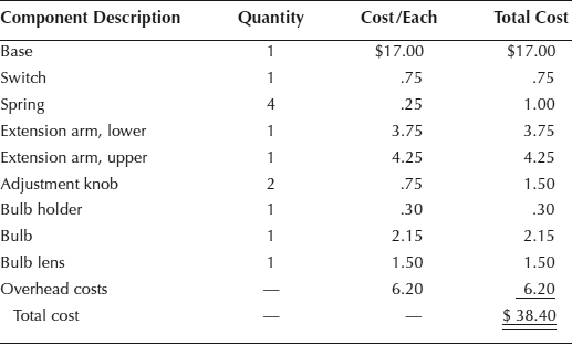
EXHIBIT 5.1 BILL OF MATERIALS

To return to the BOM listed earlier in Exhibit 5.1, the format does a good job of itemizing the variable costs associated with the desk lamp, but a poor one of describing the fixed costs associated with the product; there is only a single line item for $6.20 that does not indicate what costs are included in the overhead charge, nor how it was calculated. In most cases, the number was derived by summarizing all overhead into a single massive overhead cost pool for the entire production facility, which is then allocated out to the various products based on the proportion of direct labor that was charged to each product. However, many of the costs in the overhead pool may not be related in any way to the production of desk lamps, nor may the use of direct labor hours be an appropriate way in which to allocate the fixed costs.

This is a key area in which the costing information provided by controllers can result in incorrect management decisions of various kinds. For example, if the purpose of a costing inquiry by management is to add a standard margin to a cost and use the result as a product's new price, then the addition of a fixed cost that includes nonrelevant costs will result in a price that is too high. Similarly, using the same information but without any fixed cost may result in a price that is too low to ever cover all related fixed costs unless enormous sales volumes can be achieved. One of the best ways to avoid this problem with the proper reporting of fixed costs is to split the variable and fixed cost portions of a product's cost into two separate pieces, and then report them as two separate line items to the person requesting the information. The variable cost element is reported as the cost per unit, while the fixed cost element is reported as the entire fixed cost pool, as well as the assumed number of units over which the cost pool is being spread. To use the desk lamp example, the report could look like this:

We do not know the precise use to which our costing information will be put by the person requesting the preceding information, so we are giving her the key details regarding the fixed and variable cost elements of the desk lamp, from which she can make better decisions than would be the case if she received only the total cost of the desk lamp. This approach yields better management information, but, as we will see in the following sections, there are many other issues that can also impact a product's cost and that a controller should be aware of before issuing costing information to the rest of the organization.

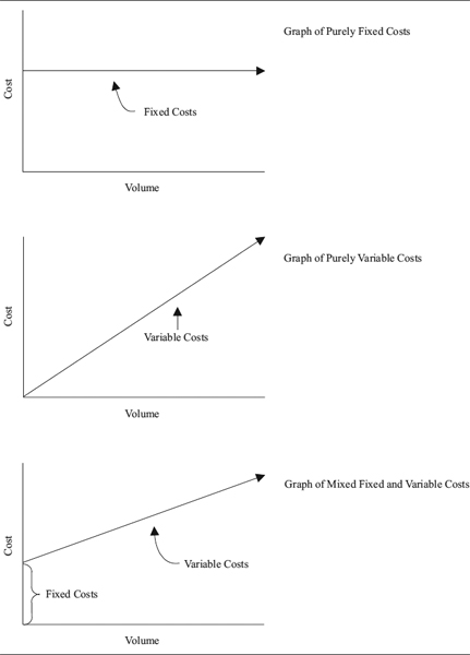
EXHIBIT 5.2 GRAPHS OF FIXED COSTS, VARIABLE COSTS, AND MIXED COSTS

VARIATIONS IN COST BASED ON DIRECT LABOR

One of the larger variable costs noted in a product's bill of materials is direct labor. This is the cost of all labor that is directly associated with the manufacture of a product. For example, it includes the cost of an assembly person who creates a product, or the machine operator whose equipment stamps out the parts that are later used in a product. However, it does not include a wide range of supporting activities, such as machine maintenance, janitorial services, production scheduling, or management, for these activities cannot be quite so obviously associated with a particular product. Consequently, direct labor is itemized separately on the BOM (as noted in Exhibit 5.3), while all other indirect labor elements are lumped into the fixed cost line item. In the exhibit, we have now switched from just one type of unit-based cost, as was noted in Exhibit 5.1, to two types of costs; one is still based on a cost per unit, but now we have included direct labor, which is based on a cost per hour. Accordingly, there is now a “unit of measure” column in the BOM that identifies each type of cost. The two types of direct labor itemized in the BOM are listed as a cost per hour, along with the fraction of an hour that is required to manufacture the desk lamp.

The trouble with listing direct labor as a separate variable product cost is that it is not really a variable cost in many situations. Companies are not normally in the habit of laying off their production workers when there is a modest reduction in production volume, and will sometimes retain many key employees even when there is no production to be completed at all. This is hardly the sort of behavior that will lead a controller to treat a cost as variable. The reason why companies retain their production employees, irrespective of manufacturing volume, is that the skills needed to operate machinery or assembly products are so valuable that a well-trained production person can achieve much higher levels of productivity than an untrained one. Accordingly, companies are very reluctant to release production employees with proven skills. While this issue may simply result in the layoff of the least trained employees, while retaining the most experienced personnel at all times, the more common result is a strong reluctance by managers to lay off anyone; the level of experience that is lost with even a junior employee is too difficult to replace, especially in a tight job market where the pool of applicants does not contain a high level of quality.

EXHIBIT 5.3 BILL OF MATERIALS WITH DIRECT LABOR COMPONENT

Direct labor also can be forced into the fixed cost category if there is a collective bargaining agreement that severely restricts the ability of management to lay off workers or shut down production facilities. This issue is exacerbated by some national laws, such as those of Germany, that lay significant restrictions on the closure of production facilities.

Managers are also forced by the unemployment tax system to avoid layoffs. The unemployment tax is based on the number of employees from a specific company who applied to the government for unemployment benefits in the preceding year. If there was a large layoff, then the unemployment tax will rise. Managers who are cognizant of this problem will do their best to avoid layoffs in order to avoid the unemployment tax increase, though layoffs are still the most rational approach for a company that faces massive overstaffing with no near-term increase in production foreseen. In this instance, the cost of the unemployment insurance increase is still cheaper than the cost of keeping extra workers on the payroll.

The primary impact of these issues on the bill of materials is that the BOM identifies direct labor as a variable cost, when in reality it is a fixed one in many situations. Accordingly, it may be best for a controller to itemize this cost as fixed if there is no evidence of change in staffing levels as production volumes vary.

VARIATIONS IN COST BASED ON BATCH SIZE

A major issue that can significantly affect a product's cost is the size of the batches in which parts are purchased, as well as manufactured. For example, if the purchasing department buys a trailer-load of switches for the desk lamp in our ongoing example, then the per-unit cost will be very low, since the switch manufacturer can produce a lengthy production run of switches, with minimal setup costs. The per-unit cost will also be lowered due to the reduced cost of packaging and transportation, given the benefits of bulk shipping. However, if the purchasing staff buys only one switch, then the manufacturer will charge a premium amount for it, either because a single production run must be set up for the single unit of output, or (if the item is already stored in the manufacturer's warehouse) because the switch must be pulled from stock, individually packaged, and shipped. All of these manufacturing, shipping, and handling costs cannot be spread over many switches, since only one unit has been ordered. Accordingly, the per-unit cost is much higher when ordering in smaller volumes.

This is a particular problem when a company orders in odd-lot volumes. When this happens, the manufacturer of the part must repackage the items ordered into a new shipping configuration, possibly having to recreate the correct-size shipping containers, just to satisfy the company's order size.

Another way of looking at the volume-related cost issue is that the proportion of fixed costs to variable costs within a product increases as the production volume drops. For example, if a product has $10 of variable costs and a onetime machinery setup cost of $4,500, then the proportion of variable to fixed costs will change with production volumes as noted in Exhibit 5.4.

EXHIBIT 5.4 PROPORTION OF FIXED TO TOTAL COSTS AS VOLUME CHANGES

A controller must be cognizant of the proportional increase in fixed cost as volume drops, since this means that the full cost per unit will increase as volume declines. To use the example in Exhibit 5.4, at the volume level of 2,000 units produced, the full cost per unit is $12.25, but this cost per unit increases to $19.00 as volume drops to 500 units.

To ensure that the most accurate possible information is assembled regarding order sizes, it is best to specify a volume range in the BOM within which the per-unit costs are accurate. An example of this format is shown in Exhibit 5.5, where we have included an extra column denoting the batch range for each line item. This range is also useful for labor, since there is a learning curve (covered in a later section) associated with longer production runs that results in greater labor efficiency.

The controller may need to supply a copy of the BOM with any reports that itemize batch sizes, since the reader may need to know the specific volumes within which the costs of certain line items will be valid.

An additional problem related to batch size is sudden jumps in costs that are incurred when production volumes surpass a specific level; these are known as step costs. An example of a step cost is the purchase of a new machine to relieve a production bottleneck. If the machine were not obtained, there would be no way to increase production capacity. The machine must be purchased in order to increase production volume by just one additional unit, so this constitutes a considerable incremental cost if the unit volume is to be increased by only a small amount. This concept is particularly important if a company is operating at production levels that are close to the maximum possible with existing equipment and personnel, for nearly any subsequent decision to increase production may result in the incurrence of a step cost. Other types of step costs are the addition of a supervisor if a new shift is opened up, or a new building if a production line must be built elsewhere, or a new warehouse to store the additional volumes of material needed for a new production line. A controller must be particularly cognizant of this volume-driven issue, since the costing information he issues may be relied upon to increase production to levels where new step costs will take effect, thereby rendering the initial cost report irrelevant. A good way to ensure that a cost report is used correctly is to list on it the volume range within which the stated costs are accurate, and to further note that the controller should be consulted if volumes are expected to vary beyond this range.

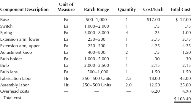
EXHIBIT 5.5 BILL OF MATERIALS WITH BATCH RANGE

An excellent competitive tool for companies that want to adjust their prices to match different production volumes is to maintain a separate database of unit costs for a wide range of production and purchasing volumes. The marketing staff can use this information to conduct what-if analyses for a specific level of sales volume, so that it can estimate, with a fair degree of precision, the profits to be expected at each volume level. Unfortunately, such a database is usually custom-designed, and requires a great deal of research to assemble the data for all relevant volume ranges. Some Japanese companies have taken over a decade to create such systems.

VARIATIONS IN COST BASED ON OVERHEAD

The line item in a BOM that continually raises the most questions from the recipients of cost reports is for overhead cost. They ask if this cost is relevant, what makes up the number, and how it is allocated.

The relevance of overhead costs is entirely dependent on the use to which the cost information will be put. If the report recipient is concerned only with pricing a product to a level near its variable cost, then there is certainly no need for the overhead cost, which can be ignored. However, if the issue is what price to set over the long term in order to cover all fixed costs, then the overhead figure must be included in the calculation.

If the latter reasoning is used, then the controller must delve deeper into the manner in which overhead costs are calculated and allocated, to ensure that only relevant overhead costs are charged on the BOM. There are two factors that go into the production of the overhead number. One is the compilation of the overhead pool, which yields the grand total of all overhead costs that subsequently will be allocated to each product. The second factor is the allocation method that is used to determine how much of the fixed cost is allocated to each unit.

The overhead cost pool can contain a wide array of costs that are related to the production of a specific product in varying degrees. For example, there may be machine-specific costs, such as setup, depreciation, maintenance, and repairs, that have some reasonably traceable connection to a specific product at the batch level. Other overhead costs, such as building maintenance or insurance, are related more closely to the building in which the production operation is housed, and have a much looser connection to a specific product. The overhead cost pool may also contain costs for the management or production scheduling of an entire production line, as well as the costs of distributing product to customers. Given the wide-ranging nature of these costs, it is evident that a hodgepodge of costs are being accumulated into a single cost pool, which almost certainly will result in very inaccurate allocations to individual products.

The allocation method is the other factor that impacts the cost of overhead. Far and away the most common method of allocation is based on the amount of direct labor dollars used to create a product. This method can cause considerable cost misallocations, because the amount of labor in a product may be so much smaller than the quantity of overhead cost to be allocated that anywhere from $1 to $4 may be allocated to a product for every $1 of direct labor cost in it. Given the high ratio of overhead to direct labor, it is very easy for the amount of overhead charged to a product to swing drastically in response to a relatively minor shift in direct labor costs. A classic example of this problem is what happens when a company decides to automate a product line. When it does so, it incurs extra costs associated with new machinery, which adds to the overhead cost pool. Meanwhile, the amount of direct labor in the product plummets, due to the increased level of automation. Consequently, the increased amount of overhead—which is directly associated with the newly automated production line—is allocated to other products whose production has not yet been automated. This means that a product that is created by an automated production line does not have enough overhead cost allocated to it, while the overhead costs assigned to more labor-intensive products is too high.

There are solutions to the problems of excessively congregated cost pools, as well as allocations based on direct labor. One is to split the single overhead allocation pool into a small number of overhead cost pools. Each of these pools should contain costs that are closely related to each other. For example, there may be an assembly overhead cost pool (as noted in Exhibit 5.6) that contains only those overhead costs associated with the assembly operation, such as janitorial costs, the depreciation and maintenance on assembly equipment, and the supervision costs of that area. Similarly, there can be another cost pool (as also noted in Exhibit 5.6) that summarizes all fabrication costs. This pool may contain all costs associated with the manufacture and procurement of all component parts, which includes the costs of machinery setup, depreciation, and maintenance, as well as purchasing salaries. Finally, there can be an overall plant overhead cost pool that includes the costs of building maintenance, supervision, taxes, and insurance. It may not be useful to exceed this relatively limited number of cost pools, for the complexity of cost tracking can become excessive. The result of this process is a much better summarization of costs.

Each of the newly created cost pools then can be assigned a separate cost allocation method that has a direct relationship between the cost pool and the product being created. For example, the principal activity in the assembly operation is direct labor, so this time-honored allocation method can be retained when allocating the costs of the assembly overhead cost pool to products. However, the principle activity in the fabrication area is machine hours, so this becomes the basis of allocation for fabrication overhead costs. Finally, all building-related costs are best apportioned through the total square footage of all machinery, inventory, and related operations used by each product, so square footage becomes the basis of allocation for this cost pool.

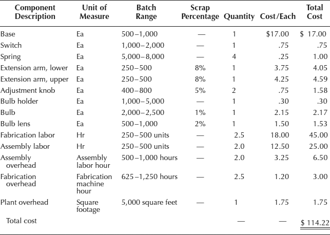
EXHIBIT 5.6 BILL OF MATERIALS WITH MULTIPLE OVERHEAD COSTS

The result of these changes, as noted in Exhibit 5.6, is an altered BOM that replaces a single overhead cost line item with three different overhead costs, each one being allocated based on the most logical allocation measure.

A final issue related to overhead is the frequency with which the overhead cost per unit is calculated. When the controller adds the overhead cost to a BOM, the typical process is to calculate the overhead cost pool, apply an allocation formula, and enter the cost—and not update the resulting figure again for a long time. The updating process can be as laborious as manually accessing each BOM to make an update, or else entering a dollar cost for each unit of allocation (such as per dollar of direct labor, hour of machine time, etc.) into a central computer screen, which the computer system then uses to automatically update all BOMs. In either case, the overhead cost in each BOM will not be updated unless specific action is taken by the controller to update the overhead figures. Consequently, the overhead cost in a BOM must be regularly updated to ensure its accuracy.

By using this more refined set of overhead allocation methods, the accuracy of cost reports can be increased. In particular, it tells managers which cost pools are responsible for the bulk of overhead costs being assigned to specific products. This is information they can use to target reductions in these cost pools, thereby reducing overhead charges.

VARIATIONS IN COST BASED ON TIME

The old adage points out that in the long run, nothing is certain except for death and taxes. This is not precisely true. Also, virtually all costs are variable in the long run. Accountants are good at classifying costs as fixed or variable, but they must remember that any cost can be eliminated if enough time goes by in which to effect a change. For example, a production facility can be eliminated, as can the taxes being paid on it, as well as all of the machinery in it and the people employed there. Though these items may all seem immovable and utterly fixed in the short run, a determined manager with a long-term view of changing an organization can eliminate or alter them all.

Some fixed costs can be converted into variable costs more easily than others. There are three main categories into which fixed costs can fall:

1. Programmable costs. These are costs that are generally considered to be fixed but that can be eliminated relatively easily and without the passage of much time, while also not having an immediate impact on a company's daily operations. An example of such a cost is machine maintenance. If a manager needs to hold down costs for a short period, such as a few weeks, eliminating machine maintenance should not have much of an impact on operations (unless the equipment is subject to continual breakdown!).
2. Discretionary costs. These are costs that are not considered to vary with production volume and that frequently are itemized as administrative overhead costs. Again, these are costs that can be eliminated in the short run without causing a significant impact on operational efficiencies. Examples of discretionary costs are advertising costs and training expenses.
3. Committed costs. These are costs to which a company is committed over a relatively long period, such as major capital projects. Due to the amount of funding involved, the amount of sunk costs, and the impact on production capabilities, these are costs that can be quite difficult to eliminate.

A manager who is looking into a short-term reduction in costs will focus his or her attention most profitably on the reduction of programmable and discretionary costs, since they are relatively easy to cut. If the intention is a long-term reduction, and especially if the size of reduction contemplated is large, then the best type of fixed cost to target is committed costs.

If the manager requesting costing information is undertaking a long-term cost-reduction effort, the controller should go to great lengths to identify the exact nature of all fixed costs in the costing analysis, so that the recipient can determine whether these costs can be converted to variable costs over the long term, or even completely eliminate them.

COST ESTIMATION METHODS

We have covered a number of issues that impact cost. After reviewing the preceding list, one might wonder how anyone ever estimates a cost with any degree of accuracy, given the number of issues that can impact it. In this section, we cover a number of methods, with varying degrees of accuracy and difficulty of use, that can be used to derive costs at different levels of unit volume. These methods are of most use in situations where the costs listed in a BOM are not reliable, due to the impact of outside variables (as noted in the preceding sections) that have caused costs to vary to an excessive degree.

The first and most popular method by far is to have very experienced employees make a judgment call regarding whether or not a cost is fixed or variable, and how much it will change under certain circumstances. For example, a plant manager may decide that the cost of utilities is half fixed and half based on the number of hours that machines are operated in the facility, with this number becoming totally fixed when the facility is not running at all. This approach is heavily used because it is easy to make a determination, and because in many situations the result is reasonably accurate—after all, there is something to be said for lengthy experience! However, costs may be much more or less variable than an expert estimates, resulting in inaccurate costs. Also, experts tend to assign costs to either the fixed or variable categories, without considering that they really might be mixed costs (as in the last example) that have both fixed and variable portions. The problem can be resolved to some degree by pooling the estimates of a number of experts, or by combining this method with the results obtained from one of the more quantitative approaches to be covered shortly in this section.

A more scientific approach is the engineering method. This involves having a qualified industrial engineer team with a controller to conduct exact measurements of how costs relate to specific measurements. For example, this approach may use time-and-motion studies to determine the exact amount of direct labor that is required to produce one unit of finished goods. The result is precise information about the relationship between a cost and a specific activity measure. However, this approach is extremely time consuming, and so is difficult to conduct when there are many costs and activities to compare. Also, the cost levels examined will be accurate only for the specific volume range being used at the time of the engineering study. If the study were to be conducted at a different volume of production, the original costing information per unit produced may no longer be accurate. However, since many businesses operate only within relatively narrow bands of production capacity, this latter issue may not be a problem. A final issue with the engineering method is that it cannot be used to determine the per-unit cost of many costs for which there is no direct relationship to a given activity. For example, there is only a tenuous linkage in the short run between the amount of money spent on advertising and the number of units sold, so the engineering method will be of little use in uncovering per-unit advertising costs. Despite these problems, the engineering method can be a reasonable alternative if confined to those costs that bear a clear relationship to specific activities, and for which there are not significant changes in the level of activity from period to period.

An alternative approach that avoids an intensive engineering review is the scattergraph method. Under this approach, the cost accounting staff compiles activity data for a given period, and then plots it on a chart in relation to the costs that were incurred in the same period. An example of a scattergraph is shown in Exhibit 5.7. In the exhibit, we plot the relationship between the number of units produced and the total variable material cost for the period. The total material cost is noted on the Y axis and the number of units on the X axis. Though there is some variability in the positioning of costs per unit at different volume levels, it is clear that there is a significant relationship between the number of units produced and the total variable material cost. After completing the scattergraph, the controller then manually fits a line to the data (as also noted in the exhibit). Then, by measuring the slope of the line and the point where the line intercepts the Y axis, one can determine not only the variable cost per unit of production, but also the amount of fixed costs that will be incurred, irrespective of the level of production. This is a good quantitative way to assemble relevant data into a coherent structure from which costing information can be derived, but suffers from the possible inaccuracy of the user's interpretation of where the average slope and placement of the line should be within the graph. If the user creates an incorrect Y intercept or slope angle, then the resulting information pertaining to fixed and variable costs will be inaccurate. However, this approach gives the user an immediate visual overview of any data items that are clearly far outside the normal cluster of data, which allows her to investigate and correct these outlying data points, or to at least exclude them from any further calculations on the grounds that they are extraneous. Further, the scattergraph method may result in a shapeless blob of data elements that clearly contain no linearities, which tells the controller that there is no relationship between the costs and activity measures being reviewed, which means that some other relationship must be found. There are two ways to create a more precise determination of the linearity of this information—the high/low method and the regression calculation.

Since the manual plotting of a “best-fit” line through a scattergraph can be quite inaccurate, a better approach is to use a mathematical formula that derives the best-fit line without the risk of operator error. One such method is the high/low method. To conduct this calculation, take only the highest and lowest values from the data used in the scattergram and determine the difference between them. If we use the same data noted in the scatter-graph in Exhibit 5.7, the calculation of the differential would be:

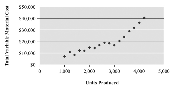
EXHIBIT 5.7 A SCATTERGRAPH CHART

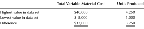
The calculation of the cost per unit produced is $32,000 divided by 3,250, which is the net change in cost divided by the net change in activity. The result is $9.85 in material costs per unit produced.

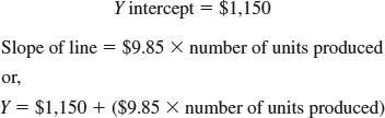
There may also be a fixed cost component to the trend line, indicating the existence of costs that will be present even if no activities occur. This is not the case in the example, since we are focusing on variable material costs. However, it may very well be the case in many other situations. For example, if the preceding trend line were the result of an analysis of machine costs to units produced, we would intuitively know that some machine costs will still occur even if there are no units produced. These costs can include the depreciation on equipment, preventive maintenance, and personal property taxes. We can still use the high/low method to determine the amount of these fixed costs. To do so, we will continue to use the $9.85 per unit in variable costs that we derived in the last example, but we will increase the cost for the lowest data value observed to $11,000. We then multiply the variable cost per unit of $9.85 times the total number of units produced at the lowest observed level, which is 1,000 units, which gives us a total variable cost of $9,850. However, the total cost at the lowest observed activity level is $11,000, which exceeds the calculated variable cost of $9,850 by $1,150. This excess amount of cost represents the fixed costs that will be incurred, irrespective of the level of activity. This information can be summarized into a formula that describes the line:

The obvious problem with the high/low method is that it uses only two values out of the entire available set of data, which may result in a less accurate best-fit line than would be the case if all scattergram data were to be included in the calculation. The problem is particularly acute if one of the high or low values is a stray figure that is caused by incorrect data, and is therefore so far outside of the normal range of data that the resulting high/low calculation will be significantly skewed. This problem can be avoided to some extent if the high and low values are averaged over a cluster of values at the high and low ends of the data range, or if the data are visually examined prior to making the calculation, and clearly inaccurate data are either thrown out or corrected.

A formulation that avoids the high/low calculation's problem of using too few data items is called linear regression. It uses every data item in a data set to calculate the variable and fixed cost components of an activity within a specific activity range. This calculation is best derived on an electronic spreadsheet, which can quickly determine the best-fit line on the scattergram that comes the closest to all data points. It does so by calculating the line for which the sum of all squared deviations between the line and all data elements results in the smallest possible figure. The result is shown in Exhibit 5.8, where a line has been plotted through the scattergram by the computer. A variation on the process is shown in the same graph, which includes a curvilinear regression line that matches the data more closely. The curvilinear approach does not force the computer program to determine a straight line from the available data, thereby revealing trends in the data that may not otherwise be immediately apparent, such as higher or lower variable costs per unit at different volume levels.

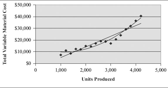
EXHIBIT 5.8 LINEAR AND CURVILINEAR REGRESSION ANALYSIS

The regression calculation method is the most accurate of all the cost prediction models, but suffers from several issues that one must be aware of when creating regression calculations. They are:

• Verify a valid cause-and-effect relationship. Even though the regression analysis may appear to have found a solid relationship between an activity and a cost, be sure to give the relationship a reality test to ensure that it is valid. For example, there is a long-running and completely irrelevant relationship between the length of women's skirts and variations in the stock market. Even though there may be a statistically valid relationship, there is no reason in fact for the relationship to exist, and so there is no reason for changes in the activity to accurately predict stock market volatility in the future. Similarly, make sure that the activity measure being included in a regression analysis bears some reasonable relationship to the cost being reviewed.
• Pick a cost driver with a statistically strong relationship to the activity being measured. No matter how obviously a cost driver appears to relate to an activity from the standpoint of common sense, it may not be suitable if the measured data do not support the relationship. Evidence of a tight relationship is one where the trend line in the regression analysis has a steep slope, and about which the data points are tightly clustered. If this is not the case, another cost driver should be found that results in a better statistical relationship.
• Verify the accuracy of data collection methods. A regression analysis may result in a weak correlation between a cost driver and an activity—not because there is in fact a weak correlation, but because the data collection system that compiles the activity data is not functioning properly. To correct this problem, one should examine the procedures, forms, training, and data entry methods used to accumulate all activity data, and have the system periodically audited to ensure that the correct information is being reported.
• Include all relevant costs. When comparing an activity to a cost, a common problem is to not include costs because they are recorded either in the wrong account or in the wrong time period. In the first case, this requires better attention to how costs are compiled and stored in the accounting system. In the latter case, the easiest way to ensure that costs are included in the correct time period is to lengthen the time period used for the study—for example, from a month to a quarter. By doing so, inter-period changes in costs are eliminated, and the sample size is so much larger that any remaining problems with the timing of costs are rendered statistically insignificant.
• Ensure that the time required is worth the effort. A regression analysis involves the determination of a cost driver, data collection, plotting on a scattergraph to find and correct outlying data items, and then (finally) the actual regression calculation. If the benefit of obtaining this information is less than the not-inconsiderable cost of the effort required to obtain it, then switch to a less accurate and less expensive prediction method that will yield a more favorable cost/benefit ratio.

No matter which of the preceding methods are used, there still will be the potential for errors in costing predictions, given the various problems inherent with each method. To counteract some of these problems, it is useful to combine methods. For example, the linear regression method can derive an accurate formulation of fixed costs and variable costs per unit, but only if the data being used are accurate; by preceding the regression analysis with a review of the data by an expert who can throw out or adjust inaccurate data, the resulting regression analysis will be significantly improved. This same principle can be applied to any of the quantitative measures noted here: Have the underlying data reviewed by experienced personnel prior to running the calculations, and the results will be improved.

NORMAL ACTIVITY

A significant consideration in the control of manufacturing overhead expense through the analysis of variances is the level of activity selected in setting the standard costs. While it has no direct bearing on the planning and control of the manufacturing expenses of each individual department, it does have an impact on the statement of income and expenses (both planned and actual) as well as on the statement of financial position. As to the income statement, it is desirable to identify the amount of manufacturing expense “absorbed” by or allocated to the manufactured product, with the excess expense identified as variance from the standard cost. This variance or excess cost ordinarily should be classified as to cause. As to the statement of financial position, the normal activity level has a direct impact on inventory valuation and, consequently, on the cost-of-goods-sold element of the income statement, in that it helps determine the standard product cost. It should be obvious that the fixed element of unit product costs is greatly influenced by the total quantity of production assumed. Of equal importance is the necessity of a clear understanding by management of the significance of the level selected, because in large part it determines the “volume” variance.

Generally speaking, there are three levels on which fixed standard manufacturing overhead may be set:

1. The expected sales volume for the year, or other period, when the standards are to be applied
2. Practical plant capacity, representing the volume at which a plant could produce if there were no lack of orders
3. The normal or average sales volume, here defined as normal capacity

Some general comments may be made about each of these three levels. If expected sales volume is used, all costs are adjusted from year to year. Consequently, certain cost comparisons are difficult to make. Furthermore, the resulting statements fail to give management what may be considered the most useful information about volume costs. Standard costs would be higher in low-volume years, when lower prices might be needed to get more business, and lower in high-volume years, when the increased demand presumably would tend toward higher prices. Another weakness is that the estimate of sales used as a basis would not be too accurate in many cases.

Practical plant capacity as a basis tends to give the lowest cost. This can be misleading because sales volume will not average this level. Generally, there will always be large unfavorable variances, the unabsorbed expense.

Normal sales volume or activity has been defined as the utilization of the plant that is necessary to meet the average sales demand over the period of a business cycle or at least long enough to level out cyclical and seasonal influences. This base permits a certain stabilization of costs and the recognition of long-term trends in sales. Each basis has its advantages and disadvantages, but normal capacity would seem to be the most desirable under ordinary circumstances.

Where one product is manufactured, normal capacity can be stated in the quantity of this unit. In those cases where many products are made, it is usually necessary to select a common unit for the denominator. Productive hours are a practical measure. If the normal productive hours for all departments or cost centers are known, the sum of these will represent the total for the plant. The total fixed costs divided by the productive hours at normal capacity results in the standard fixed cost per productive hour.

Volume variances can also cause costing problems in an ABC environment. Activity costs are derived by dividing estimated volumes of activity drivers into activity cost pools to derive costs for individual activities. If the estimated volume of an activity driver deviates excessively from the actual amount, then the activity cost applied to a product may significantly alter the product's ABC cost. For example, there are estimated to be 1,000 material moves associated with a product in a month, and the total cost of those moves in a month is $10,000, which is $10 per move. If the actual number of moves associated with the product is 2,000, then the cost per move that is applied to product costs is off by $5 per move. However, if the ABC system collects activity driver volume information for every accounting period, then the volume variance will not occur.

ALLOCATION OF INDIRECT PRODUCTION COSTS

This section discusses the methods for storing and allocating costs in a typical cost accounting system, as well as the types of costs that are typically found in an indirect production cost pool. The discussion is designed to leave the reader with a good understanding of how to organize costs into an adequate cost allocation system.

It is common for a company to have a large amount of overhead costs that are not readily identifiable to a specific product or service. These costs can include engineering, fixed asset charges, general supervision, and quality-related costs. Though it is possible to simply lump these costs into a massive overhead account,” it is irresponsible to do so, because this means that there is minimal identification of or control over what may very well be the largest expense in the company. To attain greater control over these costs, it is best to first group costs into cost pools, from which they can be allocated to various activities.

Most companies still use just one cost pool to allocate costs to activities. This single overhead cost pool is frequently allocated to products based on the labor that goes into making them. For example, if all overhead costs during the period equal $1 million and the total direct labor incurred during that period equals $100,000, then a controller is theoretically justified in charging $10 to a product for every dollar of direct labor cost that it has absorbed. The problems with this allocation approach are that the costs contained in the single cost pool may not directly relate to the product, while the direct labor rate may not be the best way to allocate costs to the product. A better approach is to group costs into different cost pools related to specific activities, and then allocate those costs based better allocation measures. Examples of cost pools are:

• Employee-related costs. These costs can include benefits, the cost of payroll systems, and the entire cost of the human resources and payroll departments. This cost pool should be allocated out to activities based on their use of employees—for example, an activity like production, that normally uses a large proportion of a company's employees, should be charged with a large proportion of this cost pool.
• Equipment-related costs. Many costs directly relate to specific machines or groups of machines, such as depreciation, maintenance, and repairs. These costs can easily be charged back to the machines based on the amount of machine usage. It is common for each machine to have its own cost pool, which can then be charged out to production jobs based on the machine hours used by each job.
• Materials-related costs. There are significant costs associated with storing and moving materials, such as taxes insurance, a warehouse staff, and materials handling equipment. These costs can be charged to specific products based on the square footage occupied by finished goods, as well as by the space taken up by component parts.
• Occupancy-related costs. A building requires expenditures for utilities, repairs, insurance, and a maintenance staff, all of which can be stored in a cost pool and charged out to various activities based on the square footage they require.
• Transaction-related costs. Some activities require a considerable usage of transaction processing expenses, such as order entry time, the time to issue an invoice and collect on it, and procure materials for an order. There are significant staff expenses attached to these activities, which can be charged out based on order size or frequency, or even the number of invoices issued.

All of these cost pools have a different allocation method, because company activities use the costs in different ways. For example, a production job should be charged for the machine hours it uses on a specific machine, rather than direct labor hours, because the machine usage more correctly reflects the job's use of a company asset. Though this may seem like a relatively simple and accurate approach to allocating costs, there are a variety of problems to be aware of:

• New cost-tracking systems needed. A traditional cost allocation system uses only one cost pool, so this revised approach, with multiple pools, requires a different cost roll-up methodology in the general ledger, as well as the storage of information about the different allocation methods to be used. For example, the existing system may not track the usage of a specific machine by all production jobs, which is needed to properly allocate costs from the cost pool.
• Multilevel allocations are probable. Not all cost pools can be charged straight to an activity or customer, because there is no direct relationship. Instead, one cost pool may have to be charged to another cost pool, which in turn is charged to the final activity. For example, the cost pool for occupancy-related costs must first be charged (at least in part) to the machine cost pool, since each machine uses up some building space (which is the usual allocation method for occupancy costs); the enlarged machine cost pool is then charged to an activity.
• Some costs do not fit into any cost pools. There will always be some costs, such as the receptionist's salary or subscriptions, that do not easily fall into the usual cost pools, and which could not justifiably be charged to an activity in any event. These costs should be segregated and tracked; if the total of these costs becomes excessive, there should be a review to determine which costs actually can be shifted to a cost pool—an excessive amount of unallocatable costs leads one to conclude that there are too many costs that are probably not justified in order to run a company.

This section described the most common cost pools used to allocate indirect costs, as well as the allocation methods used to charge the pooled costs out to activities. Though presented in a simplified manner, this should be sufficient information for a controller to construct a simple indirect cost allocation system.

BUDGETARY PLANNING AND CONTROL OF MANUFACTURING EXPENSES

Having discussed those special factors that are important in the proper planning and control of manufacturing expense, we will now review some of the budgetary methods. It should be understood that manufacturing expenses can be controlled through the use of unit standards applied to the expense type or department under consideration. Probably budgetary control is the technique more useful in the overall planning of expense levels, as well as the control phase.

Three types of budgets might be applied in the manufacturing expense area:

1. A fixed- or administrative-type budget
2. A flexible budget, wherein certain expenses should vary with volume handled
3. A step-type budget

Fixed-Type Budget

The fixed-type budget is, as the name implies, more or less constant in the amount of budgeted or allowed expenses for each month. The permitted expense level does change somewhat to reflect a differing volume of manufacturing. Basically, the planning procedure is one wherein the department manager estimates the level of expenses, by account, for each month of the planning period, with some recognition given to expected differing amounts of production. These monthly estimates are subject to review by a superior (with the advice in some instances of the controller or budget director). The control phase consists in comparing actual expense incurred with the predetermined estimate.

An example of a summary planning budget of the fixed type for the manufacturing department is illustrated in Exhibit 5.9. While the budget estimate in this exhibit reflects only the annual and quarterly amounts, in practice the estimate is prepared on a monthly basis.

This fixed type of budget has the advantage of simplicity, and some recognition is given to the small changes in production level. Where production volume is nearly constant, perhaps the method is satisfactory. If the monthly budget in the example is predicated on a volume of 43,333 machine hours (⅓ of 130,000) and the actual level turns out to be 51,000, can the resulting budget comparison be deemed a good control tool? For expenses that are truly fixed, it would be satisfactory. For expenses that should vary by production volume, the “allowed” budget may be inadequate—if such a wide variance happens frequently.

EXHIBIT 5.9 MANUFACTURING EXPENSE—FIXED-TYPE BUDGET

Flexible Budget

The flexible or variable budget recognizes that some expense levels should change as the volume of production varies, and it is the type suggested for proper planning and control of manufacturing expenses in many instances. An illustrative annual planning budget is shown in Exhibit 5.10. An example of a related budgetary control report is presented in Exhibit 5.11.

Basically, the budgetary procedure is:

• By an examination and analysis of the expenses in each department, for each type of expense the budget structure of a fixed amount and a variable rate per factor of variability is determined. For an illustrative structure, see Exhibit 5.10.
• The department manager, when the planned production level is known, applies the budget structure to the planned volume level, probably by month, and arrives at the annual budget. (See Exhibit 5.10).
• The planned budget is reviewed by the manager's supervisors, etc.; after the iterative process is complete, the approved budget becomes part of the manufacturing division budget.
• This budget is incorporated in the company/division annual plan.
• Each month the actual expenses are compared to the flexible budget as applied to the actual volume level experienced. (See Exhibit 5.11).
• Corrective action, if necessary, is taken by the department manager.

For most applications this flexible-type budget probably is the more suitable.

Step-Type Budget

Some companies desire budgets that more or less reflect what expenses should be at particular levels, but wish to avoid a monthly calculation of the allowable budget based on the fixed amount and variable unit rate as in the flexible budget. Rather, the management prefers to establish a budget for each level of activity within a range of possible activity levels. Such a budget is illustrated in Exhibit 5.12.

Budgetary control consists of comparing actual expenses, by account, with the budget level closest to the activity level experienced. Some applications provide for interpolating between budget levels for the allowed budget.

Summarized Manufacturing Expense Planning Budget

In the context of planning, the annual planning budget should be prepared for each department in the manufacturing department, on a responsibility basis. Whatever type of budget is to be used—whether fixed or variable—the department budgets for the expected production level for the plan year should be summarized as part of the annual planning process. A summarized manufacturing expense budget, after completion of the iterative process and approval by the chief production executive, could be in the format reflected in Exhibit 5.13. This planning budget is then used in the process of determining the total cost of goods manufactured. While the illustrated budget is presented on an annual basis only, in fact the budget is prepared to show monthly data.

From a control viewpoint, each month the actual departmental expenses, by type of expense, under the control of the department manager, are compared with the monthly budget, reasons for variance are established, and corrective action taken. A representative departmental control report is shown in Exhibit 5.11, as already commented upon.

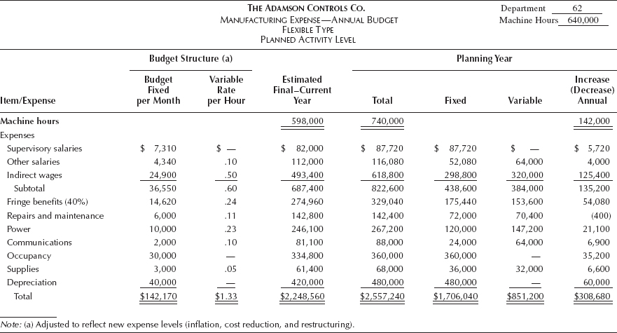
EXHIBIT 5.10 MANUFACTURING EXPENSE—FLEXIBLE BUDGET

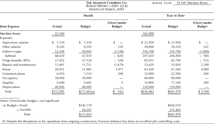
EXHIBIT 5.11 DEPARTMENTAL BUDGET REPORT

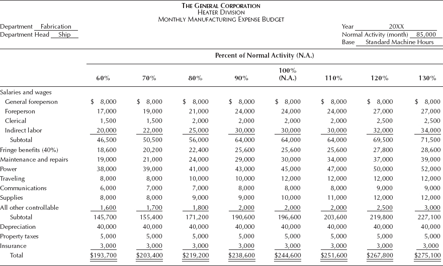
EXHIBIT 5.12 MANUFACTURING EXPENSE BUDGET: STEP TYPE

EXHIBIT 5.13 SUMMARIZED MANUFACTURING EXPENSE BUDGET, BY DEPARTMENT

REVISION OF MANUFACTURING EXPENSE BUDGETS

It is intended that any budget procedure be a useful function. Since the budget structure is founded on certain assumptions, standards, and criteria, these need to be periodically checked. Normally, the expense structure does not change very often, but there will be occasions when the data should be updated, such as when:

• There are major changes in the manufacturing process (e.g., introduction of JIT techniques) such as cellular manufacturing or departmental functions.
• Major changes take place in the salary, wage, or employee fringe benefits package.
• Major organizational changes take place (new departmental structure).
• Major inflationary or other external price changes occur in commodities or services purchased and so forth.

Many of these adjustments can be made in connection with the annual planning cycle. During the interim period, small cost level advances probably can be ignored, but major increases need to be instituted on a timely basis.

SECURING CONTROL OF OVERHEAD

As previously stated, the basic approach in controlling factory overhead is to set standards of performance and operate within the limits of these standards. Two avenues may be followed to accomplish this objective: one involves the preplanning or preventive approach; the other, the after-the-fact approach of reporting unfavorable trends and performance.

Preplanning can be accomplished on many items of manufacturing overhead expense in somewhat the same fashion as discussed in connection with direct labor. For example, the crews for indirect labor can be planned just as well as the crews for direct labor. The preplanning approach will be found useful where a substantial dollar cost is involved for purchase of supplies or repair materials. It may be found desirable to maintain a record of purchase commitments, by responsibility, for these accounts. Each purchase requisition, for example, might require the approval of the budget department. When the budget limit is reached, then no further purchases would be permitted except with the approval of much higher authority. Again, where stores or stock requisitions are the sources of charges, the department manager may be kept informed periodically of the cumulative monthly cost, and steps may be taken to stop further issues, except in emergencies, as the budget limit is approached. The controller will be able to find ways and means of assisting the department operating executives to keep within budget limits by providing this kind of information.

The other policing function of control is the reporting of unfavorable trends and performance. This involves an analysis of expense variances. Here the problem is somewhat different as compared with direct labor or material because of the factor of different levels of activity. Overhead variances may be grouped into the following classifications:

• Controllable by departmental supervision
  • Rate or spending variance
  • Efficiency variance
• Responsibility of top management
  • Volume variance

It is important to recognize the cause of variances if corrective action is to be taken. For this reason, the variance due to business volume must be isolated from that controllable by the departmental supervisors.

Activity-based costing is rarely used for budgeting, but if the controller wishes to use it, then bills of activity and bills of material should be used as the foundation data for standard costs. Multiplying the planned production quantities by the activity costs found in the bills of activity and direct costs found in the bills of lading will yield the bulk of all anticipated manufacturing costs for the budget period. The appropriate management use of budgeted activity costs is to target reductions in the use of activities by various products, as well as to reduce the cost of those activities. For example, the cost of paying a supplier invoice for a part used by the company's product can be reduced by either automating the activity to reduce its cost, or to reduce the product's use of the activity, such as by reducing the number of suppliers, reducing the number of parts used in the product, or grouping invoices and only paying the supplier on a monthly basis.

Analysis of Expense Variances

The exact method and degree of refinement in analyzing variances will depend on the desires of management and the opinion of the controller about requirements. However, the volume variance, regardless of cause, must be segregated from the controllable variances. Volume variance may be defined, simply, as the difference between budgeted expense for current activity and the standard cost for the same level. It arises because production is above or below normal activity and relates primarily to the fixed costs of the business. The variance can be analyzed in more detail about whether it is due to seasonal causes, the number of calendar days in the month, or other causes.

The controllable variances may be defined as the difference between the budget at the current activity level and actual expenses. They must be set out for each cost center and analyzed in such detail that the supervisor knows exactly what caused the condition. At least two general categories can be recognized. The first is the rate of spending variance. Simply stated, this variance arises because more or less than standard was spent for each machine hour, operating hour, or standard labor hour. This variance must be isolated for each cost element of production expense. An analysis of the variance on indirect labor, for example, may indicate what share of the excess cost is due to: (1) overtime, (2) an excess number of workers, or (3) use of higher-rated workers than standard. The analysis may be detailed to show the excess by craft and by shift. As another example, supplies may be analyzed to show the cause of variance as: (1) too large a quantity of certain items, (2) a different material or quality being used, or (3) higher prices than anticipated.

Another general type of controllable variance is the “production” or “efficiency” variance. This variance represents the difference between actual hours used in production and the standard hours allowed for the same volume. Such a loss involves all elements of overhead. Here, too, the controller should analyze the causes, usually with the assistance of production personnel. The lost production might be due to mechanical failure, poor material, inefficient labor, or lack of material. Such an analysis points out weaknesses and paves the way to corrective action by the line executives.

The accounting staff must be prepared to analyze overhead variances quickly and accurately to keep the manufacturing supervision and management informed. The variance analysis should relate to overhead losses or gains for which unit supervision is responsible and include such features as:

• The expenditure or rate variance for each cost element as an over or under the budget condition for the reporting period and year to date. The budgeted amount for controllable expenses may be calculated by multiplying the operating hours by the standard rate per cost element and compared to actual.
• The departmental variance related to the level of production.
• The amount of fixed costs, even though the particular supervisor may not be responsible for the incurrence.
• Interpretative comments as to areas for corrective action, trends, and reasons for any negative variances.

It is not sufficient just to render a budget report to the manufacturing supervision; this group must be informed about the reasons for variances. The information must be communicated and a continuous follow-up must be undertaken to see that any unfavorable conditions are corrected. This may take the form of reviewing and analyzing weekly or even daily reports. Abnormal conditions such as excess training, overtime, absenteeism, and excessive usage of supplies must be isolated and brought to the attention of the responsible individuals who can take remedial action. There also may be other data available such as repair records, material and supplies usage reports, personnel statistics—including turnover and attendance records that are useful.

Responsibility must be established for all significant variances in a timely manner so that appropriate corrective action is taken.

Incentives to Reduce Costs

It has been stated repeatedly that costs are controlled by individuals. In the control of manufacturing expenses, as in the case of direct labor and material, a most important factor is the first-line supervision. As representatives of management who are on the scene observing production the first-line supervisors can detect immediately deficient conditions and take action or influence the utilization of resources. Reports showing the performance of this group are of great assistance. However, the experience of many companies has shown that standard costs or budgets covering indirect costs are a more effective management tool when related to some type of incentive or financial reward. Usually, this incentive takes the form of a percentage of the savings or is based on achieving a performance realization above some predetermined norm. If a supervisor participates in the savings from being under the budget it is a powerful force in obtaining maximum efficiency. Since variances will fluctuate from month to month, it is advisable to consider an incentive plan for supervision on a cumulative performance basis—a quarter or a year.

INDIRECT LABOR: A MORE PRECISE TECHNIQUE

Indirect labor often is one of the largest controllable elements of manufacturing expense and therefore may warrant a special review. In the examples provided earlier in this chapter, an acceptable cost level for this type of expense was determined by measuring the historical cost against a factor of variability such as standard machine hours or direct labor hours. Sometimes the correlation may not be as close as desired and a more analytical technique may be necessary—which involves the aid of industrial or process engineers. The method, which closely resembles the calculation of the required direct labor for any given manufacturing operation, essentially is:

• The engineers study the specific function to be performed by the departmental indirect labor crew, including the exact labor hours required at differing activity levels.
• An activity base is selected, such as standard machine hours, that would be a fair and easily determinable measure of just what labor hours are needed for each function of the indirect labor crew.
• Estimates are made as to just what portion of the crew is fixed, and what portion can be treated as variable (perhaps by performing other functions), and the related labor hours are determined.
• The hours data are costed (by the cost accountants), the fixed budget allowance determined, and the variable rate calculated per unit of activity.

The process is summarized on the cost worksheet in Exhibit 5.14. First, the technical data are summarized, and then the cost bases are calculated.

Where deemed appropriate, this more exact method can be used in arriving at the flexible budget base.

OTHER ASPECTS OF APPLYING BUDGETARY CONTROL

In applying budgetary control to manufacturing expenses, an alert controller will generate ideas of how to make the budget report more usable to those managers who use it. There are many techniques that can be found; however, in any case it takes good communication. Normally, accountants will develop budgets in terms of dollars or value. Sometimes, production managers cannot relate their operations to monetary units. In most cases they think and manage in terms of labor hours. If this is more understandable, the budget can easily be stated in terms of labor hours per standard labor hours or some other factor. The budgeted allowances of other expenses may be expressed in units of consumption—kilowatt hours of power, gallons of fuel, tons of coal, pounds of grease, and so on.

One of the purposes of budgetary control is to maintain expenses within the limits of income. To this end, common factors of variability are standard labor hours or standard machine hours—bases affected by the quantity of approved production. If manufacturing difficulties are encountered, the budget allowance of all departments on such a base would be reduced. The controller might hear many vehement arguments by the maintenance foreperson, for example, that the budget should not be penalized because production was inefficient or that plans once set cannot be changed constantly because production does not come up to expectations. Such a situation may be resolved in one of at least two ways: (1) the forecast standard hours could be used as the basis for the variable allowance, or (2) the maintenance foreperson could be informed regularly if production, and therefore the standard budget allowance, will be under that anticipated. The first suggestion departs somewhat from the income-producing sources but does permit a budget allowance within the limits of income and does not require constant changes of labor force over a very short period. The second suggestion makes for more coordination between departments although it injects the element of instability to a slight degree.

Extraordinary or unanticipated expenditures of a manufacturing expense nature must frequently be made. These may fall well without the scope of the usual budget, even when the cumulative yearly condition is considered. In such instances, and if the expenditure is considered necessary and advisable, a special budget allowance will be made over and above the usual budget—something superimposed on the regular flexible budget structure.

Another point should not be overlooked by the accounting staff: The important consideration is not how flexibility is introduced into the standard or budget but rather that it is injected. Whether charts or tables are used to determine the allowable budget on a more or less automatic basis or whether the budget is adjusted monthly or quarterly on the basis of special review in relation to business volume is not too essential, because either method can be successfully employed. The major consideration is that of securing an adequate measuring stick that also keeps expenses at the proper level in relation to activity or income.

EXHIBIT 5.14 ENGINEERING-BASED INDIRECT LABOR BUDGET STRUCTURE

OTHER CONTROL PROCEDURES

The budgetary process has been emphasized for control of manufacturing overhead expenses in this chapter for these reasons:

• It more closely recognizes the cost behavior of the specific types of expense through its fixed and variable expense structure determination.
• It not only addresses the control process, but also is a planning device.
• It tends to promote coordination among functions.

There will be occasions when, for whatever reason, the top management and/or functional management does not wish to adopt budgetary procedures. Under these circumstances, in some departments other standards may be employed. In other instances, selected standards may supplement the budget standards. In fact, it is in the manufacturing function that standards were first employed in the control of not only direct labor and direct material, but also many of the indirect expenses.

Such a system involves the establishment of standards (see Chapter 2) and the comparison of actual expenses—either individual accounts, or departmental totals—against such standards, and the taking of corrective action where appropriate. Many manufacturing executives in particular industries know from observation that certain expense relationships are the key to a profitable operation. Their experience has led to the use of a number of standards or standard relationships for manufacturing expenses. These ratios are usually collected and distributed by industry trade associations or magazines devoted to the affairs of specific industries. Some comparisons often used, or trends followed, are shown in Exhibit 5.15.

For any significant expenses, trends can often be observed in the absolute and in relationship to selected or total manufacturing expenses.

ROLE OF THE CONTROLLER

Much has been said about the technique of setting manufacturing expense budgets or standards, but little mention has been made about who prepares the budgets and applies them. This duty is usually delegated to the controller and staff and understandably so. Past experience is an important factor in setting expense budgets. An analysis of expenses and their behavior in relation to volume is required, and the principal source of information is the accounting records. The accountants are the best qualified to make these analyses of the historical information. Then, too, the accounting staff usually possesses the necessary technical qualifications for organizing the data into the desired shape. Furthermore, the approach must be objective, and the independent position of the accounting department makes it suitable for the setting of fair standards or budgets.

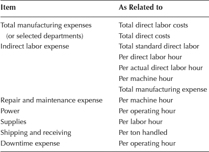
EXHIBIT 5.15 SAMPLE EXPENSE COMPARISONS

Although the controller “carries the ball” in preparing the budgets, he is only part of the team. Successful control of manufacturing expenses requires the cooperation of the operating departments' supervisors who are charged with the responsibility of meeting their budgets. For this reason, among others, each supervisor should agree to the budget before it is put into effect. Moreover, each supervisor's experience and knowledge of operating conditions must be utilized in the preparation of the budget. The controller and staff act as coordinators in seeing that the job gets done reasonably well and that it is accomplished on time.

The role of the controller and staff in the accounting for, and planning and control of, manufacturing expenses may be summarized in this fashion. The controller should:

• Provide that expenses are accumulated in such account categories that control is reasonably simple; that is, the natural expense groupings should originate from the same sources, or a comparable method of control or time or point of control should be employed. Thus, repairs done by outside sources and controlled on a purchase order basis, perhaps should be isolated from in-house repairs that are controlled by requisition.
• Arrange the departmental accounts on a responsibility basis, by natural expense classifications, so that costs are accumulated according to the authority delegated to plan and control the expenses. This categorization also should permit the accumulation of product costs in a suitable manner.
• Where a budgetary process is in effect, arrange that the procedure facilitates the preparation of the planning budget in an effective and timely manner (by provision of adequate instructions, forms, schedules, etc.); and that the control procedure provides a timely accumulation of actual expenses, compared with budget, together with reasons for any significant departure from plan, if known.
• Provide reasonable assistance to department managers in their preparation of the annual plan or budget (including requested analyses), and in searching out causes of standard deviation and perhaps methods of correction.
• Where flexible budgets are in use, either identify, or assist in the identification of, the fixed and variable portions.
• Where budget structures need revision by reason of changed expense levels (inflation, etc.) or new manufacturing processes, see that timely revisions are made to the end that the budgets are useful and not outdated.
• Evaluate the planned level of manufacturing expenses in the process of consolidating and testing the annual plan.
• If budgetary procedures, for whatever reason, are not used, see if some other sort of standard application may be of value in planning and controlling the manufacturing expenses.
• Determine that the costing methods provide reliable and acceptable accumulation and allocation by cost object—product, department (as to service operations), and so forth—and that variances are properly analyzed.

REPORTS FOR MANUFACTURING EXECUTIVES

Scope of Coverage

The supervisory staff of the production organization extends over several levels of authority and responsibility from the assistant foreperson, foreperson, general foreperson, division head, plant superintendent, and so on, up to the works manager. Likewise, the matters the supervisory staff controls relate to materials, labor, and overhead, and each of these subjects has special aspects to be reported on. Production reports must cover a wide field of both reader and subject matter. Effective production control is possible only when the production executives are aware of the necessary facts related to the plant operations, and the higher the executive the more reliance on reports instead of personal contacts and observations. As a result, a system of reports has been developed in most industrial organizations for presenting the pertinent facts on the production activities.

It will bear mentioning that the recent developments in computer hardware and software (programs) permit an improved monitoring of operations. Information on some activities must be, and is, available on a real-time basis. With the advent of personal computers, interesting combination reports consisting of commentary, tabulations, and graphs in an inviting appearance are now possible.

The number of variance reports that are used by manufacturing management will decline as cellular manufacturing becomes the standard form of production. Since cellular manufacturing uses minimal work-in-process (WIP), month-end variance reports from the accounting department will arrive far too late for the information to be useful. For example, if a machine produces a part out of specification, then a cellular layout will immediately detect the problem, because the part will not be hidden in a pile of WIP. Consequently, management can detect and correct the problem immediately without the need for a report.

Types of Reports on Actual Performance

The reports will differ from industry to industry from company to company so that no standardized reports can be set for business generally. However, they may be divided into two general categories according to their purpose. These may be classified as (1) control reports and (2) summary reports. As the name implies, control reports are issued primarily to highlight substandard performance so that corrective action may be taken promptly. These reports deal with performance at the occurrence level and are therefore usually detailed in nature and frequent in issuance. On the other hand, summary reports show the results of performance over a longer period of time, such as a month, and are an overall recapitulation of performance. They serve to keep the general executives aware of factory performance and are, in effect, a summary of the control reports.

Indicative of the subjects the reports to production executives may cover, including direct and indirect costs for which the executive may be responsible, are:

• Material
  • Inventories
  • Spoilage and waste
  • Unit standard costs
  • Material consumed
  • Actual versus standard usage
• Labor
  • Total payroll
  • Unit output per labor hour
  • Total production in units
  • Average hourly labor rates
  • Overtime hours and costs
  • Bonus costs
  • Turnover
  • Relationship of supervisory personnel to direct labor
  • Actual and standard unit and total labor costs
• Overhead
  • Actual versus budgeted costs
  • Idle facilities
  • Maintenance costs
  • Supplies used
  • Cost of union business
  • Subcontracted repairs
  • Ratio of indirect to direct labor

In a production environment that has adopted just-in-time (JIT) manufacturing systems, reports will no longer include standards, because JIT assumes that most cost improvements can be managed in the design phase, not in the production phase, and that collecting variance information costs more in effort than is gained in tangible results. A set of JIT reports would include:

• Inventory turnover
• Unit output per labor hour
• Total production in units
• Staff turnover
• Actual purchased costs versus planned costs
• Inventory accuracy
• Bill of material accuracy
• Bill of activities accuracy

Presentation of Data

Most production executives will make good use of data bearing on their operations provided three fundamental rules are followed:

1. The reports should be expressed in the language of the executive who is to use them and in the form preferred by him.
2. Reports should be submitted promptly enough to serve the purpose intended. Control reports are of little value if issued too late to take corrective action.
3. The form and content of the report should be in keeping with the responsibility of the executive receiving it. Minor executives are interested in details, whereas higher executives are interested in departmental summaries, trends, and relationships.

Some of the reports prepared by the accounting department will be on costs, and others will be expressed in nonfinancial terms. Some may be narrative; others will be in tabular or graphic form. But all should follow the principles just set forth.

EXHIBIT 5.16 LABOR ANALYSIS REPORT

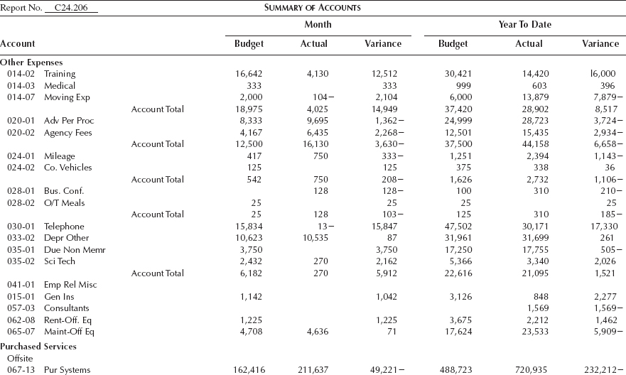
EXHIBIT 5.17 FACTORY OVERHEAD BUDGET REPORT

Illustrative Reports

As indicated previously, indirect manufacturing costs have increased significantly, resulting in the need for better visibility and control of these expenses. Exhibits 5.16 through 5.18 are examples of reports that may be adapted to a particular company or type of manufacturing operation.

Exhibit 5.19 provides an analysis of weekly and year-to-date hours and costs of the indirect labor and related fringe costs of a manufacturing department.

EXHIBIT 5.18 COMPARATIVE COST HISTORY CHART

EXHIBIT 5.19 TREND ANALYSIS CHART

Exhibit 5.20 is a summary and analysis of the monthly and year-to-date expenses for the activity of three manufacturing expense accounts being monitored: supplies, purchased services, and “other” expenses.

EXHIBIT 5.20 TREND ANALYSIS CHART