The Six Classic Orbital Elements

The six classic elements include terms that describe the shape of an orbit (semi-major axis a and eccentricity e), terms that define its position relative to the Earth’s equator and poles (inclination i and argument of perigee w), a term that ties the orbit to our calendar (longitude of the ascending node O), and a final item that says, for the defined orbit, how far along it is (usually mean anomaly, but also can be true anomaly or angle from last perigee passage or time from last perigee passage or time of periapsis passage).

1. a = semi-major axis = size

2. e = eccentricity = shape

3. i = inclination = tilt

4. ω = argument of perigee = twist

5. Ω = longitude of the ascending node = spin

6. v = mean anomaly = where in orbit

Shown here is “Orbit1” by Lasunncty (talk) (licensed under CC BY-SA 3.0 via Wikimedia Commons):

It is not so important that you understand the full meaning of these elements (you can read more online to learn that), but that you accept that these six elements fully define an orbit and its current position.

You can convert any state vector (r,v) to its equivalent orbital elements, and you can convert any orbital elements to a state vector. The state vector says, “Here is a direct line to the object, now,” and the orbital elements are a tool that lets you predict any future state vector. They work well together.

One neat property of the orbital elements is that an orbit’s period P (time to complete one full 360 lap) is proportional to its semi-major axis a (its size). p² = k a³, where the constant k depends on the units used for a and p (and the mass of the object being orbited around; k is different for orbiting Jupiter versus orbiting the Earth, for example). This means that if you know a, you also know the period of the orbit—and vice versa.

TLEs

Orbital elements are often exchanged in NASA’s TLE format, covered in Book 1, DIY Satellite Platforms. Here is a short definition of the specification, excerpted from AMSAT.org, in part because AMSAT is the definitive source for amateur satellite work, and in part because a specification or definition is best quoted to avoid introducing errors. It is a primarily intended for computers rather than people, in that it has a fixed format and there are no labels in the actual data. From AMSAT.org, here is the format and the key for translating it:

1 AAAAAU YYLLLPPP  BBBBB.BBBBBBBB  .CCCCCCCC  DDDDD-D  EEEEE-E F GGGGZ
2 AAAAA  HHH.HHHH III.IIII JJJJJJJ KKK.KKKK MMM.MMMM NN.NNNNNNNNRRRRRZ

Key

[1] - Line #1 label
[2] - Line #2 label
[AAAAA] - Catalog Number assigned sequentially (5-digit integer from 1 to 99999)
[U] - Security Classification (U = Unclassified)
[YYLLLPPP] - International Designator (YY = 2-digit Launch Year; LLL = 3-digit Sequential Launch of the Year; PPP = up to 3 letter Sequential Piece ID for that launch)
[BBBBB.BBBBBBBB] - Epoch Time--2-digit year, followed by 3-digit sequential day of the year, followed by the time represented as the fractional portion of one day
[.CCCCCCCC] - ndot/2 Drag Parameter (rev/day2)--one half the first time derivative of the mean motion. This drag term is used by the SGP orbit propagator.
[DDDDD-D] - n double dot/6 Drag Parameter (rev/day3)--one sixth the second time derivative of the mean motion. The "-D" is the tens exponent (10-D). This drag term is used by the SGP orbit propagator.
[EEEEE-E] - Bstar Drag Parameter (1/Earth Radii)--Pseudo Ballistic Coefficient. The "-E" is the tens exponent (10-E). This drag term is used by the SGP4 orbit propagator.
[F] - Ephemeris Type--1-digit integer (zero value uses SGP or SGP4 as provided in the Project Spacetrack report.
[GGGG] - Element Set Number assigned sequentially (up to a 4-digit integer from 1 to 9999). This number recycles back to "1" on the update following element set number "9999."
[HHH.HHHH] - Orbital Inclination (from 0 to 180 degrees).
[III.IIII] - Right Ascension of the Ascending Node (from 0 to 360 degrees).
[JJJJJJJ] - Orbital Eccentricity--there is an implied leading decimal point (between 0.0 and 1.0).
[KKK.KKKK] - Argument of Perigee (from 0 to 360 degrees).
[MMM.MMMM] - Mean Anomaly (from 0 to 360 degrees).
[NN.NNNNNNNN] - Mean Motion (revolutions per day).
[RRRRR] - Revolution Number (up to a 5-digit integer from 1 to 99999). This number recycles following revolution number 99999.
[Z] - Check Sum (1-digit integer). Both lines have a check sum that is computed from the sum of all integer characters on that line plus a "1" for each negative (-) sign on that line. The check sum is the modulo-10 (or ones digit) of the sum of the digits and negative signs.

As an example, here is a TLE for the X-Ray Timing Explorer (XTE) satellite telescope (now long since deorbited). I include the common (but optional) extra first line designating the mission name (XTE):

XTE
1 23757U 95074A 11333.55435324 .00010246 00000-0 30421-3 0 5229
2 23757 022.9893 121.5427 0007734 071.5825 288.5466 15.321190098829520

Not human-readable, but that is not the point. TLEs are designed so software can easily read the fixed-format information and operate on it. As long as you adhere to the standard, you can get TLEs from any authoritative source and your orbit prediction software will be able to use it. You can get TLEs for just about every tracked satellite from Space-Track, which is chartered by the US Department of Defense to distribute TLEs.

Orbit Determination

So where do TLEs come from? Most people will wait until NORAD/US Space Command releases their orbit data. However, there are five common ways to determine, from observations, the orbital elements. The first method is direct ranging using radar, which is very handy if you own your own radar installation but usually out of the realm of the amateur. The other four are mathematical methods where you make multiple observations of the satellite during one orbit, then use the appropriate mathematics to derive the orbital parameters. These four methods are triangulation, Gauss’s Method, Lambert’s Problem, and the Gibbs Method.

Direct ranging using radar (with Doppler shift), gives you the state vector (r,v) at some known time t. With this, you can derive the orbit because each orbit is unique and independent of the mass of the spacecraft. As mentioned back in Book 1, DIY Satellite Platforms, a satellite’s orbit does not depend on its mass, only its position and velocity. Both the ISS and a CubeSat next to it will orbit identically. This is why, when they eject CubeSats from the ISS, they give the CubeSats a little velocity kick—so they won’t remain right next to the ISS.

Using the radar timing to derive the distance plus the Doppler shift on the radar to get the velocity, you obtain a position and velocity of the satellite relative to the radar station. Add some geometry based on your latitude and longitude, and you obtain the exact state vector (r, v) for the satellite. This is beyond most non-radar-owning amateurs, but is the method our various governments use to track space items. If you don’t have this, you can use a series of ground observations to deduce the orbit. Which method you use depends on that data you can gather.

The remaining methods use multiple ground observations of the satellite during one orbital path. If, from the ground, you can observe the altitude (height above horizon) and azimuth (compass angle), or alternately the astronomical right ascension and declination, of a satellite, you know it is somewhere along that line of sight but you don’t know how far it is.

Triangulation consists of using two simultaneous measurements of an object from two different ground locations to geometrically calculate the object’s exact position. Each observation is one side of a triangle; the line connecting your two observers is the third side. Knowing these three sides and the angles involved, you can use triangle geometry to get the exact position. Therefore, two observers can get a single r vector for a satellite, if they are well coordinated in gathering their data. Satellites zip across the sky quickly, and triangulation requires the measurements be at the exact same time, but this is doable.

If you take three different observations of the object, you can use Gauss’s Method to deduce the complete orbital elements. This is the oldest and roughest method. Code to solve Gauss’s Method exists online and in orbital mechanics textbooks.

If you use radar or communications ranging or triangulation to get the distance, you have a position vector. With two exact position vectors (direction plus the distance to it) and the flight time between them, Lambert’s Problem is an algorithm that will give you the complete orbital elements. With three position vectors but no time information on when the data was taken, you can use the Gibbs Method (implemented in software) to derive the velocity vector v and fully define its state vector. Again, code to solve both is easily found. You now know its orbit.

Satellite Time

Your satellite will probably not know what time it is. It doesn’t have to. You can imagine your satellite is in its own time zone. It is not important what time is on its internal clock, only that you know the offset between your satellite time and terrestrial UT.

When your satellite first powers up, it will have a default start time on its internal clock. This is the equivalent of a newly plugged in alarm clock reading 00:00. You need to record this time and compare it to your ground time. This gives you your clock offset.

While you could reprogram the satellite clock to the current time, this is not recommended. First, it is hard to do this accurately, and second, you have to know exactly when you sent the command plus how long it took the satellite to react to the command and reprogram. It’s also totally unnecessary. Instead, just let the satellite keep its own time, and remember its offset.

For example, if your spacecraft powers up at 17:57UT on Nov 14, 2014, but thinks it started at 12:00 Nov 1, 2014, you now know its offset is that the satellite is running 14 days and 5:57 hours behind your real time. Keep that offset and don’t mess with the satellite clock, because it’s unnecessary to do so and brings absolutely no advantage. Just let the clocks run as they are.

Relativity does alter time. Two objects moving at different speeds or facing a different amount of gravity will find out their clocks run at different rates. The two relativity factors (velocity and gravity) operate in opposite directions, so it turns out the ISS clocks run slower than on Earth (high velocity, roughly the same gravity), while GPS clocks at geosync orbits run faster (slower, further from gravity). The correction can be predicted, but it is easier to just periodically check the clocks against each other and update the offset.

The one implication for commanding your satellite is that if you have any timed commands you wish to do (anything programmed other than do this as soon as you receive this transmission), you need to make your command load match the spacecraft clock/date, not your ground date.

Most larger missions will, in their spacecraft software, include a data item of this offset so the spacecraft is aware of the time shift. For CubeSats, which typically run smaller processors with more immediate “do this as soon as told” commanding, this may not be necessary.

Reboots are another factor to consider. If your satellite reboots itself, either on command or due to radiation damage or a safehold event, the spacecraft clock might (yet again) reset itself to a new time. Just update your offset and you are good to go.

Contact Passes

Your operational flow sequence is to build a schedule for contacts, consisting of:

1. Acquisition of satellite (AOS, also called acquisition of signal)—the time the satellite is above the horizon and expected treeline, and thus visible to your station

2. Location at AOS (relative to your station)

3. Loss of satellite/signal (LOS)—the time the satellite drops below the treeline and/or horizon and is no longer visible

4. Location of LOS

5. Path of satellite

This is easier done in software. Briefly, orbits by definition are a fully predictive path. The most common reference frame for the orbit coordinates is the geocentric frame. Software is used to map this to your local position on the Earth (the topocentric frame), and thus translate the satellite’s position into either an azimuth (compass direction to face) and altitude (height above the horizon), or a right ascension, declination pair (sky coordinates to point at), that your system can then track.

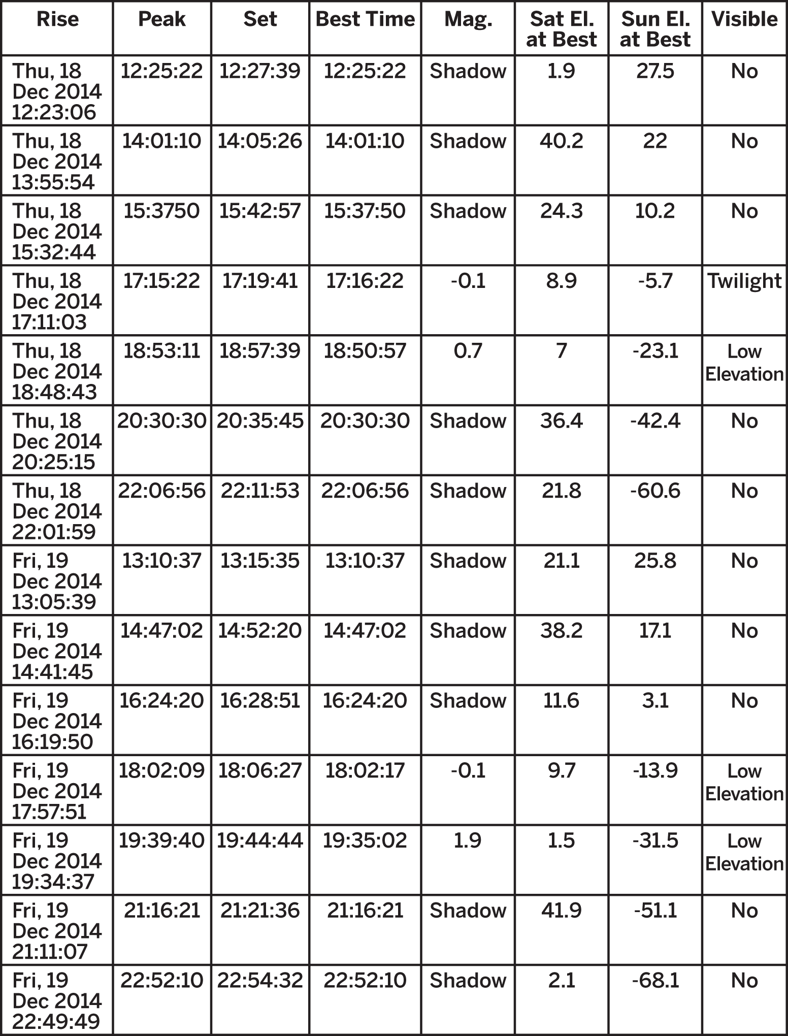
From the predictive elements you can visualize the ground tracks, and also generate a handy table of when your satellite is visible for a specific ground station. Here’s a sample set of data for the ISS for a typical day, generated by SATFLARE. For December 18th and 19th, there are seven consecutive passes per day ranging from two to five minutes. If you rule out passes below five minutes, you get four good passes per day. The following shows a sample set of data for the ISS on a typical day: