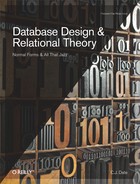
In this chapter, I want to clarify certain general aspects of further normalization before we start getting into specifics (which we’ll do in the next chapter). I’ll begin by taking a closer look at the sample value of relvar S from Figure 1-1 (repeated for convenience in Figure 3-1 below).
Recall now that the functional dependency (FD)
{ CITY } → { STATUS }holds in this relvar (I’ve included an arrow in the figure to suggest this fact). Because that FD holds,[21] it turns out that the relvar is in second normal form (2NF) but not third (3NF). As a consequence, the relvar suffers from redundancy; to be specific, the fact that a given city has a given status appears many times, in general. And the discipline of further normalization—which from this point on I’ll abbreviate most of the time to just normalization, unqualified—would therefore suggest that we decompose the relvar into two relvars SNC and CT of lesser degree, as indicated in Figure 3-2 (which shows, of course, values for those relvars corresponding to the sample value shown for relvar S in Figure 3-1).

Points arising from this example:
First, the decomposition certainly eliminates the redundancy—the fact that a given city has a given status now appears exactly once.
Second, the decomposition process is basically a process of taking projections—the relations shown in Figure 3-2 are each projections of the relation shown in Figure 3-1.[22] In fact, we can write a couple of equations:
     SNC  =  S { SNO , SNAME , CITY }
     CT   =  S { CITY , STATUS }
(Recall from Chapter 2 that the Tutorial D syntax for projection takes the form r{A1,...,An}, where r is some relational expression and A1, ..., An are attribute names.)[23]
Third, the decomposition process is nonloss (also called lossless)—no information is lost in the process, because the relation shown in Figure 3-1 can be reconstructed by taking the join of the relations shown in Figure 3-2:
S = JOIN { SNC , CT }(Tutorial D syntax again.) Thus, we can say the relation in Figure 3-1 and the pair of relations in Figure 3-2 are information equivalent—or, to state the matter more precisely, for any query that can be performed against the relation of Figure 3-1, there’s a corresponding query that can be performed against the relations of Figure 3-2 (and vice versa) that produces the same result. Clearly, such “losslessness” of decompositions is an important property; whatever we do by way of normalization, we certainly mustn’t lose any information when we do it.
It follows from the foregoing that just as projection is the decomposition operator (with respect to normalization as conventionally understood), so join is the corresponding recomposition operator.
So far, so good; this is all very familiar stuff. But now I want to point out that if you’ve been paying careful attention, you might reasonably accuse me of practicing a tiny (?) deception ... To be specific, I’ve considered what it means for a decomposition of relations to be nonloss; but normalization, which is what we’re supposed to be talking about, isn’t a matter of decomposing relations, it’s a matter of decomposing relvars.
Suppose we do decide to perform the suggested decomposition of relvar S into relvars SNC and CT. Observe now that I really am talking about relvars and not relations; for definiteness, however, let’s assume those relvars have the sample values shown in Figure 3-1 and Figure 3-2, respectively. For definiteness again, let’s focus on relvar CT specifically. Well, that relvar is indeed a relvar—I mean, it’s a variable—and so we can update it. For example (using the shorthand notation for tuples introduced in Chapter 2), we might insert the tuple:
( 'Rome' , 10 )
But after that update, relvar CT contains a tuple that had no counterpart in relvar S (it doesn’t have a counterpart in relvar SNC either, come to that). Now, such a possibility is often used—indeed, Codd used it himself in his very first papers on normalization (see Appendix C)—as an argument in favor of doing the normalization in the first place: The normalized, two-relvar design is capable of representing certain information that the original one-relvar design isn’t. (In the case at hand, it can represent status information for cities that currently have no supplier located in them.) But that same fact also means that the two designs aren’t really information equivalent after all, and moreover that relvar CT isn’t exactly a “projection” of relvar S after all[24]—it contains a tuple that isn’t a projection of, or otherwise derived from, any tuple in relvar S.[25] Or rather (and perhaps more to the point), CT isn’t a projection of the join of SNC and CT, either, and so that join “loses information,” in a sense; to be specific, it loses the information that the status for Rome is 10.[26]
A similar situation arises if we delete the tuple
( 'S5' , 'Adams' , 'Athens' )
from relvar SNC. After that update, we could say, a trifle loosely,[27] that relvar S contains a tuple that has no counterpart in relvar SNC (though it does have one in relvar CT). So again the two designs aren’t really information equivalent; and this time relvar S isn’t exactly a “join” of relvars SNC and CT, since it contains a tuple that doesn’t correspond to any tuple in relvar SNC.
The two designs are thus not information equivalent after all. But didn’t I say earlier that “losslessness” of decompositions is an important property? Don’t we generally assume that if Design B is produced by normalizing Design A, then Design B and Design A are supposed to be information equivalent? What exactly is going on here?
In order to answer these questions, it’s helpful to look at the relvar predicates. The predicate for SNC is:
And the predicate for CT is:
City CITY has status STATUS.
Now suppose it’s possible for a city to have a status even if no supplier is located in that city; in other words, suppose it’s possible for relvar CT to contain a tuple such as (Rome,10) that has no counterpart in relvar SNC.[28] Then the design consisting of just relvar S is simply incorrect. That is, if it’s possible for a true instantiation to exist of the predicate City CITY has status STATUS without there existing—at the same time and with the same CITY value—a true instantiation of the predicate Supplier SNO is named SNAME and is located in city CITY, then a design consisting just of relvar S doesn’t faithfully reflect the state of affairs in the real world (because that design is incapable of representing the status for a city in which no supplier is located).
Similarly, suppose it’s possible for a supplier to be located in a city even if that city has no status; in other words, suppose it’s possible for relvar SNC to contain a tuple, say (S6,Lopez,Madrid), that has no counterpart in relvar CT. Then, again, the design consisting just of relvar S is simply incorrect, because it requires every city in which a supplier is located to have some status.
Here’s another way to look at the foregoing argument. Suppose the design consisting just of relvar S did faithfully reflect the state of affairs in the real world after all. Then relvars SNC and CT would be subject to the following integrity constraint (“Every city in SNC appears in CT and vice versa”):
CONSTRAINT ... SNC { CITY } = CT { CITY } ;But this constraint—which is an example of what I’m later going to be calling an equality dependency or EQD—manifestly isn’t satisfied in the example under discussion. Note: For simplicity, I haven’t bothered to give this constraint a name, as you can see. Indeed, I’ll omit such names from all of my examples in this book from this point forward, except where there’s some compelling reason to do otherwise.
To sum up, we see that normalization can be (and is) used to address two rather different problems:
It can be used to fix a logically incorrect design, as in the example discussed earlier in this section. Exercise: Do issues analogous to those raised in that example apply to the STP example from the section THE PLACE OF DESIGN THEORY in Chapter 1? (Answer: Yes, they do.)
It can be used to reduce redundancy in an otherwise logically correct design. (Obviously a design doesn’t have to be logically incorrect in the foregoing sense in order to display redundancy.)
Much confusion arises in practice because these two cases are often not clearly distinguished. Indeed, most of the literature focuses on Case 2—and for definiteness I’ll assume Case 2 myself in what follows, where it makes any difference—but please don’t lose sight of Case 1, which in practice is at least as important, if not more so.
I should point out further that, strictly speaking, the terminology of projections and joins applies only to Case 2. That’s because in Case 1, as we’ve seen, the “new” relvars aren’t necessarily projections of the “old” one, nor is the “old” one necessarily the join of the “new” ones (if you see what I mean). In fact, what does it mean to talk about projections and joins of relvars (as opposed to relations) anyway? Well, as I’ve written elsewhere:[29]
By definition, the operators projection, join, and so on apply to relation values specifically. In particular, of course, they apply to the values that happen to be the current values of relvars. It thus clearly makes sense to talk about, e.g., the projection of relvar S on attributes {CITY,STATUS}, meaning the relation that results from taking the projection on those attributes of the relation that’s the current value of that relvar S. In some contexts, however (normalization, for example), it turns out to be convenient to use expressions like “the projection of relvar S on attributes {CITY,STATUS}” in a slightly different sense. To be specific, we might say, loosely but very conveniently, that some relvar, CT, is the projection of relvar S on attributes {CITY,STATUS}—meaning, more precisely, that the value of relvar CT at all times is the projection on those attributes of the value of relvar S at the time in question. In a sense, therefore, we can talk in terms of projections of relvars per se, rather than just in terms of projections of current values of relvars. Analogous remarks apply to all of the relational operations.
In other words, we do still use the projection/join terminology, even in Case 1. Such talk is somewhat inappropriate—not to say sloppy—but it is at least succinct. But it would really be more accurate to say, not that decomposition is a process of taking projections as such, but rather that it’s a process that’s reminiscent of, but not quite the same as, what we do when we take projections (and similarly for recomposition and join).
[21] And, to be precise about the matter, because no other FDs hold apart from ones implied by the sole key {SNO}. See Chapter 4.
[22] Other kinds of decomposition are possible, but I’ll assume until further notice that “decomposition,” unqualified, means decomposition via projection specifically.
[23] Tutorial D also supports syntax of the form R{ALL BUT B1,...,Bm}, which denotes the projection of r on all of its attributes except B1, ..., Bm. For example, the projection corresponding to SNC in the example could alternatively be expressed thus: S {ALL BUT STATUS}.
[24] See later in this section for an explanation of why I place the term “projection” in quotation marks here.
[25] Regarding the idea that one tuple might be a projection of another, see the answer to Exercise 2.11 in Appendix D.
[26] Joins such as that of SNC and CT are sometimes called lossy joins for this very reason. However, this term is probably best avoided, because it could also be used to refer to joins such as the join of the projections of S on{SNO,SNAME,STATUS} and {CITY,STATUS}, which lose information for a different reason. See the discussion of this latter example in Chapter 5; see also Exercise 3.2.
[27] In effect, by pretending relvars S, SNC, and CT all coexist (living alongside one another, as it were).
[28] Here I’m adopting a sloppy convention by which the single quotes that ought really to enclose character string values are omitted in regular text, thereby writing (Rome,10) instead of ('Rome’,10). What’s more, I’ll adhere to this convention from this point forward.
[29] E.g., in The Relational Database Dictionary, Extended Edition (Apress, 2008).