7

Unsupervised Deep Learning with Autoencoders

Over the past few years, data-driven deep learning (DL) approaches have made impressive progress in the genomics field. The development of high-throughput technologies such as next-generation sequencing (NGS) has played a major part in this data-driven revolution. Several neural network (NN) architectures have found success in the genomics domain. For instance, in the previous chapters, we have seen feed-forward neural networks (FNNs), convolutional neural networks (CNNs), and recurrent neural networks (RNNs), which have been successfully used for many genomics applications. So far, all these NN architectures require that you have well-labeled data. However, a lack of ground truth and accurate labels is common in the genomics domain, which limits the application of supervised learning (SL) methods. NGS has significantly increased the use of gene expression assays, and there is so much genomics data out there with no label. Several methods exist to generate signals from these unlabeled datasets such as clustering, principal component analysis (PCA), multidimensional scaling (MDS), and so on, but integrative analysis involving multi-omics datasets is challenging with these conventional methods. Furthermore, in non-model species, the genome-wide gene expression analysis is very challenging because of the unavailability of gene function information and lack of knowledge of the organism’s biology. What we need are unbiased approaches that can find patterns in these large and complex unlabeled datasets in an unsupervised way.

Autoencoders are a type of NN architecture that can harness the power of DL in an unsupervised way. They are the most important NN architecture for unsupervised learning (UL). Unlike vanilla NN architectures, which model data by minimizing the loss between the predictions and original data, autoencoders try to learn an identity function that minimizes the loss function. Autoencoders have found a lot of success in several applications such as image compression, image denoising, image generation, recommendation system, sequence-to-sequence (seq2seq) prediction, and so on. In this chapter, you will understand what unsupervised DL is, why it is important, the different types of unsupervised DL methods, what autoencoders are, and, finally, the different applications of autoencoders in genomics. By the end of this chapter, you will know what unsupervised DL is, how autoencoders work, and the genomics applications of autoencoders.

As such, the following is an outline of this chapter:

• What is unsupervised DL?
• Types of unsupervised DL
• What are autoencoders?
• Autoencoders for genomics

What is unsupervised DL?

Unless you are lucky, the chances are that most of the data that comes to you is unlabeled, whether it is images on the web, text from a document, gene expression data from NGS experiments, and so on. Even if they come labeled, they are not clean and perfect datasets. This is where UL algorithms are useful. In UL, the algorithm is presented with the training datasets without any label, which means these datasets don’t have a particular outcome or specific instructions on what to do with them. The job of the UL model is to automatically extract features from unlabeled datasets and use those features to find hidden patterns. The unsupervised models first try to extract simple features from the data, then stitch them together to form more advanced features, and finally, come up with an outcome. Unlike SL models, these models don’t have a ground truth to evaluate the performance of the models using metrics such as accuracy, mean squared error (MSE), AUC score, AUC-ROC score, and so on. Despite these limitations, UL is very important since getting labeled data is either impractical or expensive, and unsupervised models can find structure in the data and produce high-quality results.

Now that we have some background on unsupervised DL, let’s dive deep into the concepts and applications of unsupervised DL for genomics.

Types of unsupervised DL

There are broadly three different types of UL methods that are currently available:

• Clustering
• Anomaly detection
• Association

Let’s discuss each of these in detail in the following sections.

Clustering

Clustering, as the name suggests, is a type of UL method to group similar data points in the training dataset—for example, the clustering of tissues based on the gene expression values from genomics data. This is the most common method of UL. Here, the DL models look for similar data points in the training data to group them using the appropriate distance measurement method (Figure 7.1). One challenge with the clustering method is you need to predefine the number of clusters for the algorithm to group clustering based on the number of clusters. However, there are methods out there that can help arrive at this cluster size to input into the learning algorithm.

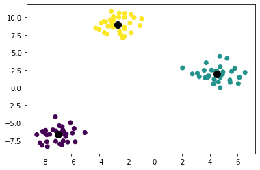
Figure 7.1 – Clustering of multiple samples into definite groups

The preceding figure shows the clustering of multiple samples into three different clusters.

Anomaly detection

This is a type of UL that is mainly used for detecting abnormal or unusual behavior as compared to an established behavior, hence the name anomaly detection. Anything that is deviating from the established baseline behavior is called an anomaly. Among anomaly detection methods, the most important is outlier detection, followed by the novelty detection method.

Outlier detection

Let’s understand what an outlier is first. Outliers are a fraction of samples that differ from the rest of the samples in the population. There are several reasons why this happens—for example, in experimental procedures, those samples are functionally different from the majority of the samples, and so on. In general, exploratory data analysis (EDA) and data processing methods can help remove outliers that arise because of experimental procedures so affect downstream analysis. However, in the latter case, those outliers need to be further analyzed to find the exact reason why they are different from the rest of the samples. In biology and genomics disciplines, outlier detection is very important because it may indicate an important event that is far separated from the rest of the other data points, and so a closer inspection may reveal some interesting insights. For example, a few genes may unusually show higher expression compared to the rest of the genes, which might indicate that these might be relevant to some biological condition.

As can be seen in the following screenshot, running the data with an outlier detection method has discarded several outliers:

Figure 7.2 – Outlier detection before and after removing outliers

The preceding shows how the data looks with outliers (a) and after removing outliers (b).

Novelty detection

In contrast to outlier detection, the original data does not contain any outliers. Here, we are interested in identifying whether a new observation is an outlier, which we refer to as a novelty. Let’s understand this bit further. Consider a dataset of n samples coming from the same distribution. Suppose we add one more observation to that dataset. There are two possibilities—is the new observation so different from the rest of the observations that it is not considered regular (novel) or is the new observation so similar to the other observations that we cannot distinguish it from the other observations? This is where novelty detection methods are useful.

Association

Association is where the algorithm tries to learn new and interesting insights hidden from the training dataset without any labels. The relationship is returned in the form of rules or frequent item sets. The unsupervised algorithm finds certain key attributes (features) of the data sample and tries to predict other attributes with which they are closely associated. One thing to remember with this method is the association rule is a descriptive, not a predictive, method.

Now that we understand what UL approaches are, let’s now dive deep into understanding autoencoders, which are one of the two most popular unsupervised DL approaches that can harness the power of DL without the need for labels in the data.

What are autoencoders?

Autoencoders are a type of deep NN (DNN) that can learn an efficient reduced representation of the data in an unsupervised way and minimize the error between the compressed and subsequently reconstructed data compared to the original data. Why compress the data and then reconstruct the original data? Isn’t it counterintuitive? Suppose you are on your vacation and took pictures, but you realized after you return from vacation that a picture has noise because of dim light. Wouldn't it be nice if there was a way to remove the background and make the picture great? This is, in computer vision lingo, called feature variation, which removes any noise in a picture. This is what autoencoders do. They learn a representation or latent space from the training data to ignore signal noise. The compression step forces the network to only learn the most important latent features. This is because if the model is at full capacity, it will just copy the data without learning any useful features regarding the data structure. During reconstruction, the network ignores the non-essential features and thereby ignores signal noise.

Autoencoders compress the data into a reduced representation of a low-dimensional latent space using multiple non-linear transformations through layers in a DNN. This concept may sound familiar to you because we have a similar method called PCA that does the same thing. So, what’s the difference between the two different methods? Well, the biggest difference between PCA and autoencoders is the type of transformation. Let’s understand it from the following outline:

• PCA is a dimensionality reduction technique (DRT) that converts the input values into a few components that best represent the variance in the data and is mainly a linear transformation method.
• An autoencoder, on the other hand, is a non-linear transformation method that uses a non-linear activation function and multiple NN layers to transform the data and compress it. Autoencoders are more efficient to learn model parameters because they use several layers, unlike PCA, which can learn from one huge transformation. Autoencoders can make use of pre-trained models that were trained and optimized on different datasets (a process termed transfer learning or TL), whereas PCA needs to be run every time on a new dataset.

Note

One thing to note is that the autoencoder doesn’t need to be a fully connected DNN as seen in vanilla NNs but can also be convolutional layers that best work for audio, video, and sequential data.

Autoencoders are quite useful for non-linear transformation, which is a common task in many datasets, such as sequential, image, text, genomics datasets, and so on. Let’s understand some of the properties of autoencoders in the next section.

Properties of autoencoders

The three main properties of autoencoders are 1) they are data-specific, 2) they are lossy, and 3) they learn automatically instead of being manually engineered by humans. Let’s look at this in more detail:

• Autoencoders only work on the data on which they have been trained which means their behavior is data specific
• Compared to the original input, the output from Autoencoders is always degraded and hence it is lossy
• Similar to other DL models, Autoencoders learn features from the data automatically and so there is no need to extract features manually.

How do autoencoders work?

So, why do autoencoders reconstruct the input as an output? Why is it of interest to us, then? The trick is, unlike other supervised NNs that we have seen so far, we do not care about the output here, but what we do care about is the compressed representation (or 'latent space') of the data in the hidden layers. If we reduce the number of neurons in the hidden layers, then the network tries to learn the weights and biases with few neurons in the hidden layers to create a dense representation of data (Figure 7.3). That means the hidden layers in the autoencoder only have to learn the most key features of the input data. For example, if we train an autoencoder on a genome without any mutations (reference genome or gold standard reference), it will learn mutations as something abnormal when used on another genome. This is exactly what an autoencoder does.

You can see a visual representation of Autoencoder in here:

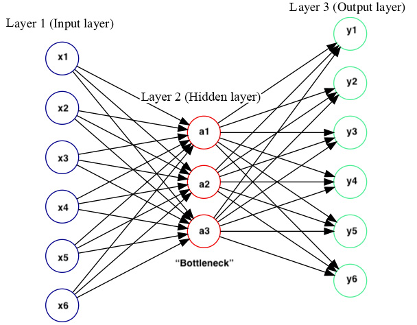
Figure 7.3 – Compressed representation of data

As portrayed in Figure 7.4, we take an unlabeled dataset and convert it to an SL dataset by generating outputs as shown in the output layer, which is reconstructed from the original input. During training, we minimize the reconstruction error, by taking the difference between the original input and the reconstructed output. The output is the same as the input, so we do not need to create labels, hence an autoencoder is good for unlabeled data:

Figure 7.4 – Basic concept of an autoencoder

So, in summary, an autoencoder does three main things:

• Takes the input data
• Compresses the input and learns a representation
• Reconstructs the output without noise and background

That’s it. Now, let us understand the architecture that allows it to do these tasks effectively.

Architecture of autoencoders

The overall goal of autoencoders is to derive an identity function in an unsupervised way so that it can reconstruct the original input through a reduced representation of the input.

Have a look at the following diagram:

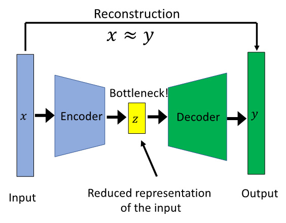
Figure 7.5 – Architecture of an autoencoder

Figure 7.5 shows a typical autoencoder structure where is the input, is the reduced representation of the input, and is the output. The rectangles represent layers in a NN architecture. Autoencoders try to reconstruct the original input, and so the reconstruction is .

So, how does an autoencoder ensure that it reconstructs the original output? Let’s look at the basic architecture of an autoencoder to understand more about it. Leaving out input and the reconstructed output, an autoencoder has three main blocks:

• Encoder: The encoder is the part of the network that is mainly responsible for compressing the input into latent representation.
• Bottleneck: The bottleneck layer or latent or reduced representation layer is a reduced dimension and is the most important attribute of an autoencoder. This hidden layer takes the input data and compresses that within the bottleneck layer. It constrains the amount of information, enabling learned representation of super-complex data in a non-linear way in only a few different dimensions. Without a bottleneck, the network would just simply memorize the input values by passing through the network.
• Decoder: The decoder is the part of the network that is finally responsible for reconstructing the output. It evaluates the representation of the data and provides feedback to the network.

In addition to the preceding three fundamental blocks, other key architectural components of an autoencoder are the loss function and regularization. An autoencoder uses the loss function to compute the error between the original inputs and reconstructed output, and this way, the loss function encourages the model to be sensitive to the inputs. The next term is regularization, which prevents the model from overfitting. Let’s understand how these three blocks work, using a couple of examples.

Image compression

Image compression is a very typical application of an autoencoder. Let’s have a look at this in more detail:

• In this case, for example, if we pass an image of dimensions (32,32,1) to the input layer, we need to flatten the image before we can pass it to the NN architecture.
• A flattened image now becomes 1,024 (32 x 32 = 1,024) and this is then passed to the encoder block. The encoder compresses the input.
• The output from this encoder block is then fed into the bottleneck layer, which consists of 8–16 neurons.
• Next, the decoder block tries to reconstruct the original image from the bottleneck layer, as shown in Figure 7.6.
• If you look at the input and reconstructed output images, they both look the same, so you might be wondering how you would know whether we have successfully reconstructed them or not. This is where we use the loss function, which computes the difference between the input and output images, which can then be minimized as shown in the following figure:

Figure 7.6 – How an autoencoder works for image compression

How can we leverage autoencoders for genomics applications? Now, let’s look at a genomics example. For this, we will use Single-cell RNA sequencing (scRNA-seq), which is a very popular sequencing technology for single-cell sequencing.

scRNA-seq

In the simplest use case, we want the autoencoder to take input data, learn a representation of the data in an unsupervised way, and output the data without noise or reconstruct the input as output. Let’s see an example of how it can be done in genomics. In a scRNA-seq technology, zero counts can arise either because of low mRNA capture rate (dropouts), due to experimental limitations, or because mRNAs are not expressed in that cell type (structural zeros). The main challenge while doing scRNA-seq data analysis is deciding which genes are zero counts due to dropouts versus structural zeros. Several methods exist to address this issue, such as imputation, which relies on correlation structure between the cells and genes to differentiate dropouts from structural zeros. We can treat this as a denoising problem and try to denoise the gene expression data to remove any background noise (dropouts) so that only structural zeros are present.

In the following diagram, we have a typical autoencoder with encoder, bottleneck, and output blocks:

Figure 7.7 – Autoencoders for denoising gene expression data

The input as shown above is a gene expression matrix consisting of cells as columns and genes as rows. In this example, we have five genes, and each gene has expression values from each of the five cell types. The dark-colored boxes indicate zero counts. During the training of an autoencoder, we pass this gene expression matrix in the input layer (five nodes here represent five genes), which are then passed to the Encoder block. The output from the Encoder block is the reduced representation in the bottleneck layer, and finally, the decoder reconstructs the original input from bottleneck layer. The output layer also has a similar number of nodes to the input (five), and it may contain values of the mean of the negative binomial distribution and the final output matrix that shows the denoised expression.

In this way, autoencoders compress the input into low-dimension space and learn the features such as similarities of non-zeros there to decide how to fill in the blanks or denoise the data, as shown in this example.

Types of autoencoders

In general, there are six types of autoencoders. Let’s briefly discuss each of those in the following section.

Vanilla autoencoders

A vanilla autoencoder is also called a complete autoencoder or a standard autoencoder that we have seen before. This is a very simple autoencoder that has three layers—an input layer, a bottleneck layer, and an output layer. Here, the input and output are the same, and reconstruction of the original output is learned using an optimizer such as Adam. We can use some loss functions such as MSE. The input might be an image of size 28 x 28 x 1 pixel, which will be n=784 nodes, and the output will be the same size, so it will be n=784 nodes also. The bottleneck layer can be n=64 nodes, which is smaller than the input size of 784, which will help the autoencoder to learn the compressed representation of the data. By constraining the number of nodes in the bottleneck layer, we can restrict the amount of information that can be passed through the network. The model is trained until the reconstruction loss is minimal. Since there is no regularization term in this type of autoencoder, we must ensure the bottleneck layer has a restricted number of nodes so that the network is not copying the original input into the output layer.

Deep autoencoders

Deep autoencoders, in contrast, have multiple layers in both the encoder and decoder blocks but just have one bottleneck layer. In this type of autoencoder, we use a stack of layers.

Convolutional autoencoders

In Chapter 5, Introducing Convolutional Neural Networks for Genomics, you learned about convolutions and how they are used for image recognition, image classification, transcription factor-binding site detection, and so on. If you remember, we used a fully connected layer before the final output layer in that architecture. We can also use autoencoders instead of fully connected layers in a CNN architecture. During training, the image or one-hot encoded DNA sequence is downsampled using several layers in the CNN such as convolution and pooling layers, and having autoencoders instead of a fully connected layer ensures we learn a compressed image or data. In practice, autoencoders used in image settings are always convolutional autoencoders because they perform much better than the other types of autoencoders for image data.

Regularized autoencoders

So far, we have seen autoencoders that work mainly by placing constraints in the network so that they can learn the useful structure from the data. Instead of putting constraints on the model capacity by keeping the encoder and decoder shallow and the bottleneck layer small, we can impose sparsity in the hidden layers even if the number of hidden units is larger. So, how do we do that in the network? It is mainly done through regularization (such as in SL). There are three different types of regularized autoencoders—sparse autoencoders, contractive autoencoders, and denoising autoencoders.

Sparse autoencoders

A sparse autoencoder is a type of regularized autoencoder that doesn’t put any constraints on the number of nodes in the hidden layer. Instead, it penalizes the activations within a layer. This is different from traditional regularization methods such as Lasso and Ridge where we penalize the weights of the edges. This way, we encourage only a certain number of nodes in the encoder and decoder blocks.

You can see a visual representation of this here:

Figure 7.8 – A simplified sparse autoencoder

As can be seen in Figure 7.8, only a certain number of nodes are activated in the encoder and decoder block, shown by the pale-colored nodes based on the level of their activation.

Contractive autoencoders

These are similar to regularized autoencoders, which we have seen before, except that the learning is done by applying a penalty term to the loss function. It is better than the other two regularization-based autoencoders for feature learning.

Denoising autoencoders

A denoising autoencoder introduces artificial noise (by converting some inputs into zeros) in the data so that the autoencoder doesn’t just copy the data as output without learning any structure of the data. The goal of denoising autoencoders is to recover the undistorted input, as shown in Figure 7.9. In this case, the autoencoder learns an approximation mapping function toward a lower dimension that best describes the natural data without any noise. The loss function tries to reduce the output and the noise input. Denoising autoencoders are a very popular type of autoencoder and are mainly used in image denoising to remove any unwanted noise in images and remove dropouts (non-zeros introduced to a low RNA capture rate) in scRNA-seq data. We have seen an example of this in the previous section:

Figure 7.9 – An example of a denoising Auto encoder

The preceding figure shows an example of denoising autoencoder that takes an input image with noise and produces a cleaned output.

Variational autoencoders

Variational autoencoders (VAEs) are modern types of autoencoders. Both VAE and GANs (which we will learn about in the next chapter) learn a latent variable model from the input data. The main difference between a VAE and other autoencoder types is parameters of a probability distribution of the data. Whereas typical autoencoders are deterministic and try to reduce the error between output and original input (reconstruction error), VAEs, in contrast, are stochastic. Unlike other autoencoders, this is very complex and it is beyond the scope of this chapter to go into the details of a VAE.

Autoencoders for genomics

Several applications of autoencoders for genomics exist. The most common type of application, however, is for predicting gene expression from microarray and RNA-Seq datasets. Let’s understand how autoencoders work for gene expression analysis.

Gene expression

The main application of autoencoders, as you learned in the previous section, is for gene expression analysis, which includes

• Time-series gene expression where they are mainly used at the preprocessing step for clustering, cDNA microarrays
• RNA-Seq, where they are used to predict the organization of transcriptomics machinery
• Gene expression, where they are mainly used for identification of biological signals and patterns respectively

In a typical gene expression experiment, the inputs are typically numerical values estimating how much RNA is produced from a DNA template through transcription across various cells, tissues, or conditions. Let’s look at some popular autoencoder applications for predicting gene expression.

ADAGE

Analysis using Denoising Autoencoders for Gene Expression (ADAGE) (https://www.biorxiv.org/content/10.1101/030650v1) is a popular method for unsupervised gene expression analysis using stacked denoising autoencoders. Briefly, the ADAGE model integrates data without requiring any gene function, gene pathway, or experimental labeling, and so making it a suitable method for any large expression datasets. Briefly, random noise is added to the expression data from various samples. Then, these corrupted expression datasets are processed as inputs to the encoder of the autoencoder NN. The output from the encoder is fed into the bottleneck layer consisting of 30 nodes. The encoder tries to generate the output, and the resulting ADAGE model outputs genomics measurements, which are biological features such as strain, oxygen, and so on.

Learning and representing the hierarchical organization of yeast transcriptomic machinery

In this genomics application, stacked autoencoders are used to learn biological features in yeast from microarray experiments (https://bmcbioinformatics.biomedcentral.com/articles/10.1186/s12859-015-0852-1). The hidden or bottleneck layer that was trained from these autoencoders is then used to encode biological representations in yeast.

Boosting gene expression clustering

Autoencoders are currently used to cluster gene expression profiles as a powerful tool for inferring information from unsupervised data such as gene expression profiles (https://www.biorxiv.org/content/early/2017/11/05/214122).

Use case – Predicting gene expression from TCGA pan-cancer RNA-Seq data using denoising autoencoders

Gene expression analysis is a typical use case in the genomics domain. Gene expression can reveal a lot of biological insights about the state of the cell, tissue, or condition. Currently, a lot of techniques, both traditional and non-traditional, are available for gene expression predictions. Autoencoders, because of their ability to reconstruct data, were proven successful previously to extract novel biological insights from gene expression data. With that goal in mind, in this current use case, we will train an autoencoder from The Cancer Genome Atlas (TCGA) pan-cancer RNA-Seq data.

Data collection

TGCA consists of several genomics measurements from several tumors across different cancer types. Among them, gene expression measurements can capture information about the biological state of each tumor and is great dataset for our purposes. For this use case, we will train and evaluate an autoencoder network from this data consisting of the 5,000 most variably expressed genes from 10,459 samples. This whole dataset is referred to as pan-cancer data. The data was downloaded from https://github.com/greenelab/tybalt/blob/master/data/pancan_scaled_zeroone_rnaseq.tsv.gz.

Data preprocessing

The pan-cancer data is already preprocessed and batch-corrected, so there is no need to do any further data preparation. In addition, the variability of gene expression was calculated by median absolute deviation (MAD).

Model selection

For this use case, we will select an denoising autoencoder that accepts the 5,000 genes as input reduced representation of 100 features, and reconstruct to the original 5,000 genes.

Model training

Let’s start training a denoising autoencoder. This phase can be divided into multiple sub-phases, which we will see in the following sections. Follow the next steps:

1. Start by importing the libraries first:

   import os

   import numpy as np

   import pandas as pd

   import matplotlib.pyplot as plt

   import seaborn as sns

   from keras.layers import Dense

   from keras.models import Sequential

   from sklearn.model_selection import train_test_split

Here, we are importing all dependencies (libraries and packages) that are needed for autoencoders. We use Keras for creating an autoencoder NN. To do this, we will import the Sequential API, which will allow us to build the network easily.

2. Next, we will import the TCGA RNA-Seq data that we discussed previously:

   pancan_rnaseq_df = pd.read_csv(pancan_scaled_zeroone_rnaseq.tsv, index_col=0, sep=" ", low_memory=False)

   pancan_rnaseq_df.iloc[:2,:5].head()

After we download the data from the TCGA portal, we import that data into the workspace using pandas’ read_csv function and print the first two rows and five columns. The following table shows the first two rows and five columns of the pancan RNA-Seq datasets. Each row corresponds to the sample name and each column corresponds to each gene and its expression in that sample:

	RPS4Y1	XIST	KRT5	AGR2	CEACAM5
TCGA-02-0047-01	0.678296	0.289910	0.034230	0.0	0.0
TCGA-02-0055-01	0.200633	0.654917	0.181993	0.0	0.0

Figure 7.10 – First two rows and five columns of the pancan RNA-Seq datasets

3. Train-test split: By now, you are familiar with this concept. Just to refresh your memory, we need to split the full dataset into training and test datasets. The training dataset will be used for training and validating the model, and the test dataset will be used for model evaluation:

   pancan_rnaseq_df_train, pancan_rnaseq_df_test = train_test_split(pancan_rnaseq_df, test_size=0.1, shuffle=True)

   pancan_rnaseq_df_train.shape, pancan_rnaseq_df_test.shape

   ((9413, 5000), (1046, 5000))

Here, we are splitting the data in the ratio of 90:10 train:test. The final data dimensions are also printed to confirm that the data was split properly.

4. Defining the layers of the autoencoder: Next, we will define the layers of our autoencoder NN. For this, we will use the Sequential API of Keras, which is simpler but less flexible compared to the Functional API that you have learned before. The code is illustrated here:

   # This is the size of our encoded representations

   encoding_dim = 100

   numb_of_features = pancan_rnaseq_df.shape[1]

   # Defining the 'Autoencoder' full model

   autoencoder = Sequential()

   autoencoder.add(Dense(encoding_dim, activation="relu", input_shape=(numb_of_features, )))

   autoencoder.add(Dense(numb_of_features, activation="sigmoid"))

   autoencoder.summary()

   Model: "Autoencoder" _________________________________________________________________

   Layer (type) Output Shape Param # =================================================================

   dense_6 (Dense) (None, 100) 500100

   dense_7 (Dense) (None, 5000) 505000 =================================================================

   Total params: 1,005,100

   Trainable params: 1,005,100

   Non-trainable params: 0

This is a lot of code. Let’s try to break this down:

1. First, we define the encoding layer dimensions (bottleneck layer) with encoding_dim and the number of features (which is the same as the number of columns in the dataset) with numb_of_features.
2. Next, we define the autoencoder in full:

1. For this, first, we assign a new instance of the Sequential model type to a variable called autoencoder.
2. Next, we add a densely connected layer that has encoded_dim or the number of neurons corresponding to the learned representation of the model, a 'reLu' activation function, and an input_shape parameter. Unlike the Functional API that you have learned in Chapter 4, Deep Learning for Genomics, there is no need to define the input layer here as the input layer is defined under the hood.
3. Finally, we add another densely connected layer that accepts the learned representations from the encoding_dim parameter, converts them back into numb_of_features, and is referred to as a decoder block. This has sigmoid as an activation function.

5. Compile the autoencoder to prepare for training: We should compile the model first before we can train the model. Keras’ Sequential API makes this very easy for us. With a single line of code, you will be able to compile the model, as shown here:

   autoencoder.compile(optimizer="adam", loss='mse')

Here, we have taken the autoencoder model and added an Adam optimizer, which is a very popular algorithm for optimizing models, and added MSE as the loss function for us to understand the level of reconstruction that happened during model training.

6. Fit the model: Now, we are ready to fit and train the model with the compiled model from the previous step. Again, this is very easy to do in Keras:

   hist = autoencoder.fit(np.array(pancan_rnaseq_df_train), np.array(pancan_rnaseq_df_train), shuffle=True, epochs=10, batch_size=50, validation_split=0.2)

Here, we feed pancan_ranseq_df_train both as features and targets. The other parameters included here are epochs and batch_size, which are hyperparameters that you can tune (you will learn more about this in Chapter 11, Model Deployment and Monitoring). For this example, we will use 10 epochs and a batch size of 50. Finally, to prevent overfitting the model during training, we ask it to use 20% of training data as validation data for cross-validation purposes.

7. Visualize training performance: Let’s quickly visualize how the model performed after training. For this, we will compare the training loss with the validation loss:

   history_df = pd.DataFrame(hist.history)

   ax = history_df.plot()

   ax.set_xlabel('Epochs')

   ax.set_ylabel('Reconstruction Loss')

This will generate a reconstruction loss like the one shown next. loss here indicates the training loss and val_loss indicates the validation loss. As expected, with more epochs, the training loss goes down, and similarly, the validation loss is shown to be going down, which indicates the model is not overfitting:

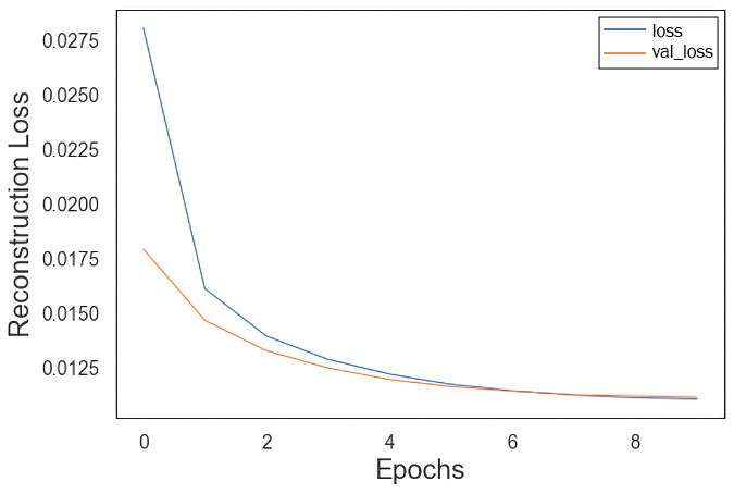
Figure 7.11 – Reconstruction loss visualized

Note

Please note that we only have 10 epochs for this training, and with more epochs and other hyperparameter optimization, this model loss will be even lower. But this is a good starting point.

8. Model predictions and calculations of reconstruction loss: Before we accept this model, we should check to see how well the model has done concerning reconstruction. You can do this in Keras very simply by running the following commands:

   reconstruction = autoencoder.predict([input_sample])

   reconstruction

   array([[0.7896689 , 0.10001165, 0.5899597 , ..., 0.08822288, 0.32368636, 0.51022756]], dtype=float32)

The output here indicates the difference in the gene expression values between the original input and the reconstructed output. This is just one example, but you can imagine predicting the reconstruction loss for the whole dataset and looking at the average reconstruction loss for all the genes in the DataFrame. You can also look at the most and least activated nodes from the predictions and, most importantly, plot the distribution for all 100 encoded features.

Summary

The application of unsupervised DL through learned representation is becoming extremely popular in genomics because of the large-scale datasets produced using NGS technologies. Autoencoders are being routinely used by researchers because of their promise and success across many genomics applications. Autoencoders learn by the reduced representation of the data through compression and reconstruction. During the process, they learn the key features of the data and identify the data structure automatically from examples rather than through handcrafting by humans. Diverse types of autoencoders exist to ensure that the reduced representation of the data identifies the key attributes of the original data. Autoencoders have several applications in genomics, mainly in gene expression analysis. With tools such as ADAGE, autoencoders are helping genomics datasets with no labels get biological insights from that data. We started the chapter by understanding what is unsupervised learning and the different algorithms that are currently available for unsupervised learning. We learned that Autoencoders is how they learn the key features of the data and identify the data structure automatically from examples rather than through handcrafting by humans. We then looked at the unique architecture of Autoencoders that enable us to learn these reduced representations and help address the challenging problems in genomics such as gene expression, denoising, and so on. Autoencoders have different types depending on the applications and we have a few examples such as denoising autoencoders and sparse autoencoders. Toward the end of the chapter, we took a publicly available dataset and build an Autoencoder model to predict gene expression with few lines of code.

One of the main limitations of autoencoders is that if there is no structure in the data—for example, if each data point is independent of the other in the input data—autoencoders will fail. If there is a correlation in the input features, then autoencoders will work. This is because autoencoders learn how to compress the data based on key attributes—for example, the correlation of the input features identified during the training process. Another limitation is that autoencoders can only work on the data that they have been trained on. That means they will only be able to compress the data similar to the data that they have been trained on. Despite these limitations, autoencoders have been widely used in many genomics applications, ranging from denoising scRNA-seq, time-series gene expression, identification of biological patterns, dimensionality reduction for data visualization, and so on.

We will look at the GAN generative model NN architecture in the next chapter.