2

Genomics Data Analysis

Genomics gained mainstream attention when the Human Genome Project published the complete sequence of the human genome in 2003. Over the last decade, genomics has become the backbone of drug discovery, targeted therapeutics, disease diagnosis, and precision medicine, leading to the chances of successful clinical trials. For example, in 2021, over 33% of FDA-approved new drug approvals were personalized medicines, a trend that sustained for the past five years (https://www.foley.com/en/insights/publications/2022/03/personalized-medicine-2021-fda-guideposts-progress). This growing use of genomics can be mainly attributed to the drastic decrease in the cost and turnaround time of DNA sequencing. For instance, while human genome sequencing was reported to cost around $3 billion and took 13 years to complete, today, you can get your genome sequenced in a day with less than $200 (https://www.medtechdive.com/news/illumina-ushers-in-200-genome-with-the-launch-of-new-sequencers/633133/). Because of this incredible success of the genomics industry, more and more research professionals and scientists are now routinely generating genomic data than ever before to understand how genome functions affect human health and disease. It is estimated that over 100 million genomes will be sequenced by 2025 (https://www.biorxiv.org/content/10.1101/203554v1) and with the right data analysis and interpretation of this massive data, this information could pave the way to a new golden age of precision medicine.

To find and interpret biological information hidden within this data, it is important to have a solid foundation of genomics data analysis methods and algorithms. The objective of this chapter is to provide fundamentals of genomics data analysis using Biopython, which is one of the most popular Python modules that provides a suite of new commands for working with sequence data. Using Biopython, you can make sense of the vast amounts of available genomics data and extract biological insights. If you are a genomic scientist or a researcher working in the area of genome biology, or someone familiar with these concepts, then please free to skip this chapter or quickly skim through it for a quick refresh. By the end of this chapter, you will know the fundamentals of genomics, genome sequencing, and genome data analysis, how to use the Biopython module of Python for genomics data analysis, and prepare the data in such a way that is compatible with machine learning (ML).

As such, the following topics are covered in this chapter:

• What is a genome?
• Genome sequencing
• Analysis of genomic data
• Introduction to Biopython for genomic data analysis

Technical requirements

This course assumes that you have a basic knowledge of Python for programming, so we will not introduce Python in this book.

Note

For a quick refresher on Python fundamentals, please refer to https://www.freecodecamp.org/news/python-fundamentals-for-data-science/.

Instead, you will be introduced to Biopython, which is a powerful library in Python that has tools for computational molecular biology for performing genomics data analysis.

Installing Biopython

Installing Biopython is very easy, and it will not take more than a few minutes on any operating system.

Step 1 – Verifying Python installation

Before we install Biopython, first check to see whether Python is installed using the following command in your command prompt:

$ python --version
Python 3.7.4

Note

The $ character represents the command prompt.

If your command prompt returns something like this, then it shows that Python is installed and 3.7.4 is your version of Python on your computer.

Note

Biopython only works with Python version 2.5 and above. If your Python version is <2.5, you should upgrade your Python version.

Alternatively, if you get an error like this, then you should download the latest version of Python from https://www.python.org/downloads/, install it, and then run the preceding command again:

-bash: python: command not found

Step 2 – Installing Biopython using pip

The easiest way to install Biopython is through the pip package manager, and the command to install is as follows:

$ pip install Biopython==1.79

Collecting Biopython

  Using cached https://files.pythonhosted.org/packages/4a/28/19014d35446bb00b6783f098eb86f24440b9c099b1f1ded3 3814f48afbea/Biopython-1.79-cp37-cp37m-macosx_10_9_x86_64.whl

Collecting numpy (from Biopython)

  Downloading https://files.pythonhosted.org/packages/09/8c/ae037b8643aaa405b666c167f48550c1ce6b7c589fe5540de6d83e5931ca/numpy-1.21.5-cp37-cp37m-macosx_10_9_x86_64.whl (16.9MB)

    100% |████████████████████████████████| 16.9MB 3.4MB/s

Installing collected packages: numpy, Biopython

Successfully installed Biopython-1.79 NumPy-1.21.5

The preceding response indicates that Biopython version 1.79 is successfully installed on your computer.

If you have an older version of Biopython, try running the following command to update the Biopython version:

$ pip install Biopython –upgrade

Requirement already up-to-date: Biopython in python3.7/site-packages (1.79)

Requirement already satisfied, skipping upgrade: numpy in python3.7/site-packages (from Biopython) (1.21.5)

The preceding message indicates that Biopython is the latest version that you have on your computer. If your Biopython version is older than the most recently updated one of Biopython, then the old version of Biopython and NumPy (a dependency for Biopython) will be replaced by the new version.

Step 3 – Verifying Biopython installation

After you have successfully installed Biopython, you can verify Biopython installation on your machine by running the following command in your Python console:

$ python3.7

Python 3.7.4 (default, Aug 13 2019, 15:17:50)

[Clang 4.0.1 (tags/RELEASE_401/final)] :: Anaconda, Inc. on darwin

Type "help", "copyright", "credits" or "license" for more information.

>>> import Bio

>>> print(Bio.__version__)

1.79

Note

>>> here represents the Python prompt where you would enter code expressions. Please note the underscores before and after the version. You can exit the console by using the exit() command or pressing Ctrl + D (which works in Linux and macOS only).

The preceding output shows the version of Biopython, which, in this case, is 1.79. If that command fails, your Biopython version is very out of date and you should upgrade it to the new version as indicated before.

There are alternate ways of installing Biopython, such as installing from the source, and you will find more information on it here: https://biopython.org/wiki/Packages

Matplotlib

We will be using Matplotlib, a very popular Python library for visualization. It is one of the easiest libraries to install and use. To install Matplotlib, simply run pip install matplotlib in your terminal. Then, you can include import matplotlib.pyplot as plt in your Python script, which you will see later in the hands-on section of this chapter.

What is a genome?

Before we discuss genomes, let’s do a quick Genetics 101. A cell represents the fundamental structural and functional unit of life. DNA contains the instructions that are needed to perform different activities of the cell. DNA is the basis of genetic studies and consists of four building blocks called nucleotides – adenine (A), guanine (G), cytosine (C), and thymine (T), which store information about life. The sequence of DNA is a string of these building blocks, also referred to as bases. DNA has a double-helix structure with two complementary polymers interlaced with each other. In the complementary strand of DNA, A matches with T, and G matches with C, to form base pairs.

A genome represents the full DNA sequence of a cell that contains all the hereditary information. The genome consists of information that is needed to build and maintain the whole living organism. The size of genomes is different from species to species. For example, the human genome is made up of 3 billion base pairs spread across 46 chromosomes, whereas the bread wheat genome consists of 42 chromosomes and ~ 17 gigabases. A region of a genome that transcribes into a functional RNA molecule, or transcribes into an RNA and then encodes a functional protein, is called a gene. This is the simplest of definitions, and there are several definitions of a gene, but overall, a gene constitutes the fundamental unit of heredity of a living organism. By analogy, you can imagine the four nucleotides (A, G, C, and T) that make up the gene as letters in a sentence, genes as sentences in a book, and the genome as the actual book consisting of tens of thousands of words.

Genome sequencing

After the discovery of the DNA structure, scientists were curious to determine the exact sequence of DNA (aka interpreting the whole book). A lot of pioneering discoveries paved the way for the sequencing of DNA, starting with Walter Gilbert when he published the first nucleotide sequence of the DNA lac operator consisting of 24 base pairs in 1973 (https://www.ncbi.nlm.nih.gov/pmc/articles/PMC427284). This was followed by Frederick Sanger who for the first time sequenced the complete DNA genome of the phi X174 bacteriophage (https://pubmed.ncbi.nlm.nih.gov/731693/). Sanger pioneered the first-ever sequencing of genes through the method of DNA sequencing with chain-terminating inhibitors. In the last 50 years, available sequencing technologies have been restricted to relatively small genomes, but advances in DNA sequencing technologies such as next-generation sequencing (NGS) have revolutionized genome sequencing because of their cost, speed, throughput, and accuracy. As more and more genomes are sequenced, this extended knowledge can be utilized for the development of personalized medicines to prevent, diagnose, and treat diseases and, ultimately, support clinical decision-making and healthcare. It’s beyond the scope of this chapter to go into the historical background of DNA sequencing technologies. Here, we will briefly present the different DNA sequencing technologies that have led to major milestones in genome sequencing.

Sanger sequencing of nucleic acids

Sanger sequencing, also known as the “chain termination method” is the first-generation sequencing method, and was developed by Frederick Sanger and his colleagues in 1977 (https://www.ncbi.nlm.nih.gov/pmc/articles/PMC431765/). It was used by the Human Genome Project to sequence the first draft of the human genome. This method relies on the natural method of DNA replication. Sanger sequencing involves the random incorporation of bases called deoxyribonucleoside triphosphates (dNTPs) by DNA polymerase into strands during copying, resulting in the termination of invitro transcription. These bases in the short fragments are then read out based on the presence of a dye molecule attached to the special bases at the end of each fragment. Despite being replaced by NGS technologies, Sanger sequencing remains the gold standard sequencing method and is routinely being used by research labs throughout the world for quick verification of short sequences generated by polymerase chain reaction (PCR) and other methods.

Evolution of next-generation sequencing

Next-generation sequencing first became available at the start of the 21st century and it completely transformed biological sciences, allowing any research lab to perform sequencing for a wide variety of applications and study biological systems at a level unimaginable before. NGS aims to determine the order of nucleotides in the entire genome or targeted regions of DNA or RNA in a high-throughput and massively parallel manner. The biggest advance that NGS offered compared to traditional Sanger sequencing and other approaches is the ability to produce ultra-high-throughput genomic data at a scale and speed. NGS technologies can be broadly divided into second-generation sequencing and third-generation sequencing technologies, depending on the type of sequencing methodology.

Second-generation DNA sequencing technologies

Alongside the developments in large-scale dideoxy-sequencing efforts, another sequencing technology that emerged in the last 15 years that revolutionized DNA sequencing is the NGS technology. There are a lot of technologies under NGS starting with pyrosequencing, by 454 Life Sciences, but the most important of all of them are bridge amplification technologies that were brought forth by Solexa, which was later acquired by Illumina. In contrast to Sanger sequencing, Illumina leverages sequencing by synthesis (SBS) technology, which is the tracking of labeled nucleotides as the DNA is copied in a massively parallel fashion generating output ranging from 300 kilobases up to several terabases in a single run. The typical size fragments generated by Illumina are in the range of 50-300 bases. Illumina dominates the NGS market.

Third-generation DNA sequencing technologies

These technologies are capable of sequencing single DNA molecules full length without amplification, and they allow the production of sequences (also called as reads) much longer than second-generation sequencing technologies such as Illumina. Pacific Bioscience and Oxford Nanopore Technologies dominate this sector with their systems called single-molecule sequencing real-time (SMRT) sequencing and nanopore sequencing, respectively. Each of these technologies can rapidly generate very long reads of up to 15,000 bases long from single molecules of DNA and RNA.

Analysis of genomic data

Genomic data analysis aims to provide biological interpretation and insights from genomics data and help drive innovation. It is like any other data analysis with the exception that it requires domain-specific knowledge and tools. With the advances in NGS technologies, it is estimated that genomic research will generate significant amounts of data in the next decade. However, our ability to mine insights from this big data is lagging behind the pace at which the current data is being generated. As new and more high-throughput genomic data is getting generated, data analysis capabilities are sought-after features for researchers and other scientific professionals in both academia and industry.

Steps in genomics data analysis

Genomics data is generally complex in nature and size. Researchers are currently facing an exciting yet challenging time with this available data that needs to be analyzed and understood. Analyzing this big genomics data can be extremely challenging. A natural course of action can be ML, which is fast becoming the go-to method for analyzing this data to mine biological insights. We will discuss the application of ML for genomics data in the next chapter but for now, let’s understand the different steps involved in the analysis of genomics data. The main aim of genomics data analysis is to do a biological interpretation of large volumes of raw genomics data. It is very similar to any other kind of data analysis but in this case, it often requires domain-specific knowledge and tools. Here, we will discuss data analysis steps for analyzing genomics data. Typical analysis of genomic data consists of multiple interdependent extract, transform, and load (ETL) that transform raw genomic data from sequencing machines into more meaningful downstream data used by researchers and clinicians.

A typical genomics data analysis workflow consists of the following steps: data collection, data cleaning, data processing, exploratory data analysis (EDA), modeling, visualization, and reporting. You might have seen several versions of this workflow but ultimately, a typical genomic data analysis workflow boils down to these five main steps – raw data collection, transforming the data, Exploratory Data Analysis (EDA), modeling (statistical or machine learning), and biological interpretation, as shown in Figure 2.1:

Figure 2.1 – Steps in a typical genomic data analysis workflow

Even though the steps in the genomic data analysis are linear, there are instances when you go back and repeat many of these steps to answer some questions related to data quality or add new datasets in the analysis or optimize the parameters.

Data collection

Data collection refers to any source, experiment, or survey that provides raw data. The genomic data analysis starts right after the experimentation stage, where data is generated if no data is available or if the question cannot be solved with available data. Many times, you don’t need to generate the data and instead can use publicly available datasets and specialized databases. The type and amount of data that needs to be collected are entirely dependent on the questions along with the technical and biological variability of the experimental system under study.

Data transformation

Data transformation consists of converting raw data into data that can be used for downstream analysis, such as EDA and modeling. It consists of quality control and data processing.

Quality control and cleaning

The quality control and cleaning step aims to identify the quality issues in the data and clean them from the raw dataset, generating high-quality data for modeling purposes. Quite frequently, the analysis starts with the raw genomics data (processed data if you are lucky), and it’s mostly messy data. Like any other raw data, genomic data consists of missing values, outliers, invalid, and other noisy data. Since it is a well-known fact that the quality of the output is determined by the quality of the input (garbage in, garbage out), it is super important to subject the data to quality control and cleaning before using it for downstream analysis.

Data processing

The goal of data processing is to convert raw data into a format that is amenable to visualization or EDA or modeling. The data processing step starts after the raw data was collected and cleaned. Briefly, the data processing steps include the following:

• Data munging, which is transforming data from one format to another format
• Data transformation, which includes either normalizing the data or log transformation of the data
• Data filtering, which is a key step to remove data points that have unreliable measurements or missing values.

Exploratory data analysis

EDA is the most crucial step of any data analysis. The goal of EDA is to use various statistics and visualization methods on either the processed or semi-processed data to find the relationships between the variables in the input data, or between samples or correlations between input and output, or detect outliers from the data, and so on. Some examples of EDA include nucleotide composition, di-nucleotide frequencies, guanine-cytosine (GC) content, amino-acid frequencies, and so on.

Modeling

Post-EDA, you might be interested in building a model to get the outcome or get some biological insights from the processed data. Modeling is the process of mapping the relationship between input variables and output. For example, modeling to predict the disease status of a patient either diseased or not from the genomic data such as gene expression, variants detected, and so on. This is called predictive modeling and we will discuss the different algorithms for performing predictive modeling in genomics in the next chapter. As you can see from Figure 2.1, there is also statistical modeling where we can use statistical methods. An example of statistical modeling in genomics is differential gene expression analysis where we are interested to find whether a gene or set of genes is significantly different between datasets, for example, non-diseased versus diseased patients.

Visualization and reporting

Visualization is not a standalone step but is necessary for all the preceding steps. It is visualizing the data using visualization tools before and after each step of the workflow to make informed decisions. Reporting is compiling all the preceding information through plots, tables, and descriptions that describe the complete data analysis. In genomics, there are innumerable visualization and reporting methods developed, and we will use some of them for genomic data analysis later in the hands-on section of this chapter.

Cloud computing for genomics data analysis

The incredible success of NGS technologies with their ability to generate large volumes of data at a low cost and speed has created several challenges in terms of the acquisition, storage, distribution, and data analysis. For example, just a single human genome sequencing run produces approximately 200 GB of raw data and an additional 100 GB of data per genome after data analysis. If we were to manage to sequence 100 million genomes by 2025, then we will accumulate over 200 Exabyte of raw data. In addition to genomics data storage, the data analysis and interpretation of this massive amount of data are incredibly challenging because of the high-throughput computing needed to process this data. This is where cloud computing technologies can aid genomics. Cloud computing has completely transformed the way we run computing in various domains of life sciences. Cloud computing can transform the existing small or on-premises genomic data analysis into efficient genomics data analysis systems on the cloud. They offer solutions for research professionals who currently lack the tools to make full use of this data. The demand for cloud-based solutions for genomics was evident in the last several years, with several big players coming and supporting genomics, such as Amazon Web Services (AWS), Azure, and Google Cloud Platform (GCP). Even though cloud computing provides the resources for computation, they are still expensive and require a credit card to register to use its services. So, to address that, we will either run the analysis on laptops or use free open-source computing platforms such as Google colabs (which you will learn about in future chapters). For this chapter though we will run the analysis on our computers.

Introduction to Biopython for genomic data analysis

In this section, you will be familiarized with the basics of Biopython, and in the subsequent section, you will use Biopython for solving a real-world research question in genomics.

What is Biopython?

Biopython is a popular Python package developed by Chapman and Chang, mainly intended for biological researchers and data miners to analyze genomic data. It was written mainly in Python but also has support for C code to optimize complex computations. It can be run on any operating system (Windows, Linux, and macOS). Biopython provides lots of functionalities to support genomic data and it makes it easy to use Python for genomic data analysis through reusable modules and classes. In addition to providing basic and advanced genomic functionalities, it also has support for parsers for various popular bioinformatics file formats such as BLAST, ClustalW, FASTA, and GenBank, as well as support online databases and servers such as NCBI, Expasy, and so on.

Quick start of Biopython

Before we dive deep into genomics use cases, let’s have a quick introduction to Biopython. If you are already familiar with Biopython basics, please feel free to skip this section and jump into the hands-on section.

Working with sequences

As genomics is the field of sequences, you cannot get away without using them. A sequence is a series of letters, for example, A, G, C, and T string together in DNA, or A, G, C, and U string together in RNA, or amino acids D, T, S, E, P, G, A, C, V, M, I, L, Y, F, H, K, R, W, Q, and N string together in a protein. Let’s look at how Biopython deals with sequence data but before that, let’s refresh your Python knowledge briefly.

Note

An object is defined as a collection of data (variables) and the methods (functions) that define and act on that data. In Python, everything is an object.

Seq object

The first and the most important object to deal with sequence data in Biopython is the Seq object. It essentially combines a Python string with biological methods such as DNA, RNA, or protein.

For example, you can create a Seq object in Biopython for a DNA sequence consisting of letters such as 'AGTAGGACAGAT', as follows:

>>> from Bio.Seq import Seq

>>> my_seq = Seq("AGTAGGACAGAT")

>>> my_seq

Seq('AGTAGGACAGAT')

>>> print(my_seq)

AGTAGGACAGAT

You may be wondering how the Seq object that you created in the preceding code is different from the regular Python string object since they look the same. Well, it differs from the Python string in the kinds of methods it supports. For example, the regular Python string method does not support complement and reverse_complement functions, whereas the Biopython Seq object supports those two along with several other very useful methods. Some of the popular methods for Seq objects include complement and reverse_complement, as shown in the following code block:

>>> my_seq.complement()

Seq('TCATCCTGTCTA')

>>> my_seq.reverse_complement()

Seq('ATCTGTCCTACT')

As you can see from the preceding code block, the Biopython Seq object is very convenient to apply these methods without you writing a function.

Each Seq object has two important attributes:

• Data – The actual sequence string ('ATCTGTCCTACT').
• Alphabet – The type of sequence, for example, DNA, RNA, or protein. By default, it doesn’t represent any sequence. That means Biopython doesn’t necessarily know whether the input to the Seq object is a nucleotide (A, G, C, or T) or protein sequence consisting of the amino acids alanine (A), cysteine (C), glycine (G), and threonine (T). So, keep this in mind when you call methods such as complement and reverse_complement, depending on the type of input sequence.

The Seq object supports two types of methods – general methods (find, count, and so on) and nucleotide methods (complement, reverse_complement, transcribe, back_transcribe, translate, and so on). We will use a few of these methods later in the chapter.

SeqRecord object

After the Seq object, the next most important object in Biopython is SeqRecord or sequence record. This object differs from the Seq object in that it holds a sequence (as a Seq object) with additional information such as identifier, name, and description. You can use the Bio.SeqIO module with the SeqRecord object in Biopython.

SeqIO object

The SeqIO object in Biopython provides the standard sequence input/output interface. It supports several file formats as input and output. The following table (Figure 2.2) lists the selected file formats that the Bio.SeqIO module can read, write, and index. For a full list of file formats, please refer to Biopython’s documentation (https://biopython.org/wiki/Documentation).

Figure 2.2 – List of popular file formats that are supported in Biopython

The main function in the SeqIO object is parse, which accepts either a file handle or a filename along with a format name. It then returns a SeqRecord iterator. Let’s see the parse function in action using FASTA and GenBank file formats now.

FASTA

If you are a genomic researcher, then there is a very high chance that you have used the FASTA format before or at least heard about it. Let’s use the Bio.SeqIO module’s parse function on an example FASTA file.

But first, let’s import the SeqIO model into the Python console:

>>> from Bio import SeqIO

The parse() method takes two arguments – the file handle and the file format. In this example, we will provide the file handle as fh_in and the file format as fasta:

>>> with open("example.fasta") as fh_in:

...     for record in SeqIO.parse(fh_in, "fasta"):

...             print(record.id)

This returns an iterable object, record, with SeqRecord on every iteration, which provides a lot of sophisticated and easy methods. We will see this in action in the sample use case section coming up.

GenBank

Unlike the FASTA format, GenBank is a sequence format that has rich information about gene sequences and includes several fields for various kinds of annotation. The only difference between this file format compared to the FASTA file format while loading into the parse function is to change the format option in the parse method:

>>> with open("example.gbk") as fh_in:

...     for record in SeqIO.parse(fh_in, "genbank"):

...             print(record.annotations)

As shown, we changed the formation from "fasta" to "GenBank" while parsing a GenBank format file.

We will see an example of this in the sample use cases section.

Genomic data analysis use case – Sequence analysis of Covid-19

Now that you have gained some basic knowledge of Biopython and how it can be used on sequence data of various file formats, let’s use this knowledge in a real-world research problem specifically related to sequence analysis. The goal here is to introduce Biopython with the genomic context in the background. The sample use case listed here is to analyze genomic data of Covid-19 with Biopython. We believe tailoring material to the context of genomics makes a difference when learning Biopython for the sake of analyzing genomic data.

Sequence analysis is considered an important part of genomic data analysis. An example of sequence analysis includes inferring sequence composition, calculating GC content, calculation of % T, % A, and so on. In addition, more complicated tasks such as motif searching are also part of sequence analysis. These are considered features derived from sequences for training models, which we will see in the next chapter. These features have a direct impact on prediction purposes during model training. So, it is important to understand how to extract these features from sequence data, and for that, we will use Biopython. For this example, we will use SARS-CoV-2, which is a causative agent for Covid-19 and needs no introduction because of the widespread destruction it caused across the whole world causing millions of deaths:

1. The full sequence of the Wuhan virus can be downloaded (https://www.ncbi.nlm.nih.gov/nuccore/NC_045512.2?report=fasta); save it as covid19.fasta locally on your computer. You can open this FASTA file in a text editor of your choice, and this is how it looks:

Figure 2.3 – Wuhan genome sequence (only a fraction of the sequence is shown here)

Looking at the sequence, you might be wondering why I can’t just use Python for parsing this FASTA file and do sequence data analysis such as calculating GC content, calculation of % T, % A , and so on. Well, you can certainly do that, but as discussed previously, Biopython already has objects and methods suited for this kind of sequence data analysis, and so we will take advantage of that.

2. Let’s create a simple Python script (covid19_meta.py) to parse this FASTA file and run some basic sequence analysis:

   from Bio import SeqIO

   with open("covid19.fasta") as fh_in:

       for record in SeqIO.parse(fh_in, "fasta"):

               print(f'sequence information: {record}')

               print(f'sequence length: {len(record)}')

3. Now, you can execute this script by running it as follows at the command prompt in your terminal:

   $ python3.7 covid19_meta.py

   The preceding command will generate the following output in the terminal:

   sequence information: ID: NC_045512.2

   Name: NC_045512.2

   Description: NC_045512.2 Severe acute respiratory syndrome coronavirus 2 isolate Wuhan-Hu-1, complete genome

   Number of features: 0

   Seq('ATTAAAGGTTTATACCTTCCCAGGTAACAAACCAACCAACTTTCGATCTCTT GT...AAA')

   sequence length: 29903

Note:

Make sure you run this script in the same directory as the covid19.fasta file you saved in Step 1.

Now, let’s try the same code in the Python console:

1. First import all the relevant libraries:

   >>> from Bio import SeqIO

2. Then, run the following code block:

   >>> with open("covid19.fasta") as fh_in:

   ...     for record in SeqIO.parse(fh_in, "fasta"):

   ...             print(f'sequence information: {record}')

   ...             print(f'sequence length: {len(record)}')

   ...

   sequence information: ID: NC_045512.2

   Name: NC_045512.2

   Description: NC_045512.2 Severe acute respiratory syndrome coronavirus 2 isolate Wuhan-Hu-1, complete genome

   Number of features: 0

   Seq('ATTAAAGGTTTATACCTTCCCAGGTAACAAACCAACCAACTTTCGATCTCTT GT...AAA')

   sequence length: 29903

Note

When you run these commands in the console, make sure you do not include >>>.

So, what’s happening here?

1. First, we have loaded the SeqIO module from Biopython.
2. Next, we opened the covid19.fasta file, as we learned about earlier with the parse method.
3. Finally, we printed some basic information about the sequence such as the name, description, number of features, sequence, and sequence length.

What is the length of SARS-COV-2 in kilobases then? Alright, now you know how to read a FASTA file using Biopython. Let’s continue using this FASTA file to perform some basic genomic data analysis.

Calculating GC content

GC content is one of the important features of a DNA sequence as it is an important predictor of gene function and species ecology. GC content is calculated by counting the number of Gs and Cs in the sequence and dividing that by the total sequence length.

However, we don’t need to write a function to calculate GC; thanks to Biopython, we can load the Bio.SeqUtils module and then import the GC function as shown in the following code.

Write a script to calculate the nucleotide percentages as follows:

# Covid19_meta1.py
from Bio import SeqIO
from Bio.SeqUtils import GC
with open("covid19.fasta") as fh_in:
	for record in SeqIO.parse(fh_in, "fasta"):
		print(f'GC content: {GC(record.seq)}')}')
$ python3.7 covid19_meta1.py
GC content: 37.97277865097148

How can you round the value of GC content to two decimals in Python? The result here shows that the covid19 sequence has a GC content of ~38. If you are a genomic researcher, then the GC content of covid19 might look very low to you and in fact, you are right. SARS-CoV-2 has an extremely low GC content compared to other coronavirus species. Why does this virus have low GC content compared to other viruses in the family? Does this low GC specifically help its survival? These are some of the interesting questions to explore. Let’s move on to calculate the nucleotide content using Biopython now.

Calculating nucleotide content

In addition to GC content, nucleotide content such as the percentages of A, T, C, and G are useful for sequence characterization purposes. Unlike GC content, Biopython doesn’t have a function and so let’s write our little code to make those calculations using the count method.

Write a script to calculate the nucleotide percentages as follows:

# Covid19_meta2.py

from Bio import SeqIO

with open("covid19.fasta") as fh_in:

    for record in SeqIO.parse(fh_in, "fasta"):

            seq_record = record.seq

            seq_length = len(record.seq)

            print(f'% of Ts: {round(seq_record.count("T")/seq_length*100, 2)}')

            print(f'% of As: {round(seq_record.count("A")/seq_length*100, 2)}')

            print(f'% of Cs: {round(seq_record.count("C")/seq_length*100, 2)}')

            print(f'% of Gs: {round(seq_record.count("G")/seq_length*100, 2)}')

Executing the script at the command line shows the following output:

$ python3.7 covid19_meta2.py

% of Ts: 32.08

% of As: 29.94

% of Cs: 18.37

% of Gs: 19.61

Does the percentage of As, Ts, CS, and Gs say anything about the nature of this virus? Unlike GC content, it is not evident what this nucleotide content tells us about this virus.

Dinucleotide content

Even though GC content is important to look at, it’s also valuable to count the dinucleotides (AT, AC, GT, and so on) of Covid-19 virus and then compare that with other viruses and see how the Covid-19 sequence is different from other viral sequences:

1. A DNA sequence consists of four different nucleotides (A, G, C, and T). So, first, generate the 16 possible dinucleotides from these four nucleotides and then count the number of each of those dinucleotide sequences from the Covid-19 sequence:

   # covid19_dinucleotide.py

   from Bio import SeqIO

   import matplotlib.pyplot as plt

   nucl = ['A', 'T', 'C', 'G']

   di_nucl_dict = {}

   with open("covid19.fasta") as fh_in:

       for record in SeqIO.parse(fh_in, "fasta"):

           for n1 in nucl:

               for n2 in nucl:

                   di = str(n1) + str(n2)

                   di_nucl_dict[di] = record.seq.count(di)

   print(di_nucl_dict)

This will print the following output when you run:

$ python3.7 covid19_dinucleotide.py

{'AA': 2169, 'AT': 2308, 'AC': 2023, 'AG': 1742, 'TA': 2377, 'TT': 2454, 'TC': 1413, 'TG': 2589, 'CA': 2084, 'CT': 2081, 'CC': 784, 'CG': 439, 'GA': 1612, 'GT': 1990, 'GC': 1168, 'GG': 973}

The preceding output shows a dictionary consisting of all possible dinucleotides as keys and counts for those dinucleotides as values.

2. EDA and visualization – You can append the following code to the previous script and then can generate the dinucleotide plot:

   di = [k for k, v in di_nucl_dict.items()]

   counts = [v for k, v in di_nucl_dict.items()]

   print(di_nucl_dict)

   plt.bar(di,counts)

   plt.ylabel("Counts")

   plt.show()

3. Next, for ease of visualization, let’s quickly visualize dinucleotide plot and look at their relative distribution concerning each other:

   $ python3.7 covid19_dinucleotide.py

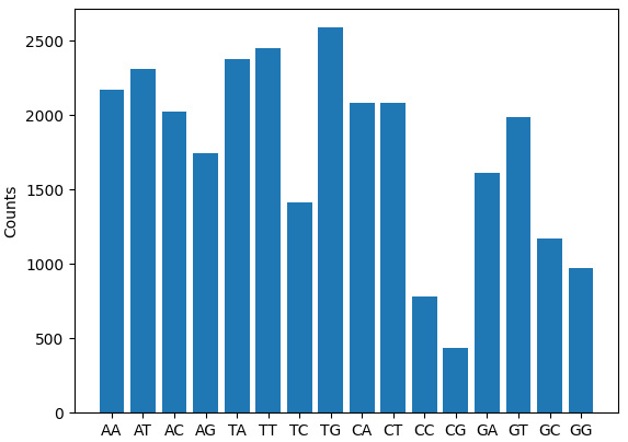
Figure 2.4 – Bar plot showing the dinucleotide count from the Covid-19 sequence

As you can see and expect, the expected dinucleotide counts vary, and now you can repeat the same on different viruses and compare all of them to understand their difference concerning dinucleotide content.

Modeling

So far, you have looked at some of the key steps of sequence analysis, such as data collection, data transformation, EDA, visualization, and so on. The next step would be modeling either using ML-based or statistical-based methods. Since we have the next chapter dedicated to ML-based modeling, we will not go into details of how that is done here but to wrap this real-world use case, we will save all the features that we have extracted so far into a file and get it ready for modeling.

Let’s create a Python script and combine all the code that we have written so far, which we can use for generating the features, and use that for modeling in subsequent chapters:

1. First, include the code related to the different features such as dinucleotide content, A, G, C, and T percentage, GC content, and length of the sequence:

   # covid19_features.py

   from Bio import SeqIO

   from Bio.SeqUtils import GC

   import pandas as pd

   nucl = ['A', 'T', 'C', 'G']

   final_dict = {}

   with open('covid19.fasta') as fh_in:

       with open("test.csv", 'w') as fh_out:

           for record in SeqIO.parse(fh_in, "fasta"):

               for n1 in nucl:

                   for n2 in nucl:

                       di = str(n1) + str(n2)

                       final_dict[di] = record.seq.count(di)

               A_count = record.seq.count('A')

               final_dict['A_count'] = round(A_count/len(record) * 100, 2)

               C_count = record.seq.count('C')

               final_dict['C_count'] = round(C_count/len(record) * 100, 2)

               G_count = record.seq.count('G')

               final_dict['G_count'] = round(G_count/len(record) * 100, 2)

               T_count = record.seq.count('T')

               final_dict['T_count'] = round(T_count/len(record) * 100, 2)

               final_dict['GC_content'] = round(GC(record.seq), 2)

               final_dict['Size'] = len(record)

All of this should be familiar from the preceding code.

2. Once you have the code for extracting the features, then you are ready to save them to a file using the following code:

   final_df = pd.DataFrame.from_dict([final_dict])

   final_df['virus'] = "Covid19"

   final_df.to_csv("covid19_features.csv", index=None)

3. Executing the script at the command prompt generates covid19_features.csv:

   $ python3.7 covid19_features.py

Before we end this section, let’s print the contents of the output file (covid19_features.csv):

$ cat covid19_features.csv

AA,AT,AC,AG,TA,TT,TC,TG,CA,CT,CC,CG,GA,GT,GC,GG,A_count,C_count,G_count,T_count,GC_content,Size,virus

2169,2308,2023,1742,2377,2454,1413,2589,2084,2081,784,439,1612,1990,1168,973,29.94,18.37,19.61,32.08,37.97,29903,Covid19

As you can see, we have combined all the features (A, G, T, and C content, GC content, and dinucleotide content) in a file and added a separate virus column to indicate where the features are coming from. Now, you can do the same with a few other viruses and then build a model, evaluate it, and then use that model to predict the type of virus from an unknown sequence. Isn’t this powerful?

Motif finder

A motif is a pattern in a nucleotide or amino acid sequence that has a specific structure. Sequence motifs play a key role in gene expression regulating both transcriptional and post-transcriptional levels. Motif mining is the foundation of gene function research. Currently, there have been innumerable algorithms including ML- and DL-based motif miners. The goal here is to utilize Biopython’s motifs module to access the functionalities of sequence motifs. Let’s understand how it is done now:

1. The motif method can be imported from the Biopython library shown as follows:

   >>> from Bio import motifs >>> from Bio.Seq import Seq

2. Let’s now create a simple DNA motif object as shown in the following code:

   >>> my_motif = [Seq("ACGT"), Seq("TCGA"), Seq("CGGC")]

Here, we are creating a list of Seq objects each containing a four-nucleotide sequence, and passing it to a my_motif variable.

3. Now, we will create a motif object from the seq object list and print the list:

   >>> seq = motifs.create(my_motif)

   >>> print(seq)

   ACGT

   TCGA

   CGGC

As expected, the motif object printed the three different seq objects.

4. One of the important attributes that are available for motif objects is counts, which prints the counts of each nucleotide at each position. This can also refer as the position frequency matrix (PFM). Printing this matrix is shown as follows:

   >>> print(seq.counts)

           0      1      2      3

   A:   1.00   0.00   0.00   1.00

   C:   1.00   2.00   0.00   1.00

   G:   0.00   1.00   3.00   0.00

   T:   1.00   0.00   0.00   1.00

What we see here is a matrix of nucleotide types and their position in the sequence along rows and columns, respectively, and counts in each of the cells.

5. You can also create a logo from the motif by running the following command:

   >>> seq.weblogo('my_motif.png')

This will generate a 'my_motif.png' file in the current working directory. Please note that you need to have internet access for this to work.

Figure 2.5 – Example logo generated from sequence motif

As you can see, Biopython is powerful in generating this kind of result without you needing to manually write functions to do it. Biopython would be extremely useful in the data processing stage of genomic data analysis, where the goal is to transform the raw data into processed data.

Summary

In this chapter, you were introduced to genomic data analysis for DNA sequencing data. First, we looked at the foundations of genomics and a brief history of DNA sequencing. Next, we explored in depth the genomic data analysis, the different types of data analysis, and a brief introduction to cloud computing for genomics data analysis. Then, we had a quick tutorial on using Biopython for analyzing genomic data. Finally, we applied the Biopython fundamentals to a real-world use case to understand how to perform sequence analysis.

Throughout this book, Python and Biopython are the main languages we will use to analyze genomic data. Biopython is a very powerful Python package for performing genomic data analysis with existing functions and methods that can be used out of the box. Many genomic and Data scientists routinely use Biopython for performing day-to-day jobs writing scripts for parsing the data or creating features for building ML and DL models.

Now that you have gained some understanding of genomic data analysis, let’s go ahead and investigate ML for genomics applications in the next chapter.