This chapter covers

• Representing real-world data as PyTorch tensors
• Working with a range of data types
• Loading data from a file
• Converting data to tensors
• Shaping tensors so they can be used as inputs for neural network models

In the previous chapter, we learned that tensors are the building blocks for data in PyTorch. Neural networks take tensors as input and produce tensors as outputs. In fact, all operations within a neural network and during optimization are operations between tensors, and all parameters (for example, weights and biases) in a neural network are tensors. Having a good sense of how to perform operations on tensors and index them effectively is central to using tools like PyTorch successfully. Now that you know the basics of tensors, your dexterity with them will grow as you make your way through the book.

Here’s a question that we can already address: how do we take a piece of data, a video, or a line of text, and represent it with a tensor in a way that is appropriate for training a deep learning model? This is what we’ll learn in this chapter. We’ll cover different types of data with a focus on the types relevant to this book and show how to represent that data as tensors. Then we’ll learn how to load the data from the most common on-disk formats and get a feel for those data types’ structure so we can see how to prepare them for training a neural network. Often, our raw data won’t be perfectly formed for the problem we’d like to solve, so we’ll have a chance to practice our tensor-manipulation skills with a few more interesting tensor operations.

Each section in this chapter will describe a data type, and each will come with its own dataset. While we’ve structured the chapter so that each data type builds on the previous one, feel free to skip around a bit if you’re so inclined.

We’ll be using a lot of image and volumetric data through the rest of the book, since those are common data types and they reproduce well in book format. We’ll also cover tabular data, time series, and text, as those will also be of interest to a number of our readers. Since a picture is worth a thousand words, we’ll start with image data. We’ll then demonstrate working with a three-dimensional array using medical data that represents patient anatomy as a volume. Next, we’ll work with tabular data about wines, just like what we’d find in a spreadsheet. After that, we’ll move to ordered tabular data, with a time-series dataset from a bike-sharing program. Finally, we’ll dip our toes into text data from Jane Austen. Text data retains its ordered aspect but introduces the problem of representing words as arrays of numbers.

In every section, we will stop where a deep learning researcher would start: right before feeding the data to a model. We encourage you to keep these datasets; they will constitute excellent material for when we start learning how to train neural network models in the next chapter.

4.1 Working with images

The introduction of convolutional neural networks revolutionized computer vision (see http://mng.bz/zjMa), and image-based systems have since acquired a whole new set of capabilities. Problems that required complex pipelines of highly tuned algorithmic building blocks are now solvable at unprecedented levels of performance by training end-to-end networks using paired input-and-desired-output examples. In order to participate in this revolution, we need to be able to load an image from common image formats and then transform the data into a tensor representation that has the various parts of the image arranged in the way PyTorch expects.

An image is represented as a collection of scalars arranged in a regular grid with a height and a width (in pixels). We might have a single scalar per grid point (the pixel), which would be represented as a grayscale image; or multiple scalars per grid point, which would typically represent different colors, as we saw in the previous chapter, or different features like depth from a depth camera.

Scalars representing values at individual pixels are often encoded using 8-bit integers, as in consumer cameras. In medical, scientific, and industrial applications, it is not unusual to find higher numerical precision, such as 12-bit or 16-bit. This allows a wider range or increased sensitivity in cases where the pixel encodes information about a physical property, like bone density, temperature, or depth.

4.1.1 Adding color channels

We mentioned colors earlier. There are several ways to encode colors into numbers.¹ The most common is RGB, where a color is defined by three numbers representing the intensity of red, green, and blue. We can think of a color channel as a grayscale intensity map of only the color in question, similar to what you’d see if you looked at the scene in question using a pair of pure red sunglasses. Figure 4.1 shows a rainbow, where each of the RGB channels captures a certain portion of the spectrum (the figure is simplified, in that it elides things like the orange and yellow bands being represented as a combination of red and green).

Figure 4.1 A rainbow, broken into red, green, and blue channels

The red band of the rainbow is brightest in the red channel of the image, while the blue channel has both the blue band of the rainbow and the sky as high-intensity. Note also that the white clouds are high-intensity in all three channels.

4.1.2 Loading an image file

Images come in several different file formats, but luckily there are plenty of ways to load images in Python. Let’s start by loading a PNG image using the imageio module (code/p1ch4/1_image_dog.ipynb).

Listing 4.1 code/p1ch4/1_image_dog.ipynb

# In[2]:
import imageio
 
img_arr = imageio.imread('../data/p1ch4/image-dog/bobby.jpg')
img_arr.shape
 
# Out[2]:
(720, 1280, 3)

Note We’ll use imageio throughout the chapter because it handles different data types with a uniform API. For many purposes, using TorchVision is a great default choice to deal with image and video data. We go with imageio here for somewhat lighter exploration.

At this point, img is a NumPy array-like object with three dimensions: two spatial dimensions, width and height; and a third dimension corresponding to the red, green, and blue channels. Any library that outputs a NumPy array will suffice to obtain a PyTorch tensor. The only thing to watch out for is the layout of the dimensions. PyTorch modules dealing with image data require tensors to be laid out as C × H × W : channels, height, and width, respectively.

4.1.3 Changing the layout

We can use the tensor’s permute method with the old dimensions for each new dimension to get to an appropriate layout. Given an input tensor H × W × C as obtained previously, we get a proper layout by having channel 2 first and then channels 0 and 1:

# In[3]:
img = torch.from_numpy(img_arr)
out = img.permute(2, 0, 1)

We’ve seen this previously, but note that this operation does not make a copy of the tensor data. Instead, out uses the same underlying storage as img and only plays with the size and stride information at the tensor level. This is convenient because the operation is very cheap; but just as a heads-up: changing a pixel in img will lead to a change in out.

Note also that other deep learning frameworks use different layouts. For instance, originally TensorFlow kept the channel dimension last, resulting in an H × W × C layout (it now supports multiple layouts). This strategy has pros and cons from a low-level performance standpoint, but for our concerns, it doesn’t make a difference as long as we reshape our tensors properly.

So far, we have described a single image. Following the same strategy we’ve used for earlier data types, to create a dataset of multiple images to use as an input for our neural networks, we store the images in a batch along the first dimension to obtain an N × C × H × W tensor.

As a slightly more efficient alternative to using stack to build up the tensor, we can preallocate a tensor of appropriate size and fill it with images loaded from a directory, like so:

# In[4]:
batch_size = 3
batch = torch.zeros(batch_size, 3, 256, 256, dtype=torch.uint8)

This indicates that our batch will consist of three RGB images 256 pixels in height and 256 pixels in width. Notice the type of the tensor: we’re expecting each color to be represented as an 8-bit integer, as in most photographic formats from standard consumer cameras. We can now load all PNG images from an input directory and store them in the tensor:

# In[5]:
import os
 
data_dir = '../data/p1ch4/image-cats/'
filenames = [name for name in os.listdir(data_dir)
             if os.path.splitext(name)[-1] == '.png']
for i, filename in enumerate(filenames):
    img_arr = imageio.imread(os.path.join(data_dir, filename))
    img_t = torch.from_numpy(img_arr)
    img_t = img_t.permute(2, 0, 1)
    img_t = img_t[:3]                   ❶
    batch[i] = img_t

❶ Here we keep only the first three channels. Sometimes images also have an alpha channel indicating transparency, but our network only wants RGB input.

4.1.4 Normalizing the data

We mentioned earlier that neural networks usually work with floating-point tensors as their input. Neural networks exhibit the best training performance when the input data ranges roughly from 0 to 1, or from -1 to 1 (this is an effect of how their building blocks are defined).

So a typical thing we’ll want to do is cast a tensor to floating-point and normalize the values of the pixels. Casting to floating-point is easy, but normalization is trickier, as it depends on what range of the input we decide should lie between 0 and 1 (or -1 and 1). One possibility is to just divide the values of the pixels by 255 (the maximum representable number in 8-bit unsigned):

# In[6]:
batch = batch.float()
batch /= 255.0

Another possibility is to compute the mean and standard deviation of the input data and scale it so that the output has zero mean and unit standard deviation across each channel:

# In[7]:
n_channels = batch.shape[1]
for c in range(n_channels):
    mean = torch.mean(batch[:, c])
    std = torch.std(batch[:, c])
    batch[:, c] = (batch[:, c] - mean) / std

Note Here, we normalize just a single batch of images because we do not know yet how to operate on an entire dataset. In working with images, it is good practice to compute the mean and standard deviation on all the training data in advance and then subtract and divide by these fixed, precomputed quantities. We saw this in the preprocessing for the image classifier in section 2.1.4.

We can perform several other operations on inputs, such as geometric transformations like rotations, scaling, and cropping. These may help with training or may be required to make an arbitrary input conform to the input requirements of a network, like the size of the image. We will stumble on quite a few of these strategies in section 12.6. For now, just remember that you have image-manipulation options available.

4.2 3D images: Volumetric data

We’ve learned how to load and represent 2D images, like the ones we take with a camera. In some contexts, such as medical imaging applications involving, say, CT (computed tomography) scans, we typically deal with sequences of images stacked along the head-to-foot axis, each corresponding to a slice across the human body. In CT scans, the intensity represents the density of the different parts of the body--lungs, fat, water, muscle, and bone, in order of increasing density--mapped from dark to bright when the CT scan is displayed on a clinical workstation. The density at each point is computed from the amount of X-rays reaching a detector after crossing through the body, with some complex math to deconvolve the raw sensor data into the full volume.

CTs have only a single intensity channel, similar to a grayscale image. This means that often, the channel dimension is left out in native data formats; so, similar to the last section, the raw data typically has three dimensions. By stacking individual 2D slices into a 3D tensor, we can build volumetric data representing the 3D anatomy of a subject. Unlike what we saw in figure 4.1, the extra dimension in figure 4.2 represents an offset in physical space, rather than a particular band of the visible spectrum.

Figure 4.2 Slices of a CT scan, from the top of the head to the jawline

Part 2 of this book will be devoted to tackling a medical imaging problem in the real world, so we won’t go into the details of medical-imaging data formats. For now, it suffices to say that there’s no fundamental difference between a tensor storing volumetric data versus image data. We just have an extra dimension, depth, after the channel dimension, leading to a 5D tensor of shape N × C × D × H × W.

4.2.1 Loading a specialized format

Let’s load a sample CT scan using the volread function in the imageio module, which takes a directory as an argument and assembles all Digital Imaging and Communications in Medicine (DICOM) files² in a series in a NumPy 3D array (code/p1ch4/ 2_volumetric_ct.ipynb).

Listing 4.2 code/p1ch4/2_volumetric_ct.ipynb

# In[2]:
import imageio
 
dir_path = "../data/p1ch4/volumetric-dicom/2-LUNG 3.0  B70f-04083"
vol_arr = imageio.volread(dir_path, 'DICOM')
vol_arr.shape
 
# Out[2]:
Reading DICOM (examining files): 1/99 files (1.0%99/99 files (100.0%)
  Found 1 correct series.
Reading DICOM (loading data): 31/99  (31.392/99  (92.999/99  (100.0%)
 
(99, 512, 512)

As was true in section 4.1.3, the layout is different from what PyTorch expects, due to having no channel information. So we’ll have to make room for the channel dimension using unsqueeze:

# In[3]:
vol = torch.from_numpy(vol_arr).float()
vol = torch.unsqueeze(vol, 0)
 
vol.shape
 
# Out[3]:
torch.Size([1, 99, 512, 512])

At this point we could assemble a 5D dataset by stacking multiple volumes along the batch direction, just as we did in the previous section. We’ll see a lot more CT data in part 2.

4.3 Representing tabular data

The simplest form of data we’ll encounter on a machine learning job is sitting in a spreadsheet, CSV file, or database. Whatever the medium, it’s a table containing one row per sample (or record), where columns contain one piece of information about our sample.

At first we are going to assume there’s no meaning to the order in which samples appear in the table: such a table is a collection of independent samples, unlike a time series, for instance, in which samples are related by a time dimension.

Columns may contain numerical values, like temperatures at specific locations; or labels, like a string expressing an attribute of the sample, like “blue.” Therefore, tabular data is typically not homogeneous: different columns don’t have the same type. We might have a column showing the weight of apples and another encoding their color in a label.

PyTorch tensors, on the other hand, are homogeneous. Information in PyTorch is typically encoded as a number, typically floating-point (though integer types and Boolean are supported as well). This numeric encoding is deliberate, since neural networks are mathematical entities that take real numbers as inputs and produce real numbers as output through successive application of matrix multiplications and nonlinear functions.

4.3.1 Using a real-world dataset

Our first job as deep learning practitioners is to encode heterogeneous, real-world data into a tensor of floating-point numbers, ready for consumption by a neural network. A large number of tabular datasets are freely available on the internet; see, for instance, https://github.com/caesar0301/awesome-public-datasets. Let’s start with something fun: wine! The Wine Quality dataset is a freely available table containing chemical characterizations of samples of vinho verde, a wine from north Portugal, together with a sensory quality score. The dataset for white wines can be downloaded here: http://mng.bz/90Ol. For convenience, we also created a copy of the dataset on the Deep Learning with PyTorch Git repository, under data/p1ch4/tabular-wine.

The file contains a comma-separated collection of values organized in 12 columns preceded by a header line containing the column names. The first 11 columns contain values of chemical variables, and the last column contains the sensory quality score from 0 (very bad) to 10 (excellent). These are the column names in the order they appear in the dataset:

fixed acidity
volatile acidity
citric acid
residual sugar
chlorides
free sulfur dioxide
total sulfur dioxide
density
pH
sulphates
alcohol
quality

A possible machine learning task on this dataset is predicting the quality score from chemical characterization alone. Don’t worry, though; machine learning is not going to kill wine tasting anytime soon. We have to get the training data from somewhere! As we can see in figure 4.3, we’re hoping to find a relationship between one of the chemical columns in our data and the quality column. Here, we’re expecting to see quality increase as sulfur decreases.

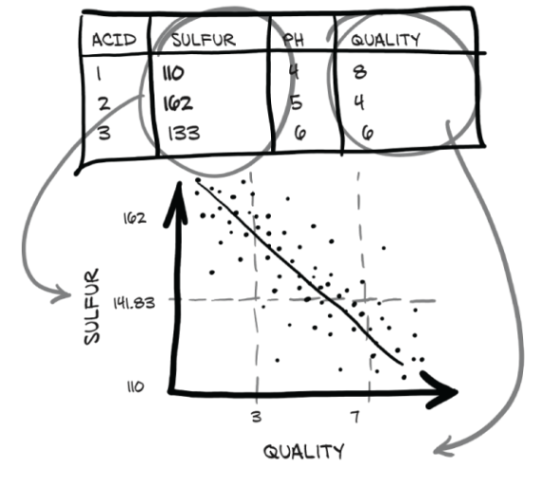
Figure 4.3 The (we hope) relationship between sulfur and quality in wine

4.3.2 Loading a wine data tensor

Before we can get to that, however, we need to be able to examine the data in a more usable way than opening the file in a text editor. Let’s see how we can load the data using Python and then turn it into a PyTorch tensor. Python offers several options for quickly loading a CSV file. Three popular options are

• The csv module that ships with Python

• NumPy

• Pandas

The third option is the most time- and memory-efficient. However, we’ll avoid introducing an additional library in our learning trajectory just because we need to load a file. Since we already introduced NumPy in the previous section, and PyTorch has excellent NumPy interoperability, we’ll go with that. Let’s load our file and turn the resulting NumPy array into a PyTorch tensor (code/p1ch4/3_tabular_wine.ipynb).

Listing 4.3 code/p1ch4/3_tabular_wine.ipynb

# In[2]:
import csv
wine_path = "../data/p1ch4/tabular-wine/winequality-white.csv"
wineq_numpy = np.loadtxt(wine_path, dtype=np.float32, delimiter=";",
                         skiprows=1)
wineq_numpy
 
# Out[2]:
array([[ 7.  ,  0.27,  0.36, ...,  0.45,  8.8 ,  6.  ],
       [ 6.3 ,  0.3 ,  0.34, ...,  0.49,  9.5 ,  6.  ],
       [ 8.1 ,  0.28,  0.4 , ...,  0.44, 10.1 ,  6.  ],
       ...,
       [ 6.5 ,  0.24,  0.19, ...,  0.46,  9.4 ,  6.  ],
       [ 5.5 ,  0.29,  0.3 , ...,  0.38, 12.8 ,  7.  ],
       [ 6.  ,  0.21,  0.38, ...,  0.32, 11.8 ,  6.  ]], dtype=float32)

Here we just prescribe what the type of the 2D array should be (32-bit floating-point), the delimiter used to separate values in each row, and the fact that the first line should not be read since it contains the column names. Let’s check that all the data has been read

# In[3]:
col_list = next(csv.reader(open(wine_path), delimiter=';'))
 
wineq_numpy.shape, col_list
 
# Out[3]:
((4898, 12),
 ['fixed acidity',
  'volatile acidity',
  'citric acid',
  'residual sugar',
  'chlorides',
  'free sulfur dioxide',
  'total sulfur dioxide',
  'density',
  'pH',
  'sulphates',
  'alcohol',
  'quality'])

and proceed to convert the NumPy array to a PyTorch tensor:

# In[4]:
wineq = torch.from_numpy(wineq_numpy)
 
wineq.shape, wineq.dtype
 
# Out[4]:
(torch.Size([4898, 12]), torch.float32)

At this point, we have a floating-point torch.Tensor containing all the columns, including the last, which refers to the quality score. ³

4.3.3 Representing scores

We could treat the score as a continuous variable, keep it as a real number, and perform a regression task, or treat it as a label and try to guess the label from the chemical analysis in a classification task. In both approaches, we will typically remove the score from the tensor of input data and keep it in a separate tensor, so that we can use the score as the ground truth without it being input to our model:

# In[5]:
data = wineq[:, :-1]     ❶
data, data.shape
 
# Out[5]:
(tensor([[ 7.00,  0.27,  ...,  0.45,  8.80],
         [ 6.30,  0.30,  ...,  0.49,  9.50],
         ...,
         [ 5.50,  0.29,  ...,  0.38, 12.80],
         [ 6.00,  0.21,  ...,  0.32, 11.80]]), torch.Size([4898, 11]))

# In[6]:
target = wineq[:, -1]    ❷
target, target.shape

# Out[6]:
(tensor([6., 6.,  ..., 7., 6.]), torch.Size([4898]))

❶ Selects all rows and all columns except the last

❷ Selects all rows and the last column

If we want to transform the target tensor in a tensor of labels, we have two options, depending on the strategy or what we use the categorical data for. One is simply to treat labels as an integer vector of scores:

# In[7]:
target = wineq[:, -1].long()
target

# Out[7]:
tensor([6, 6,  ..., 7, 6])

If targets were string labels, like wine color, assigning an integer number to each string would let us follow the same approach.

4.3.4 One-hot encoding

The other approach is to build a one-hot encoding of the scores: that is, encode each of the 10 scores in a vector of 10 elements, with all elements set to 0 but one, at a different index for each score. This way, a score of 1 could be mapped onto the vector (1,0,0,0,0,0,0,0,0,0), a score of 5 onto (0,0,0,0,1,0,0,0,0,0), and so on. Note that the fact that the score corresponds to the index of the nonzero element is purely incidental: we could shuffle the assignment, and nothing would change from a classification standpoint.

There’s a marked difference between the two approaches. Keeping wine quality scores in an integer vector of scores induces an ordering on the scores--which might be totally appropriate in this case, since a score of 1 is lower than a score of 4. It also induces some sort of distance between scores: that is, the distance between 1 and 3 is the same as the distance between 2 and 4. If this holds for our quantity, then great. If, on the other hand, scores are purely discrete, like grape variety, one-hot encoding will be a much better fit, as there’s no implied ordering or distance. One-hot encoding is also appropriate for quantitative scores when fractional values in between integer scores, like 2.4, make no sense for the application--for when the score is either this or that.

We can achieve one-hot encoding using the scatter_ method, which fills the tensor with values from a source tensor along the indices provided as arguments:

# In[8]:
target_onehot = torch.zeros(target.shape[0], 10)
 
target_onehot.scatter_(1, target.unsqueeze(1), 1.0)
 
# Out[8]:
tensor([[0., 0.,  ..., 0., 0.],
        [0., 0.,  ..., 0., 0.],
        ...,
        [0., 0.,  ..., 0., 0.],
        [0., 0.,  ..., 0., 0.]])

Let’s see what scatter_ does. First, we notice that its name ends with an underscore. As you learned in the previous chapter, this is a convention in PyTorch that indicates the method will not return a new tensor, but will instead modify the tensor in place. The arguments for scatter_ are as follows:

• The dimension along which the following two arguments are specified

• A column tensor indicating the indices of the elements to scatter

• A tensor containing the elements to scatter or a single scalar to scatter (1, in this case)

In other words, the previous invocation reads, “For each row, take the index of the target label (which coincides with the score in our case) and use it as the column index to set the value 1.0.” The end result is a tensor encoding categorical information.

The second argument of scatter_, the index tensor, is required to have the same number of dimensions as the tensor we scatter into. Since target_onehot has two dimensions (4,898 × 10), we need to add an extra dummy dimension to target using unsqueeze:

# In[9]:
target_unsqueezed = target.unsqueeze(1)
target_unsqueezed
 
# Out[9]:
tensor([[6],
        [6],
        ...,
        [7],
        [6]])

The call to unsqueeze adds a singleton dimension, from a 1D tensor of 4,898 elements to a 2D tensor of size (4,898 × 1), without changing its contents--no extra elements are added; we just decided to use an extra index to access the elements. That is, we access the first element of target as target[0] and the first element of its unsqueezed counterpart as target_unsqueezed[0,0].

PyTorch allows us to use class indices directly as targets while training neural networks. However, if we wanted to use the score as a categorical input to the network, we would have to transform it to a one-hot-encoded tensor.

4.3.5 When to categorize

Now we have seen ways to deal with both continuous and categorical data. You may wonder what the deal is with the ordinal case discussed in the earlier sidebar. There is no general recipe for it; most commonly, such data is either treated as categorical (losing the ordering part, and hoping that maybe our model will pick it up during training if we only have a few categories) or continuous (introducing an arbitrary notion of distance). We will do the latter for the weather situation in figure 4.5. We summarize our data mapping in a small flow chart in figure 4.4.

Figure 4.4 How to treat columns with continuous, ordinal, and categorical data

Let’s go back to our data tensor, containing the 11 variables associated with the chemical analysis. We can use the functions in the PyTorch Tensor API to manipulate our data in tensor form. Let’s first obtain the mean and standard deviations for each column:

# In[10]:
data_mean = torch.mean(data, dim=0)
data_mean
 
# Out[10]:
tensor([6.85e+00, 2.78e-01, 3.34e-01, 6.39e+00, 4.58e-02, 3.53e+01,
        1.38e+02, 9.94e-01, 3.19e+00, 4.90e-01, 1.05e+01])

# In[11]:
data_var = torch.var(data, dim=0)
data_var
 
# Out[11]:
tensor([7.12e-01, 1.02e-02, 1.46e-02, 2.57e+01, 4.77e-04, 2.89e+02,
        1.81e+03, 8.95e-06, 2.28e-02, 1.30e-02, 1.51e+00])

In this case, dim=0 indicates that the reduction is performed along dimension 0. At this point, we can normalize the data by subtracting the mean and dividing by the standard deviation, which helps with the learning process (we’ll discuss this in more detail in chapter 5, in section 5.4.4):

# In[12]:
data_normalized = (data - data_mean) / torch.sqrt(data_var)
data_normalized
 
# Out[12]:
tensor([[ 1.72e-01, -8.18e-02,  ..., -3.49e-01, -1.39e+00],
        [-6.57e-01,  2.16e-01,  ...,  1.35e-03, -8.24e-01],
        ...,
        [-1.61e+00,  1.17e-01,  ..., -9.63e-01,  1.86e+00],
        [-1.01e+00, -6.77e-01,  ..., -1.49e+00,  1.04e+00]])

4.3.6 Finding thresholds

Next, let’s start to look at the data with an eye to seeing if there is an easy way to tell good and bad wines apart at a glance. First, we’re going to determine which rows in target correspond to a score less than or equal to 3:

# In[13]:
bad_indexes = target <= 3                                ❶
bad_indexes.shape, bad_indexes.dtype, bad_indexes.sum()
 
# Out[13]:
(torch.Size([4898]), torch.bool, tensor(20))

❶ PyTorch also provides comparison functions, here torch.le(target, 3), but using operators seems to be a good standard.

Note that only 20 of the bad_indexes entries are set to True! By using a feature in PyTorch called advanced indexing, we can use a tensor with data type torch.bool to index the data tensor. This will essentially filter data to be only items (or rows) corresponding to True in the indexing tensor. The bad_indexes tensor has the same shape as target, with values of False or True depending on the outcome of the comparison between our threshold and each element in the original target tensor:

# In[14]:
bad_data = data[bad_indexes]
bad_data.shape
 
# Out[14]:
torch.Size([20, 11])

Note that the new bad_data tensor has 20 rows, the same as the number of rows with True in the bad_indexes tensor. It retains all 11 columns. Now we can start to get information about wines grouped into good, middling, and bad categories. Let’s take the .mean() of each column:

# In[15]:
bad_data = data[target <= 3]
mid_data = data[(target > 3) & (target < 7)]    ❶
good_data = data[target >= 7]
 
bad_mean = torch.mean(bad_data, dim=0)
mid_mean = torch.mean(mid_data, dim=0)
good_mean = torch.mean(good_data, dim=0)
 
for i, args in enumerate(zip(col_list, bad_mean, mid_mean, good_mean)):
    print('{:2} {:20} {:6.2f} {:6.2f} {:6.2f}'.format(i, *args))
 
# Out[15]:
 0 fixed acidity          7.60   6.89   6.73
 1 volatile acidity       0.33   0.28   0.27
 2 citric acid            0.34   0.34   0.33
 3 residual sugar         6.39   6.71   5.26
 4 chlorides              0.05   0.05   0.04
 5 free sulfur dioxide   53.33  35.42  34.55
 6 total sulfur dioxide 170.60 141.83 125.25
 7 density                0.99   0.99   0.99
 8 pH                     3.19   3.18   3.22
 9 sulphates              0.47   0.49   0.50
10 alcohol               10.34  10.26  11.42

❶ For Boolean NumPy arrays and PyTorch tensors, the & operator does a logical “and” operation.

It looks like we’re on to something here: at first glance, the bad wines seem to have higher total sulfur dioxide, among other differences. We could use a threshold on total sulfur dioxide as a crude criterion for discriminating good wines from bad ones. Let’s get the indexes where the total sulfur dioxide column is below the midpoint we calculated earlier, like so:

# In[16]:
total_sulfur_threshold = 141.83
total_sulfur_data = data[:,6]
predicted_indexes = torch.lt(total_sulfur_data, total_sulfur_threshold)
 
predicted_indexes.shape, predicted_indexes.dtype, predicted_indexes.sum()
 
# Out[16]:
(torch.Size([4898]), torch.bool, tensor(2727))

This means our threshold implies that just over half of all the wines are going to be high quality. Next, we’ll need to get the indexes of the actually good wines:

# In[17]:
actual_indexes = target > 5
 
actual_indexes.shape, actual_indexes.dtype, actual_indexes.sum()
 
# Out[17]:
(torch.Size([4898]), torch.bool, tensor(3258))

Since there are about 500 more actually good wines than our threshold predicted, we already have hard evidence that it’s not perfect. Now we need to see how well our predictions line up with the actual rankings. We will perform a logical “and” between our prediction indexes and the actual good indexes (remember that each is just an array of zeros and ones) and use that intersection of wines-in-agreement to determine how well we did:

# In[18]:
n_matches = torch.sum(actual_indexes & predicted_indexes).item()
n_predicted = torch.sum(predicted_indexes).item()
n_actual = torch.sum(actual_indexes).item()
 
n_matches, n_matches / n_predicted, n_matches / n_actual
 
# Out[18]:
(2018, 0.74000733406674, 0.6193984039287906)

We got around 2,000 wines right! Since we predicted 2,700 wines, this gives us a 74% chance that if we predict a wine to be high quality, it actually is. Unfortunately, there are 3,200 good wines, and we only identified 61% of them. Well, we got what we signed up for; that’s barely better than random! Of course, this is all very naive: we know for sure that multiple variables contribute to wine quality, and the relationships between the values of these variables and the outcome (which could be the actual score, rather than a binarized version of it) is likely more complicated than a simple threshold on a single value.

Indeed, a simple neural network would overcome all of these limitations, as would a lot of other basic machine learning methods. We’ll have the tools to tackle this problem after the next two chapters, once we have learned how to build our first neural network from scratch. We will also revisit how to better grade our results in chapter 12. Let’s move on to other data types for now.

4.4 Working with time series

In the previous section, we covered how to represent data organized in a flat table. As we noted, every row in the table was independent from the others; their order did not matter. Or, equivalently, there was no column that encoded information about what rows came earlier and what came later.

Going back to the wine dataset, we could have had a “year” column that allowed us to look at how wine quality evolved year after year. Unfortunately, we don’t have such data at hand, but we’re working hard on manually collecting the data samples, bottle by bottle. (Stuff for our second edition.) In the meantime, we’ll switch to another interesting dataset: data from a Washington, D.C., bike-sharing system reporting the hourly count of rental bikes in 2011-2012 in the Capital Bikeshare system, along with weather and seasonal information (available here: http://mng.bz/jgOx). Our goal will be to take a flat, 2D dataset and transform it into a 3D one, as shown in figure 4.5.

Figure 4.5 Transforming a 1D, multichannel dataset into a 2D, multichannel dataset by separating the date and hour of each sample into separate axes

4.4.1 Adding a time dimension

In the source data, each row is a separate hour of data (figure 4.5 shows a transposed version of this to better fit on the printed page). We want to change the row-per-hour organization so that we have one axis that increases at a rate of one day per index increment, and another axis that represents the hour of the day (independent of the date). The third axis will be our different columns of data (weather, temperature, and so on).

Let’s load the data (code/p1ch4/4_time_series_bikes.ipynb).

Listing 4.4 code/p1ch4/4_time_series_bikes.ipynb

# In[2]:
bikes_numpy = np.loadtxt(
    "../data/p1ch4/bike-sharing-dataset/hour-fixed.csv",
    dtype=np.float32,
    delimiter=",",
    skiprows=1,
    converters={1: lambda x: float(x[8:10])})     ❶
bikes = torch.from_numpy(bikes_numpy)
bikes
 
# Out[2]:
tensor([[1.0000e+00, 1.0000e+00,  ..., 1.3000e+01, 1.6000e+01],
        [2.0000e+00, 1.0000e+00,  ..., 3.2000e+01, 4.0000e+01],
        ...,
        [1.7378e+04, 3.1000e+01,  ..., 4.8000e+01, 6.1000e+01],
        [1.7379e+04, 3.1000e+01,  ..., 3.7000e+01, 4.9000e+01]])

❶ Converts date strings to numbers corresponding to the day of the month in column 1

For every hour, the dataset reports the following variables:

• Index of record: instant

• Day of month: day

• Season: season (1: spring, 2: summer, 3: fall, 4: winter)

• Year: yr (0: 2011, 1: 2012)

• Month: mnth (1 to 12)

• Hour: hr (0 to 23)

• Holiday status: holiday

• Day of the week: weekday

• Working day status: workingday

• Weather situation: weathersit (1: clear, 2:mist, 3: light rain/snow, 4: heavy rain/snow)

• Temperature in °C: temp

• Perceived temperature in °C: atemp

• Humidity: hum

• Wind speed: windspeed

• Number of casual users: casual

• Number of registered users: registered

• Count of rental bikes: cnt

In a time series dataset such as this one, rows represent successive time-points: there is a dimension along which they are ordered. Sure, we could treat each row as independent and try to predict the number of circulating bikes based on, say, a particular time of day regardless of what happened earlier. However, the existence of an ordering gives us the opportunity to exploit causal relationships across time. For instance, it allows us to predict bike rides at one time based on the fact that it was raining at an earlier time. For the time being, we’re going to focus on learning how to turn our bike-sharing dataset into something that our neural network will be able to ingest in fixed-size chunks.

This neural network model will need to see a number of sequences of values for each different quantity, such as ride count, time of day, temperature, and weather conditions: N parallel sequences of size C. C stands for channel, in neural network parlance, and is the same as column for 1D data like we have here. The N dimension represents the time axis, here one entry per hour.

4.4.2 Shaping the data by time period

We might want to break up the two-year dataset into wider observation periods, like days. This way we’ll have N (for number of samples) collections of C sequences of length L. In other words, our time series dataset would be a tensor of dimension 3 and shape N × C × L. The C would remain our 17 channels, while L would be 24: 1 per hour of the day. There’s no particular reason why we must use chunks of 24 hours, though the general daily rhythm is likely to give us patterns we can exploit for predictions. We could also use 7 × 24 = 168 hour blocks to chunk by week instead, if we desired. All of this depends, naturally, on our dataset having the right size--the number of rows must be a multiple of 24 or 168. Also, for this to make sense, we cannot have gaps in the time series.

Let’s go back to our bike-sharing dataset. The first column is the index (the global ordering of the data), the second is the date, and the sixth is the time of day. We have everything we need to create a dataset of daily sequences of ride counts and other exogenous variables. Our dataset is already sorted, but if it were not, we could use torch.sort on it to order it appropriately.

Note The version of the file we’re using, hour-fixed.csv, has had some processing done to include rows missing from the original dataset. We presume that the missing hours had zero bike active (they were typically in the early morning hours).

All we have to do to obtain our daily hours dataset is view the same tensor in batches of 24 hours. Let’s take a look at the shape and strides of our bikes tensor:

# In[3]:
bikes.shape, bikes.stride()
 
# Out[3]:
(torch.Size([17520, 17]), (17, 1))

That’s 17,520 hours, 17 columns. Now let’s reshape the data to have 3 axes--day, hour, and then our 17 columns:

# In[4]:
daily_bikes = bikes.view(-1, 24, bikes.shape[1])
daily_bikes.shape, daily_bikes.stride()
 
# Out[4]:
(torch.Size([730, 24, 17]), (408, 17, 1))

What happened here? First, bikes.shape[1] is 17, the number of columns in the bikes tensor. But the real crux of this code is the call to view, which is really important: it changes the way the tensor looks at the same data as contained in storage.

As you learned in the previous chapter, calling view on a tensor returns a new tensor that changes the number of dimensions and the striding information, without changing the storage. This means we can rearrange our tensor at basically zero cost, because no data will be copied. Our call to view requires us to provide the new shape for the returned tensor. We use -1 as a placeholder for “however many indexes are left, given the other dimensions and the original number of elements.”

Remember also from the previous chapter that storage is a contiguous, linear container for numbers (floating-point, in this case). Our bikes tensor will have each row stored one after the other in its corresponding storage. This is confirmed by the output from the call to bikes.stride() earlier.

For daily_bikes, the stride is telling us that advancing by 1 along the hour dimension (the second dimension) requires us to advance by 17 places in the storage (or one set of columns); whereas advancing along the day dimension (the first dimension) requires us to advance by a number of elements equal to the length of a row in the storage times 24 (here, 408, which is 17 × 24).

We see that the rightmost dimension is the number of columns in the original dataset. Then, in the middle dimension, we have time, split into chunks of 24 sequential hours. In other words, we now have N sequences of L hours in a day, for C channels. To get to our desired N × C × L ordering, we need to transpose the tensor:

# In[5]:
daily_bikes = daily_bikes.transpose(1, 2)
daily_bikes.shape, daily_bikes.stride()
 
# Out[5]:
(torch.Size([730, 17, 24]), (408, 1, 17))

Now let’s apply some of the techniques we learned earlier to this dataset.

4.4.3 Ready for training

The “weather situation” variable is ordinal. It has four levels: 1 for good weather, and 4 for, er, really bad. We could treat this variable as categorical, with levels interpreted as labels, or as a continuous variable. If we decided to go with categorical, we would turn the variable into a one-hot-encoded vector and concatenate the columns with the dataset.⁴

In order to make it easier to render our data, we’re going to limit ourselves to the first day for a moment. We initialize a zero-filled matrix with a number of rows equal to the number of hours in the day and number of columns equal to the number of weather levels:

# In[6]:
first_day = bikes[:24].long()
weather_onehot = torch.zeros(first_day.shape[0], 4)
first_day[:,9]

# Out[6]:
tensor([1, 1, 1, 1, 1, 2, 1, 1, 1, 1, 1, 1, 1, 2, 2, 2, 2, 2, 3, 3, 2, 2,
        2, 2])

Then we scatter ones into our matrix according to the corresponding level at each row. Remember the use of unsqueeze to add a singleton dimension as we did in the previous sections:

# In[7]:
weather_onehot.scatter_(
    dim=1,
    index=first_day[:,9].unsqueeze(1).long() - 1,    ❶
    value=1.0)

# Out[7]:
tensor([[1., 0., 0., 0.],
        [1., 0., 0., 0.],
        ...,
        [0., 1., 0., 0.],
        [0., 1., 0., 0.]])

❶ Decreases the values by 1 because weather situation ranges from 1 to 4, while indices are 0-based

Our day started with weather “1” and ended with “2,” so that seems right.

Last, we concatenate our matrix to our original dataset using the cat function. Let’s look at the first of our results:

# In[8]:
torch.cat((bikes[:24], weather_onehot), 1)[:1]

# Out[8]:
tensor([[ 1.0000,  1.0000,  1.0000,  0.0000,  1.0000,  0.0000,  0.0000,
          6.0000,  0.0000,  1.0000,  0.2400,  0.2879,  0.8100,  0.0000,
          3.0000, 13.0000, 16.0000,  1.0000,  0.0000,  0.0000,  0.0000]])

Here we prescribed our original bikes dataset and our one-hot-encoded “weather situation” matrix to be concatenated along the column dimension (that is, 1). In other words, the columns of the two datasets are stacked together; or, equivalently, the new one-hot-encoded columns are appended to the original dataset. For cat to succeed, it is required that the tensors have the same size along the other dimensions--the row dimension, in this case. Note that our new last four columns are 1, 0, 0, 0, exactly as we would expect with a weather value of 1. We could have done the same with the reshaped daily_bikes tensor. Remember that it is shaped (B, C, L), where L = 24. We first create the zero tensor, with the same B and L, but with the number of additional columns as C :

# In[9]:
daily_weather_onehot = torch.zeros(daily_bikes.shape[0], 4,
                                   daily_bikes.shape[2])
daily_weather_onehot.shape
 
# Out[9]:
torch.Size([730, 4, 24])

Then we scatter the one-hot encoding into the tensor in the C dimension. Since this operation is performed in place, only the content of the tensor will change:

# In[10]:
daily_weather_onehot.scatter_(
    1, daily_bikes[:,9,:].long().unsqueeze(1) - 1, 1.0)
daily_weather_onehot.shape
 
# Out[10]:
torch.Size([730, 4, 24])

And we concatenate along the C dimension:

# In[11]:
daily_bikes = torch.cat((daily_bikes, daily_weather_onehot), dim=1)

We mentioned earlier that this is not the only way to treat our “weather situation” variable. Indeed, its labels have an ordinal relationship, so we could pretend they are special values of a continuous variable. We could just transform the variable so that it runs from 0.0 to 1.0:

# In[12]:
daily_bikes[:, 9, :] = (daily_bikes[:, 9, :] - 1.0) / 3.0

As we mentioned in the previous section, rescaling variables to the [0.0, 1.0] interval or the [-1.0, 1.0] interval is something we’ll want to do for all quantitative variables, like temperature (column 10 in our dataset). We’ll see why later; for now, let’s just say that this is beneficial to the training process.

There are multiple possibilities for rescaling variables. We can either map their range to [0.0, 1.0]

# In[13]:
temp = daily_bikes[:, 10, :]
temp_min = torch.min(temp)
temp_max = torch.max(temp)
daily_bikes[:, 10, :] = ((daily_bikes[:, 10, :] - temp_min)
                         / (temp_max - temp_min))

or subtract the mean and divide by the standard deviation:

# In[14]:
temp = daily_bikes[:, 10, :]
daily_bikes[:, 10, :] = ((daily_bikes[:, 10, :] - torch.mean(temp))
                         / torch.std(temp))

In the latter case, our variable will have 0 mean and unitary standard deviation. If our variable were drawn from a Gaussian distribution, 68% of the samples would sit in the [-1.0, 1.0] interval.

Great: we’ve built another nice dataset, and we’ve seen how to deal with time series data. For this tour d’horizon, it’s important only that we got an idea of how a time series is laid out and how we can wrangle the data in a form that a network will digest.

Other kinds of data look like a time series, in that there is a strict ordering. Top two on the list? Text and audio. We’ll take a look at text next, and the “Conclusion” section has links to additional examples for audio.

4.5 Representing text

Deep learning has taken the field of natural language processing (NLP) by storm, particularly using models that repeatedly consume a combination of new input and previous model output. These models are called recurrent neural networks (RNNs), and they have been applied with great success to text categorization, text generation, and automated translation systems. More recently, a class of networks called transformers with a more flexible way to incorporate past information has made a big splash. Previous NLP workloads were characterized by sophisticated multistage pipelines that included rules encoding the grammar of a language.⁵ Now, state-of-the-art work trains networks end to end on large corpora starting from scratch, letting those rules emerge from the data. For the last several years, the most-used automated translation systems available as services on the internet have been based on deep learning.

Our goal in this section is to turn text into something a neural network can process: a tensor of numbers, just like our previous cases. If we can do that and later choose the right architecture for our text-processing job, we’ll be in the position of doing NLP with PyTorch. We see right away how powerful this all is: we can achieve state-of-the-art performance on a number of tasks in different domains with the same PyTorch tools; we just need to cast our problem in the right form. The first part of this job is reshaping the data.

4.5.1 Converting text to numbers

There are two particularly intuitive levels at which networks operate on text: at the character level, by processing one character at a time, and at the word level, where individual words are the finest-grained entities to be seen by the network. The technique with which we encode text information into tensor form is the same whether we operate at the character level or the word level. And it’s not magic, either. We stumbled upon it earlier: one-hot encoding.

Let’s start with a character-level example. First, let’s get some text to process. An amazing resource here is Project Gutenberg (www.gutenberg.org), a volunteer effort to digitize and archive cultural work and make it available for free in open formats, including plain text files. If we’re aiming at larger-scale corpora, the Wikipedia corpus stands out: it’s the complete collection of Wikipedia articles, containing 1.9 billion words and more than 4.4 million articles. Several other corpora can be found at the English Corpora website (www.english-corpora.org).

Let’s load Jane Austen’s Pride and Prejudice from the Project Gutenberg website: www.gutenberg.org/files/1342/1342-0.txt. We’ll just save the file and read it in (code/p1ch4/5_text_jane_austen.ipynb).

Listing 4.5 code/p1ch4/5_text_jane_austen.ipynb

# In[2]:
with open('../data/p1ch4/jane-austen/1342-0.txt', encoding='utf8') as f:
    text = f.read()

4.5.2 One-hot-encoding characters

There’s one more detail we need to take care of before we proceed: encoding. This is a pretty vast subject, and we will just touch on it. Every written character is represented by a code: a sequence of bits of appropriate length so that each character can be uniquely identified. The simplest such encoding is ASCII (American Standard Code for Information Interchange), which dates back to the 1960s. ASCII encodes 128 characters using 128 integers. For instance, the letter a corresponds to binary 1100001 or decimal 97, the letter b to binary 1100010 or decimal 98, and so on. The encoding fits 8 bits, which was a big bonus in 1965.

Note 128 characters are clearly not enough to account for all the glyphs, accents, ligatures, and so on that are needed to properly represent written text in languages other than English. To this end, a number of encodings have been developed that use a larger number of bits as code for a wider range of characters. That wider range of characters was standardized as Unicode, which maps all known characters to numbers, with the representation in bits of those numbers provided by a specific encoding. Popular encodings are UTF-8, UTF-16, and UTF-32, in which the numbers are a sequence of 8-, 16-, or 32-bit integers, respectively. Strings in Python 3.x are Unicode strings.

We are going to one-hot encode our characters. It is instrumental to limit the one-hot encoding to a character set that is useful for the text being analyzed. In our case, since we loaded text in English, it is safe to use ASCII and deal with a small encoding. We could also make all of the characters lowercase, to reduce the number of different characters in our encoding. Similarly, we could screen out punctuation, numbers, or other characters that aren’t relevant to our expected kinds of text. This may or may not make a practical difference to a neural network, depending on the task at hand.

At this point, we need to parse through the characters in the text and provide a one-hot encoding for each of them. Each character will be represented by a vector of length equal to the number of different characters in the encoding. This vector will contain all zeros except a one at the index corresponding to the location of the character in the encoding.

We first split our text into a list of lines and pick an arbitrary line to focus on:

# In[3]:
lines = text.split('
')
line = lines[200]
line
 
# Out[3]:
'“Impossible, Mr. Bennet, impossible, when I am not acquainted with him'

Let’s create a tensor that can hold the total number of one-hot-encoded characters for the whole line:

# In[4]:
letter_t = torch.zeros(len(line), 128)    ❶
letter_t.shape
 
# Out[4]:
torch.Size([70, 128])

❶ 128 hardcoded due to the limits of ASCII

Note that letter_t holds a one-hot-encoded character per row. Now we just have to set a one on each row in the correct position so that each row represents the correct character. The index where the one has to be set corresponds to the index of the character in the encoding:

# In[5]:
for i, letter in enumerate(line.lower().strip()):
    letter_index = ord(letter) if ord(letter) < 128 else 0     ❶
    letter_t[i][letter_index] = 1

❶ The text uses directional double quotes, which are not valid ASCII, so we screen them out here.

4.5.3 One-hot encoding whole words

We have one-hot encoded our sentence into a representation that a neural network could digest. Word-level encoding can be done the same way by establishing a vocabulary and one-hot encoding sentences--sequences of words--along the rows of our tensor. Since a vocabulary has many words, this will produce very wide encoded vectors, which may not be practical. We will see in the next section that there is a more efficient way to represent text at the word level, using embeddings. For now, let’s stick with one-hot encodings and see what happens.

We’ll define clean_words, which takes text and returns it in lowercase and stripped of punctuation. When we call it on our “Impossible, Mr. Bennet” line, we get the following:

# In[6]:
def clean_words(input_str):
    punctuation = '.,;:"!?”“_-'
    word_list = input_str.lower().replace('
',' ').split()
    word_list = [word.strip(punctuation) for word in word_list]
    return word_list
 
words_in_line = clean_words(line)
line, words_in_line
 
# Out[6]:
('“Impossible, Mr. Bennet, impossible, when I am not acquainted with him',
 ['impossible',
  'mr',
  'bennet',
  'impossible',
  'when',
  'i',
  'am',
  'not',
  'acquainted',
  'with',
  'him'])

Next, let’s build a mapping of words to indexes in our encoding:

# In[7]:
word_list = sorted(set(clean_words(text)))
word2index_dict = {word: i for (i, word) in enumerate(word_list)}
 
len(word2index_dict), word2index_dict['impossible']
 
# Out[7]:
(7261, 3394)

Note that word2index_dict is now a dictionary with words as keys and an integer as a value. We will use it to efficiently find the index of a word as we one-hot encode it. Let’s now focus on our sentence: we break it up into words and one-hot encode it--that is, we populate a tensor with one one-hot-encoded vector per word. We create an empty vector and assign the one-hot-encoded values of the word in the sentence:

# In[8]:
word_t = torch.zeros(len(words_in_line), len(word2index_dict))
for i, word in enumerate(words_in_line):
    word_index = word2index_dict[word]
    word_t[i][word_index] = 1
    print('{:2} {:4} {}'.format(i, word_index, word))
 
print(word_t.shape)
 
 
# Out[8]:
 0 3394 impossible
 1 4305 mr
 2  813 bennet
 3 3394 impossible
 4 7078 when
 5 3315 i
 6  415 am
 7 4436 not
 8  239 acquainted
 9 7148 with
10 3215 him
torch.Size([11, 7261])

At this point, tensor represents one sentence of length 11 in an encoding space of size 7,261, the number of words in our dictionary. Figure 4.6 compares the gist of our two options for splitting text (and using the embeddings we’ll look at in the next section).

The choice between character-level and word-level encoding leaves us to make a trade-off. In many languages, there are significantly fewer characters than words: representing characters has us representing just a few classes, while representing words requires us to represent a very large number of classes and, in any practical application, deal with words that are not in the dictionary. On the other hand, words convey much more meaning than individual characters, so a representation of words is considerably more informative by itself. Given the stark contrast between these two options, it is perhaps unsurprising that intermediate ways have been sought, found, and applied with great success: for example, the byte pair encoding method⁶ starts with a dictionary of individual letters but then iteratively adds the most frequently observed pairs to the dictionary until it reaches a prescribed dictionary size. Our example sentence might then be split into tokens like this:⁷

▁Im|pos|s|ible|,|▁Mr|.|▁B|en|net|,|▁impossible|,|▁when|▁I|▁am|▁not|▁acquainted|▁with|▁him

Figure 4.6 Three ways to encode a word

For most things, our mapping is just splitting by words. But the rarer parts--the capitalized Impossible and the name Bennet--are composed of subunits.

4.5.4 Text embeddings

One-hot encoding is a very useful technique for representing categorical data in tensors. However, as we have anticipated, one-hot encoding starts to break down when the number of items to encode is effectively unbound, as with words in a corpus. In just one book, we had over 7,000 items!

We certainly could do some work to deduplicate words, condense alternate spellings, collapse past and future tenses into a single token, and that kind of thing. Still, a general-purpose English-language encoding would be huge. Even worse, every time we encountered a new word, we would have to add a new column to the vector, which would mean adding a new set of weights to the model to account for that new vocabulary entry--which would be painful from a training perspective.

How can we compress our encoding down to a more manageable size and put a cap on the size growth? Well, instead of vectors of many zeros and a single one, we can use vectors of floating-point numbers. A vector of, say, 100 floating-point numbers can indeed represent a large number of words. The trick is to find an effective way to map individual words into this 100-dimensional space in a way that facilitates downstream learning. This is called an embedding.

In principle, we could simply iterate over our vocabulary and generate a set of 100 random floating-point numbers for each word. This would work, in that we could cram a very large vocabulary into just 100 numbers, but it would forgo any concept of distance between words based on meaning or context. A model using this word embedding would have to deal with very little structure in its input vectors. An ideal solution would be to generate the embedding in such a way that words used in similar contexts mapped to nearby regions of the embedding.

Well, if we were to design a solution to this problem by hand, we might decide to build our embedding space by choosing to map basic nouns and adjectives along the axes. We can generate a 2D space where axes map to nouns--fruit (0.0-0.33), flower (0.33-0.66), and dog (0.66-1.0)--and adjectives--red (0.0-0.2), orange (0.2-0.4), yellow (0.4-0.6), white (0.6-0.8), and brown (0.8-1.0). Our goal is to take actual fruit, flowers, and dogs and lay them out in the embedding.

As we start embedding words, we can map apple to a number in the fruit and red quadrant. Likewise, we can easily map tangerine, lemon, lychee, and kiwi (to round out our list of colorful fruits). Then we can start on flowers, and assign rose, poppy, daffodil, lily, and ... Hmm. Not many brown flowers out there. Well, sunflower can get flower, yellow, and brown, and then daisy can get flower, white, and yellow. Perhaps we should update kiwi to map close to fruit, brown, and green.⁸ For dogs and color, we can embed redbone near red; uh, fox perhaps for orange; golden retriever for yellow, poodle for white, and ... most kinds of dogs are brown.

Now our embeddings look like figure 4.7. While doing this manually isn’t really feasible for a large corpus, note that although we had an embedding size of 2, we described 15 different words besides the base 8 and could probably cram in quite a few more if we took the time to be creative about it.

Figure 4.7 Our manual word embeddings

As you’ve probably already guessed, this kind of work can be automated. By processing a large corpus of organic text, embeddings similar to the one we just discussed can be generated. The main differences are that there are 100 to 1,000 elements in the embedding vector and that axes do not map directly to concepts: rather, conceptually similar words map in neighboring regions of an embedding space whose axes are arbitrary floating-point dimensions.

While the exact algorithms⁹ used are a bit out of scope for what we’re wanting to focus on here, we’d just like to mention that embeddings are often generated using neural networks, trying to predict a word from nearby words (the context) in a sentence. In this case, we could start from one-hot-encoded words and use a (usually rather shallow) neural network to generate the embedding. Once the embedding was available, we could use it for downstream tasks.

One interesting aspect of the resulting embeddings is that similar words end up not only clustered together, but also having consistent spatial relationships with other words. For example, if we were to take the embedding vector for apple and begin to add and subtract the vectors for other words, we could begin to perform analogies like apple - red - sweet + yellow + sour and end up with a vector very similar to the one for lemon.

More contemporary embedding models--with BERT and GPT-2 making headlines even in mainstream media--are much more elaborate and are context sensitive: that is, the mapping of a word in the vocabulary to a vector is not fixed but depends on the surrounding sentence. Yet they are often used just like the simpler classic embeddings we’ve touched on here.

4.5.5 Text embeddings as a blueprint

Embeddings are an essential tool for when a large number of entries in the vocabulary have to be represented by numeric vectors. But we won’t be using text and text embeddings in this book, so you might wonder why we introduce them here. We believe that how text is represented and processed can also be seen as an example for dealing with categorical data in general. Embeddings are useful wherever one-hot encoding becomes cumbersome. Indeed, in the form described previously, they are an efficient way of representing one-hot encoding immediately followed by multiplication with the matrix containing the embedding vectors as rows.

In non-text applications, we usually do not have the ability to construct the embeddings beforehand, but we will start with the random numbers we eschewed earlier and consider improving them part of our learning problem. This is a standard technique--so much so that embeddings are a prominent alternative to one-hot encodings for any categorical data. On the flip side, even when we deal with text, improving the prelearned embeddings while solving the problem at hand has become a common practice.¹⁰

When we are interested in co-occurrences of observations, the word embeddings we saw earlier can serve as a blueprint, too. For example, recommender systems--customers who liked our book also bought ...--use the items the customer already interacted with as the context for predicting what else will spark interest. Similarly, processing text is perhaps the most common, well-explored task dealing with sequences; so, for example, when working on tasks with time series, we might look for inspiration in what is done in natural language processing.

4.6 Conclusion

We’ve covered a lot of ground in this chapter. We learned to load the most common types of data and shape them for consumption by a neural network. Of course, there are more data formats in the wild than we could hope to describe in a single volume. Some, like medical histories, are too complex to cover here. Others, like audio and video, were deemed less crucial for the path of this book. If you’re interested, however, we provide short examples of audio and video tensor creation in bonus Jupyter Notebooks provided on the book’s website (www.manning.com/books/deep-learning-with-pytorch) and in our code repository (https://github.com/deep-learning-with-pytorch/dlwpt-code/ tree/master/p1ch4).

Now that we’re familiar with tensors and how to store data in them, we can move on to the next step towards the goal of the book: teaching you to train deep neural networks! The next chapter covers the mechanics of learning for simple linear models.

4.7 Exercises

1. Take several pictures of red, blue, and green items with your phone or other digital camera (or download some from the internet, if a camera isn’t available).

   1. Load each image, and convert it to a tensor.

   2. For each image tensor, use the .mean() method to get a sense of how bright the image is.

   3. Take the mean of each channel of your images. Can you identify the red, green, and blue items from only the channel averages?

2. Select a relatively large file containing Python source code.

   1. Build an index of all the words in the source file (feel free to make your tokenization as simple or as complex as you like; we suggest starting with replacing r"[^a-zA-Z0-9_]+" with spaces).

   2. Compare your index with the one we made for Pride and Prejudice. Which is larger?

   3. Create the one-hot encoding for the source code file.

   4. What information is lost with this encoding? How does that information compare to what’s lost in the Pride and Prejudice encoding?

4.8 Summary

• Neural networks require data to be represented as multidimensional numerical tensors, often 32-bit floating-point.

• In general, PyTorch expects data to be laid out along specific dimensions according to the model architecture--for example, convolutional versus recurrent. We can reshape data effectively with the PyTorch tensor API.

• Thanks to how the PyTorch libraries interact with the Python standard library and surrounding ecosystem, loading the most common types of data and converting them to PyTorch tensors is convenient.

• Images can have one or many channels. The most common are the red-green-blue channels of typical digital photos.

• Many images have a per-channel bit depth of 8, though 12 and 16 bits per channel are not uncommon. These bit depths can all be stored in a 32-bit floating-point number without loss of precision.

• Single-channel data formats sometimes omit an explicit channel dimension.

• Volumetric data is similar to 2D image data, with the exception of adding a third dimension (depth).

• Converting spreadsheets to tensors can be very straightforward. Categorical- and ordinal-valued columns should be handled differently from interval-valued columns.

• Text or categorical data can be encoded to a one-hot representation through the use of dictionaries. Very often, embeddings give good, efficient representations.

---