
CHAPTER 7
Option Strategies
In Chapter 5, we defined the six fundamental option strategies and the straddle and spread in terms of their profit and security price relationships near expiration. As we noted in Chapter 5, one of the important features of an option is that it can be combined with positions in the underlying security and other options to generate a number of different investment strategies. For example, a speculator who expected a stock to increase in the future but didn’t want to assume the risk inherent in a call purchase position could form a bull call spread. In contrast, a speculator who expected a stock to be stable over the near term could, in turn, try to profit by forming a straddle write. Thus, by combining different option positions, speculators can obtain positions that match their expectation and their desired risk‐return preference. In this chapter, we extend the discussion of option strategies in Chapter 5 to a more detailed analysis of the fundamental strategies and introduce some new ones that can be used for either speculation or hedging.
Call Purchases
Investors often view the call purchase as a leveraged alternative to purchasing stock. As we discussed in Chapter 5, compared to a long stock position, the purchase of a call yields higher expected returns, but like buying stock on margin, it also is more risky. For example, as shown in the profit graph and table for an Amazon call purchase in Exhibit 7.1, Amazon stock purchased at $625.90 on 9/30/15 yields a 19.83% rate of return (excluding any dividends) if its price reaches $750, while the Amazon call option with an exercise price of $600, February expiration (2/15/16), and trading at a premium of $61.10 on 8/30/15 would yield a rate of return of 145.50% (($750 − $600)/$61.10) if it were exercised or sold at its intrinsic value of $150 at the 2/15/16 expiration. In contrast if the stock would have decreased to $600 (near expiration), then the loss on the stock would be 4.14%, compared to a 100% loss on the call. Thus, like a leveraged stock purchase, a long call position yields a higher return‐risk combination than a stock purchase.

| Return % | Return % | ||
| Call | Stock | ||
| Stock Price at T | Profit | Profit / ($61.10 * 100) | (ST / $625.90) − 1 |
| $550.00 | −$6,110.00 | −100.00% | −12.13% |
| $575.00 | −$6,110.00 | −100.00% | −8.13% |
| $600.00 | −$6,110.00 | −100.00% | −4.14% |
| $625.00 | −$3,610.00 | −59.08% | −0.14% |
| $650.00 | −$1,110.0 | −18.17% | 3.85% |
| $675.00 | $1,390.00 | 22.75% | 7.84% |
| $700.00 | $3,890.00 | 63.67% | 11.84% |
| $725.00 | $6,390.00 | 104.58% | 15.83% |
| $750.00 | $8,890.00 | 145.50% | 19.83% |
| Break‐Even Price = $661.10 | |||
EXHIBIT 7.1 Profit Graph and Table for February 2016, 600 Call Contract on Amazon
In addition to providing investors with a short‐run alternative to a long stock position, call purchases also can be used by investors as a way to purchase stock when they are temporarily illiquid. For example, suppose an investor has funds tied up in illiquid securities at a time when she wanted to buy the stock of a company that is expected to release unexpectedly good earnings information. The investor could acquire the stock first by buying a call option on it, then, after becoming liquid, exercising the option.
Follow‐up Strategies
A call purchase position is used when the price of the stock is expected to increase. Once an investor has selected a call option on a stock, she must monitor the position and determine what to do with the option if the price of the stock changes differently than she expected. Strategies used after setting up an initial option position are known as follow‐up actions. These strategies, in turn, can be classified as either aggressive follow‐up strategies, used when the price of the stock moves to a profitable position, and defensive follow‐up strategies, employed when the stock price moves to an actual or potentially unprofitable position.
Aggressive Follow‐Up Strategies
To see the types of aggressive strategies one can use, consider the case of an investor who purchased an Amazon February 2016, 600 call contract for $61.10 on 9/30/15 when Amazon was trading at $625.90. Exhibit 7.2 shows the Bloomberg price graphs for Amazon stock, its February 600 call, February 625 call, and February 625 put. As shown in the graph, the price of Amazon increased to $673.25 on 11/11/15, causing the February 600 call to increase to $91.75, the 625 call to increase to 74.90, and the 625 put to decrease to $27.10. Faced with this positive development, the Amazon call buyer would have had a number of alternatives open to her.

Profit Table on 11/11/15 Follow‐Up Positions formed on 600 Call Purchased on 9/30/15
| Stock Price at Expiration, 2/15/16 | Liquidate: Sell 600 Call for $91.75 on 11/11/15 | Do Nothing | Spread: 600 Call Purchased at $61.10 on 9/30/15; 625 Call Sold for $74.90 on 11/11/15 | Roll up: Sell the 600 Call Contract for $9,175 and Buy 1.225 February 625 Call Contracts | Combination: 600 Call Purchased at $61.10 on 9/30/15; 625 Put Purchased for $27.10 on 11/11/15 |
| $550 | $3,065.00 | −$6,110.00 | $1,380.00 | −$6,110.00 | $664,680.00 |
| $575 | $3,065.00 | −$6,110.00 | $1,380.00 | −$6,110.00 | $664,680.00 |
| $600 | $3,065.00 | −$6,110.00 | $1,380.00 | −$6,110.00 | $664,680.00 |
| $625 | $3,065.00 | −$3,610.00 | $3,880.00 | −$6,110.00 | $417,180.00 |
| $650 | $3,065.00 | −$1,110.00 | $3,880.00 | −$3,047.50 | $169,680.00 |
| $675 | $3,065.00 | $1,390.00 | $3,880.00 | $15.00 | −$1,320.00 |
| $700 | $3,065.00 | $3,890.00 | $3,880.00 | $3,077.50 | $1,180.00 |
| $725 | $3,065.00 | $6,390.00 | $3,880.00 | $6,140.00 | $3,680.00 |
| $750 | $3,065.00 | $8,890.00 | $3,880.00 | $9,202.50 | $6,180.00 |
| $775 | $3,065.00 | $11,390.00 | $3,880.00 | $12,265.00 | $8,680.00 |
| $800 | $3,065.00 | $13,890.00 | $3,880.00 | $15,327.50 | $11,180.00 |
| $825 | $3,065.00 | $16,390.00 | $3,880.00 | $18,390.00 | $13,680.00 |
EXHIBIT 7.2 Aggressive Follow‐Up Strategies for Amazon Call Purchase
Source: Bloomberg OSA Screens
First, the investor could have liquidated by selling the 600 call for $91.75, realizing a profit of $3,065 (= ($91.75 − $61.10)(100)). The advantage of liquidating is certainty: the investor would know that even if the stock price declined, she will still have earned $3,065. The disadvantage of liquidating, of course, is the opportunity loss if the stock increased in price.
If the investor had strongly felt that Amazon would continue to rise, then a second follow‐up strategy is simply to do nothing. As shown in Exhibit 7.2, if the stock reached $750 at expiration (T) then the investor would realize a profit of $8,890 by selling the call at a price equal to its intrinsic value of $150—this is $5,825 more than if she had liquidated. Of course, if the price of the stock had decreased after reaching $673.25 and moved to $600 or less, then the investor would have lost the premium of $6,110 and would have regretted not liquidating the call back when the stock was at $673.25.
If the call purchaser wanted to gain more than just $3,065—in case the stock continued to rise—but did not want to lose if the stock declined, she could have followed up the call purchase strategy by creating a spread. Recall that a call spread is formed by buying and selling a call option simultaneously on the same stock, but with different terms. In the case of aggressive follow‐up strategies, a spread often is created by selling a call with a higher exercise price. In terms of our example, suppose the investor sold the Amazon February 625 call contract for $74.90 when the stock was at $673.75. As shown Exhibit 7.2, at expiration the investor would realize a limited profit of $3,880 if the price of Amazon were $625 or above and limited profit of $1,380 if the stock were $600 or less, Thus, the spread would have yielded the investor less profit than the liquidating strategy if the stock price were to increase, but unlike the do‐nothing strategy, the spread would lock in a profit if the stock decreased.
If, after the price of the stock reached $673.75, the expectation was that the price would continue to rise, then the investor might want to consider following up with a roll‐up strategy. As the name implies, a roll‐up strategy requires moving to a higher exercise price. This can be accomplished in several ways. For example, our investor could have sold her 600 call contract for $9,175, and then used the proceeds to buy 1.225 February 625 calls at $74.90 (assume perfect divisibility). As shown in the exhibit, this roll‐up strategy would have provided the investor with a relatively substantial gain near expiration if the stock were to have increased in price, but also would have resulted in losses if the stock were to have declined. To minimize the range in potential profits and losses, the investor alternatively could have implemented a roll‐up strategy by selling the 60 call and then using only a portion of profit to buy 625 calls.
Finally, the call purchaser could set up a combination as a follow‐up strategy. A combination purchase is a long position in a call and a put on the same stock with different terms. For aggressive follow‐up strategies, a combination could be formed by buying a put with a higher exercise price. The impact of this combination strategy is shown in the exhibit for the case in which our investor bought a February 625 put for $27.10.

Profit Table on 9/30 Follow‐Up Positions Formed on 60 Call Purchased on 8/12/15
| Stock Price at Expiration, 2/15/16 | Liquidate: Sell 60 Call for $1.61 on 9/30/15 | Do Nothing | Spread: 60 Call Purchased at $6.80 on 8/12/15; 50 Call Sold for $5.35 on 9/30/15 |
| $30 | −$519 | −$680 | −$145 |
| $35 | −$519 | −$680 | −$145 |
| $40 | −$519 | −$680 | −$145 |
| $45 | −$519 | −$680 | −$145 |
| $50 | −$519 | −$680 | −$145 |
| $55 | −$519 | −$680 | −$645 |
| $60 | −$519 | −$680 | −$1,145 |
| $65 | −$519 | −$180 | −$1,145 |
| $70 | −$519 | $320 | −$1,145 |
| $75 | −$519 | $820 | −$1,145 |
| $80 | −$519 | $1,320 | −$1,145 |
EXHIBIT 7.3 Defensive Follow‐Up Strategies for a Macy Call
Source: Bloomberg OSA Screens
Note: It is important to remember that there is no optimum follow‐up strategy; rather, the correct follow‐up depends ultimately on where the investor thinks the stock eventually will close, and on how strongly she believes in that forecast.
Defensive Follow‐Up Strategies
If, after purchasing a call, the price of the stock decreases, the investor then needs to consider defensive follow‐up strategies.
To see the types of defensive strategies one can use, consider the case of an investor who purchased Macy’s February 2016, 60 call on 8/12/15 for $6.80 when Macy’s was trading at $64.11. Exhibit 7.3 shows the Bloomberg price graphs for Macy’s stock, its February 60 call, and its February 50 call. As shown in the graph, shortly after trading at $64.11 on 8/12/15, the price of Macy’s decreased significantly on poor earnings forecast and analysts’ sell recommendations, falling to $51.32 on 9/30/15, causing the 60 call to decrease to $1.61 and the February 50 call to trade at $5.35.
Faced with this negative development, the call investor could have considered several alternative follow‐ups. As shown in Exhibit 7.3, if the holder liquidated, she would have realized a loss of $519 compared to the $680 loss that she would have incurred if she did nothing and the price of the stock was below the exercise price at expiration. In contrast to the do‐nothing strategy, liquidating does eliminate potential profit if the stock price reverses itself. If the investor thought that the price decline was a signal of further price decreases, she could have created a spread. As shown in the exhibit, if the holder combined the long position in the 60 call with a short position in a 50 call trading on 9/30 for $5.35, the investor would have limited her losses to $145 if the stock reached $50 or less. However, if the stock increased to $60 or higher, the investor would lose $1,145. If the investor believed Macy’s stock could go either up or down, she could combine her 60 call with a 60 put to form a straddle.
Call Purchases in Conjunction with Other Positions
Simulated Put
Purchasing a call and selling the underlying stock short on a one‐to‐one basis yields the same type of profit and stock price relationship as a put purchase. This strategy is known as a simulated put.
The profit and stock price relation at expiration is shown in Exhibit 7.4 for an investor who sold 100 shares of Delta Airlines stock short at $48.93 per share and purchased a Delta March 49 call contract at $2.73 on January 6, 2016. The total profit and stock price relations at expiration are plotted in the table’s accompanying figure. As can be seen, the simulated put strategy yields the same relationship as the purchase of a 49 put at $2.80.

| Stock Price | Call Profit: 100 Calls Purchased at $2.73 | Short Stock Position Profit: 100 Shares Shorted at $48.93 | Total Profit |
| $25 | −$273 | $2,393 | $2,120 |
| $30 | −$273 | $1,893 | $1,620 |
| $35 | −$273 | $1,393 | $1,120 |
| $40 | −$273 | $893 | $620 |
| $45 | −$273 | $393 | $120 |
| $50 | −$173 | −$107 | −$280 |
| $55 | $327 | −$607 | −$280 |
| $60 | $827 | −$1,107 | −$280 |
| $65 | $1,327 | −$1,607 | −$280 |
| $70 | $1,827 | −$2,107 | −$280 |
| $75 | $2,327 | −$2,607 | −$280 |
EXHIBIT 7.4 Simulated Put: Long Call and Short Stock
Two strategies with the same profit and stock price relationships are referred to as equivalent strategies. Note, however, that while the put purchase and the simulated put formed with a long call and short stock position are equivalent in terms of their profit and stock price relations, they are not identical. Given the put‐call parity relation discussed in Chapter 5, the equilibrium price of the 49 put is not likely to be $2.80 when the 49 call is priced at $2.73. Thus, the short sale and call purchase strategy do not yield an identical long 49 put position. To form an identical long put position with a put price consistent with put‐call parity, a synthetic put, requires not only buying the call and shorting the stock but also buying a bond with a face value equal to the exercise price. The equality between the put position and the short stock, long call, and long bond position can be expressed algebraically as:
or
where B0 is the price of the bond with a face value of X and where the + sign indicates a long position and − indicates a short position.
For short‐run investments, the put purchase is a better strategy than a simulated or synthetic put. The simulated put requires the investor to post collateral on the stock shorted, to pay dividends to the share lender if they are declared, and to pay the higher commission costs. The simulated put, though, is worth keeping in mind as a hedge or follow‐up strategy for a short sale. For example, an investor who went short in a stock as a long‐run bearish strategy might purchase a call to offset potential losses if the price of the stock increased due to an unexpected good earnings announcement. Such a strategy would represent an insurance strategy on a short stock position.
Simulated Straddle
The purchase of two calls for each share of stock shorted {+2C, −S} yields a strategy equivalent to a straddle purchase. This strategy is defined as a simulated straddle. To illustrate, suppose in our previous example the investor bought two Delta Airline 49 call contracts at $2.73 per call after going short in 100 shares of the Delta at $48.93. As shown in the table and figure in Exhibit 7.5, the investor would obtain a V‐shaped profit and stock price relation. He would have a loss equal to $453 when the stock price equals $50, two break‐even prices at $43.47 and $55.53, and virtually unlimited profit potential if the stock price increases or decreases past the respective upper and lower break‐even prices.

| Stock Price | Call Profit: 200 Calls Purchased at $2.73 | Short Stock Position Profit: 100 Shares Shorted at $48.93 | Total Profit |
| $25.00 | −$546 | $2,393 | $1,847 |
| $30.00 | −$546 | $1,893 | $1,347 |
| $35.00 | −$546 | $1,393 | $847 |
| $40.00 | −$546 | $893 | $347 |
| $43.47 | −$546 | $546 | $0 |
| $45.00 | −$546 | $393 | −$153 |
| $50.00 | −$346 | −$107 | −$453 |
| $54.53 | $560 | −$560 | $0 |
| $55.00 | $654 | −$607 | $47 |
| $60.00 | $1,654 | −$1,107 | $547 |
| $65.00 | $2,654 | −$1,607 | $1,047 |
| $70.00 | $3,654 | −$2,107 | $1,547 |
| $75.00 | $4,654 | −$2,607 | $2,047 |
EXHIBIT 7.5 Simulated Straddle Short Stock and Long Two Call Contracts
Similar to the simulated put, a simulated straddle is less attractive as a short‐run investment than its equivalent straddle strategy because of the higher commission costs, required dividend coverage on the short sale, and collateral associated with the short sale. However, like the preceding comparison of the put and simulated put, the simulated straddle is a strategy worth keeping in mind as a possible follow‐up strategy for a short stock position.

| Stock Price | Call Profit: Short 100 October 37.50 Calls sold at $4.50 |
| $20.00 | $450 |
| $25.00 | $450 |
| $30.00 | $450 |
| $35.00 | $450 |
| $40.00 | $200 |
| $42.00 | $0 |
| $45.00 | −$300 |
| $50.00 | −$800 |
| $55.00 | −$1,300 |
| $60.00 | −$1,800 |
EXHIBIT 7.6 Naked Call Write Short October 37.50 Kroger Call Contract purchased at 4.50
Naked Call Writes
The second fundamental strategy we examined in Chapter 5 was the naked call write. The profit graph and table for a naked call write is shown in Exhibit 7.6. The exhibit shows the profits at different stock prices at expiration from selling a Kroger call contract with an exercise price of $37.50 and expiration of October 2016 purchased on 3/25/16 at $4.50 when Kroger was trading at $37.50. As highlighted in the profit graph, the naked call write is characterized by a limited profit and unlimited loss characteristic. As a result, this strategy is not very popular among option investors. However, it does have some attractive features. One such characteristic is that the option loses its time value premium as time passes. For example, if a writer sold a call, she could profit some time later if the price of the stock did not change. That is, the writer would be able to buy back the call at a lower price because of the lower time value premium. Of course, if the stock increased in price, then the writer would lose if the increase in intrinsic value exceeded the decrease in the time value premium.
It should be remembered, however, that in order to establish a naked call write, an investor must post collateral in the form of cash or risk‐free securities as a security in the event the call is exercised and she is assigned.
Follow‐Up Strategies: Rolling Credit
Although a naked call write is less attractive than other strategies because of its limited profit and unlimited loss characteristic, one interesting tactical or defensive follow‐up strategy that could be used with a naked call write is the rolling‐credit strategy. Under this strategy, if the stock price increases, the naked call writer sells calls with higher exercise prices and then uses the proceeds (or credit) to close the initial short position by buying the calls back. This strategy then is repeated every time the stock increases to a new, uncomfortable level. The hope, in turn, is that the stock eventually will stabilize or preferably decrease in price, and the writer will realize a profit approximately equal to the call sales.
For the rolling‐credit strategy to work, three conditions must hold. First, the stock price eventually must stop rising. If the stock does not stop, then, with continuous follow‐ups, the writer will realize losses when the stock exceeds the break‐even price on the option position with the highest possible exercise price. Second, even if the stock eventually stops rising, a rolling‐credit writer must have sufficient collateral (the collateral requirements increase exponentially as the stock price increases). Finally, the success of the rolling‐credit strategy requires that the writer not be assigned. Since the writer has no control over assignment, he needs to select options that have a small chance of being exercised. In summary, the rolling‐credit strategy, on the surface, appears to be a simple strategy, as well as an easy way of making money. However, for the strategy to work, the aforementioned conditions must hold. If they do not, then the rolling‐credit writer can incur substantial losses, perhaps more than he initially had been prepared for.
If the stock price stays below the exercise price or decreases, the naked call writer may want to pursue an aggressive follow‐up action. Such actions could include any of the following:
- Closing the present position and moving to a short position in a call with a lower exercise price
- Closing the short position and using the proceeds to buy a put if he is relatively more bearish
- Closing and buying a call with a low exercise price if he feels the stock has bottomed out
- Simply liquidating the position
As noted above, there is no optimum follow‐up strategy but rather, a number of strategies available that an investor can use, depending on what price he feels the stock eventually will reach.
Covered Call Writes
The third fundamental option strategy is the covered call write—namely, long in the stock and short in the call, {+S, −C}. This strategy is popular among institutional investors who see it as a way of hedging a long stock position against an anticipated small stock price decrease or as a way of enhancing the return on a particular stock. For example, suppose an investor already owned a stock in which he did not expect to appreciate in the near term. By writing a call, the investor would be able to increase the total return if the stock price stays the same or decreases only slightly. If the stock increases significantly, though, the capital gains on the stock position would be offset by losses on the short call position. Exhibit 7.7 shows the profit graph and table of a covered call write formed by owning 100 shares of Kroger purchased at $37.50 and selling an October $37.50 call contract at $4.50.

| Stock Price | Call Profit: Short 100 October 37.50 Calls Sold at $4.50 | Long Stock Position Profit: 100 Shares Purchased $37.50 | Total Profit |
| $15.00 | $450 | −$2,250 | −$1,800 |
| $20.00 | $450 | −$1,750 | −$1,300 |
| $25.00 | $450 | −$1,250 | −$800 |
| $30.00 | $450 | −$750 | −$300 |
| $33.00 | $450 | −$450 | $0 |
| $35.00 | $450 | −$250 | $200 |
| $40.00 | $200 | $250 | $450 |
| $45.00 | −$300 | $750 | $450 |
| $50.00 | −$800 | $1,250 | $450 |
| $55.00 | −$1,300 | $1,750 | $450 |
| $60.00 | −$1,800 | $2,250 | $450 |
| $65.00 | −$2,300 | $2,750 | $450 |
| $70.00 | −$2,800 | $3,250 | $450 |
EXHIBIT 7.7 Covered Call Write: Long 100 Shares of Kroger purchased at $37.50, Short October 37.50 Call Contracts at 4.50
As a short‐run investment strategy, a covered call write has a lower return‐risk trade‐off than a long stock position. This may be seen by comparing columns 3 and 4 in Exhibit 7.7. Column 3 shows the profits for each stock price obtained from purchasing 100 shares of Kroger stock at $37.50; column 4 shows the profits for a covered call position formed by purchasing 100 shares of Kroger at $37.50 and selling an October $37.50 Kroger call contract at $4.50. As shown in the exhibit, if at expiration the stock had declined from $37.50 to $33.00, the investor would realize a profit of $450 from the call premium, which would offset the $450 actual (if stock is sold) or paper loss from the stock. If the stock price stayed at $37.50 or increased beyond it, then the covered call writer would receive a profit of only $450. For example, if the stock were at $60 at expiration, the option would be trading at its intrinsic value of $22.50. To close the option position, the writer would have to pay $2,250 to buy the 100 calls, which would negate the $2,250 actual or paper gain he would earn from the stock. Thus, the investor would be left with a profit equal to just the call premium of $450.
All covered writes require selling a call against the stock owned. This strategy, though, can be divided into two general types: an out‐of‐the‐money covered call write and an in‐the‐money covered call write. The out‐of‐the‐money write yields a higher return‐risk trade‐off than an in‐the‐money‐write. It should be noted that the investor is not limited to constructing covered call writes from the options available on the exchange. The investor could construct a covered call write using a portfolio of written calls with different exercise prices. Finally, note that as with all option positions, if the price of the underlying stock changes unexpectedly, then an investor may want to pursue a follow‐up strategy.
Ratio Call Writes
A ratio call write is a combination of a naked call write and a covered call write. It is constructed by selling calls against more shares of stock than one owns: for example, selling two calls for each share of stock purchased or owned {+S, −2C}. The table and figure in Exhibit 7.8 summarize the profit and stock price relations for a ratio call write formed by purchasing 100 shares of Kroger stock for $37.50 per share and selling two October $37.50 call contracts at $4.50 per call. As shown in the exhibit, this ratio call write strategy generates an inverted V‐shaped profit and stock price relation, with two break‐even prices and a maximum profit of $650 occurring when the price of the stock is between $35 and $40. Moreover, different ratio call write strategies (differing by their ratios) generate similar characteristics, provided the ratio is greater than 1. For example, a comparison of the 3:1 ratio call write shown in Exhibit 7.9 to the 2:1 ratio write show in 7.8 shows that going from 2:1 to 3:1, the break‐even prices go from $28.50 and $46.50 to $24 and $44.25, respectively, and the maximum profit increases from $650 to $1,100. As a result, an investor, by varying the ratio, can obtain a number of inverted V‐shaped relations (not perfectly inverted V graphs), with each ratio call write differing in terms of its maximum profit, the magnitude of its gains and losses at each stock price, and its break‐even prices.

| Stock Price | Call Profit: Short 200 October 37.50 Calls Sold at $4.50 | Long Stock Position Profit: 100 Shares Purchased at $37.50 | Total Profit |
| $15.00 | $900 | −$2,250 | −$1,350 |
| $20.00 | $900 | −$1,750 | −$850 |
| $25.00 | $900 | −$1,250 | −$350 |
| $28.50 | $900 | −$900 | $0 |
| $30.00 | $900 | −$750 | $150 |
| $33.00 | $900 | −$450 | $450 |
| $35.00 | $900 | −$250 | $650 |
| $40.00 | $400 | $250 | $650 |
| $45.00 | −$600 | $750 | $150 |
| $46.50 | −$900 | $900 | $0 |
| $50.00 | −$1,600 | $1,250 | −$350 |
| $55.00 | −$2,600 | $1,750 | −$850 |
| $60.00 | −$3,600 | $2,250 | −$1,350 |
EXHIBIT 7.8 2:1 Ratio Call Write

| Stock Price | Call Profit: Short 300 October 37.50 Calls Sold at $4.50 | Long Stock Position Profit: 100 Shares Purchased $37.50 | Total Profit |
| $10.00 | $1,350 | −$2,750 | −$1,400 |
| $15.00 | $1,350 | −$2,250 | −$900 |
| $20.00 | $1,350 | −$1,750 | −$400 |
| $24.00 | $1,350 | −$1,350 | $0 |
| $25.00 | $1,350 | −$1,250 | $100 |
| $30.00 | $1,350 | −$750 | $600 |
| $33.00 | $1,350 | −$450 | $900 |
| $35.00 | $1,350 | −$250 | $1,100 |
| $40.00 | $600 | $250 | $850 |
| $44.25 | −$675 | $675 | $0 |
| $45.00 | −$900 | $750 | −$150 |
| $50.00 | −$2,400 | $1,250 | −$1,150 |
| $55.00 | −$3,900 | $1,750 | −$2,150 |
| $60.00 | −$5,400 | $2,250 | −$3,150 |
EXHIBIT 7.9 3:1 Ratio Call Write
Put Purchases
Just as a call purchase can be viewed as an alternative to a leveraged stock purchase, a put purchase can be thought of as a leveraged alternative to a short sale. This is illustrated in Exhibit 7.10, which shows that if Boeing stock was sold short at $132 on 3/25/16, it would have provided an investor with a 24.24% rate of return as expressed as a proportion of a 100% margin if the stock had declined to $100 (0.2424 = ($132 − $100)/$132), and a 17.42% loss if it had increased to $155. In contrast, the purchase of a $130 put on 3/25/16 when the option was trading at a premium of $10.40 would have yielded a 188.46% rate of return (1.8846 = ($130 − 100)/$10.40) if the stock were at $100, but a 100% loss if the stock were at $130 or higher. Thus, for short‐run investments, investors who are bearish on a stock will find the purchase of a put represents a higher return‐risk alternative to the short sale. In addition, the short sale carries with it an obligation to cover dividends, which the put does not (although its price does decrease at the stock’s ex‐dividend date), and total commission costs are higher for short sales than put purchases.
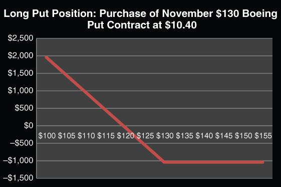
| Boeing Put on 3/25/2016: T = 11/18/16, X = $130, P = $10.40, Contract = 100 Puts; Boeing Stock = $132 | Return on Put | Return on Short Position on 100% Initial Margin | |
| Stock Price | Profit | Profit / ($10.40*100) | ($132 − ST)/ $132 |
| $100 | $1,960 | 188.46% | 24.24% |
| $105 | $1,460 | 140.38% | 20.45% |
| $110 | $960 | 92.31% | 16.67% |
| $115 | $460 | 44.23% | 12.88% |
| $120 | −$40 | −3.85% | 9.09% |
| $125 | −$540 | −51.92% | 5.30% |
| $130 | −$1,040 | −100.00% | 1.52% |
| $135 | −$1,040 | −100.00% | −2.27% |
| $140 | −$1,040 | −100.00% | −6.06% |
| $145 | −$1,040 | −100.00% | −9.85% |
| $150 | −$1,040 | −100.00% | −13.64% |
| $155 | −$1,040 | −100.00% | −17.42% |
| Break‐Even Price = $119.60 | |||
EXHIBIT 7.10 Put Purchase and Short Stock Position
Put Purchase Strategies
A put purchase strategy is used when the price of a stock is expected to decline. Bearish investors should keep two points in mind in selecting puts. First, an out‐of‐the‐money put provides a higher return‐risk investment than an in‐the‐money put. For example, suppose that ABC stock is at $59, an out‐of‐the‐money ABC June 55 put is trading at $1, and an in‐the‐money ABC June 60 put is at $3. If the price of ABC decreases to $50 near expiration, then the 55 put could be sold at its intrinsic value of $5, yielding a rate of return of 400% (($5 −$1)/$1), while the 60 put could be sold at its intrinsic value of $10 to yield a rate of 233% (($10 − $3)/$3). In contrast, if ABC drops to only $55, then the out‐of‐the‐money 55 put would be worthless, while the 60 put would yield a profit of $2 (at $60 or higher, both puts yield 100% losses). Thus, an out‐of‐the‐money put offers higher potential rewards but also higher risk than an in‐the‐money put. Second, it is important to keep in mind that in‐the‐money puts tend to lose their value faster than out‐of‐the‐money puts when the price of the stock increases. This is because when the price of the underlying stock increases over time, the in‐the‐money put loses both its intrinsic value and its time value premium, while the out‐of‐the‐money losses just its time value premium.
Follow‐Up Strategies
Once an investor has purchased a put, she needs to be able to identify the possible follow‐up actions that can be pursued if the stock price changes are different from what she expects. Aggressive follow‐up actions can be taken if the stock decreases more than expected, and defensive actions can be used if the stock increases in price.
Aggressive Follow‐Up Strategies
To see the types of aggressive strategies one can use, consider the case of an investor who purchased the Devon Energy, April 2016, 24 put contract for $1.94 on 1/29/16 when Devon was trading at $27.90. Exhibit 7.11 shows the Bloomberg price graphs for Devon Energy stock, its April 24 put, April 20 put, and April 26 put. As shown in the graph, the price of Devon decreased to $26.59 on 2/2/16, causing the April 24 put to increase to $2.72 and the April 20 put to increase to $1.34. Faced with this positive development, the Devon put buyer would have had a number of alternatives open to her. First, she could have liquidated by selling the 24 put for $2.72, realizing a profit of $78.00 (= ($2.72 − $1.94)(100)). The advantage of liquidating is certainty: The investor would know that even if the price of the stock increased, she will still have earned $78.00. The disadvantage of liquidating, of course, is the opportunity loss if the stock decreased in price. If the investor had strongly felt that Devon Energy would continue to decrease, then a second follow‐up strategy is to do nothing. As shown in Exhibit 7.12, if the stock reached $20 at expiration (T) then the investor would have realized a profit of $206 by selling the put at a price equal to its intrinsic value of $4.00—this is $128 more than if she had liquidated.

EXHIBIT 7.11 Price Graphs: Devon Energy, Devon April 24 Put, Devon April 20 Put, and Devon April 26 Put, 1/15/16 to 3/28/16
| Devon Energy: April 24 Put Contract purchased at $1.94 on 1/29/2016 when Stock was selling at $27.90 | ||||
| Stock Price at Expiration, 4/15/16 | Liquidate: Sell 24 Put for $2.72 on 2/2/16 | Do Nothing | Spread: 24 put Purchased at $1.94 on 1/15/16; 20 put Sold for $1.34 on 2/3/16 | Roll Down: Sell the 24 Put Contract for $2.72 and buy 2.03 April 20 put Contracts at $1.34 |
| $15.00 | $78 | $706 | $340 | $821 |
| $17.50 | $78 | $456 | $340 | $314 |
| $20.00 | $78 | $206 | $340 | −$194 |
| $22.50 | $78 | −$44 | $90 | −$194 |
| $25.00 | $78 | −$194 | −$60 | −$194 |
| $27.50 | $78 | −$194 | −$60 | −$194 |
| $30.00 | $78 | −$194 | −$60 | −$194 |
| $32.50 | $78 | −$194 | −$60 | −$194 |
| $35.00 | $78 | −$194 | −$60 | −$194 |
EXHIBIT 7.12 Aggressive Follow‐Up Strategies for April 24 Put Purchase
If the put purchaser wanted to gain more than just $206—in case the stock continues to decline—but did not want to lose if the stock increased, she could have followed up the put purchase strategy by creating a spread. In the case of aggressive follow‐up strategies, a spread often is created by selling a put with a lower exercise price. In terms of our example, suppose the investor sold the April 20 put contract for $1.34 when the stock was at $26.59. As shown in exhibit, at expiration the investor would realize a limited profit of $340 if the price of Devon were $20 or less and limited loss of $60 if the stock were $24 or greater, Thus, the spread would have yielded the investor less profit than the liquidating strategy if the stock price were to decrease, but unlike the do‐nothing strategy, the spread would lock in a smaller loss if the stock increased.
If, after the price of the stock reached $26.59, the expectation was that the price would continue to fall, then the investor might want to consider a roll‐down follow‐up strategy. This could have been done by selling the 24 put contracts for $272 and using the proceeds to buy 2.03 April 20 puts at $1.34 (assume perfect divisibility). This roll‐down strategy would have provided the investor with a relatively substantial gain near expiration if the stock were to have decreased in price, but also would have resulted in losses if the stock were to have increased. To minimize the range in potential profits and losses, the investor alternatively could have implemented a roll‐down strategy by selling the 24 puts and then using only the profit to buy 0.582 April 20 puts at 1.34.
Defensive Follow‐Up Strategies
If, after purchasing a put the price of the stock unexpectedly increases, an investor needs to consider defensive follow‐up strategies. For example, from 2/3/16 to 2/19/16, Devon Energy’s stock decreased from $26.59 to $18.65, the April 24 put increased from $2.72 to $6.06 and the April 20 put increased from $1.34 to $3.25. Suppose on 2/19/16 an investor bearish about Devon bought the April 24 put at $6.06. As shown in Exhibit 7.11, from 2/19/16 to 3/7/16, Devon increased from $18.65 to $24.19, causing the April 20 put to decrease from $6.06 to $2.22 and the April 20 put to fall from $3.25 to $0.71. Faced with this negative development, the put investor could have liquidated, incurring a loss of $384 (= ($2.22 − $6.06)(100)). This contrast to a $606 loss that he would have incurred if he did nothing and the price of the stock stayed above the $24 exercise price near expiration (see Exhibit 7.13). In contrast to this do‐nothing strategy, liquidating does eliminate potential profit if the stock price reverses itself. If the investor thought that the price increase was a signal of further price increases, he could have created a spread to minimize his losses (if the stock were to increase). As shown in Exhibit 7.13, if the holder combined the long position in the April 24 put with a short position in the April 26 put trading on 3/7/16 for 3.97, the investor would have limited his losses to $409 if the stock reached $24 or less at expiration. However, if the stock increased to $26 or higher, the investor would have lost only $209. Finally, if the investor believed Devon’s stock could go either up or down, he could have combined his put with a 24 call to form a straddle or sold the put and used the proceeds to buy a call.
| Stock Price at Expiration, 4/15/16 | Liquidate: Sell 24 Put for $2.22 on 3/7/16 | Do Nothing | Spread: April 24 Put Purchased at $6.06 on 2/19/16; April 26 Put Sold for $3.97 on 3/7/16 |
| $15.00 | −$384 | $294 | −$409 |
| $17.50 | −$384 | $44 | −$409 |
| $20.00 | −$384 | −$206 | −$409 |
| $22.50 | −$384 | −$456 | −$409 |
| $25.00 | −$384 | −$606 | −$309 |
| $27.50 | −$384 | −$606 | −$209 |
| $30.00 | −$384 | −$606 | −$209 |
| $32.50 | −$384 | −$606 | −$209 |
| $35.00 | −$384 | −$606 | −$209 |
EXHIBIT 7.13 Defensive Follow‐Up Strategies for April 24 Put Purchased at $6.06
Put Purchases in Conjunction with a Long Stock Position
Simulated Call
Purchasing a put and owning the underlying stock on a one‐to‐one basis, {+P, +S}, yields the same type of profit and stock price relation as a call purchase—simulated call. In Exhibit 7.14, the profits at expiration for various stock prices are shown for a long put and stock position consisting of 100 shares of Boeing stock purchased at $132 per share and an April 130 put contract purchased at $10.40. As can be seen in the table and the accompanying figure in the exhibit, the combined put and stock position yields the same relation as the purchase of a 130 April call contract at $12.40. Note, however, that more often than not, calls and puts with identical terms are not likely to be equally priced. To form an identical long call position with a call price consistent with put‐call parity, a synthetic call, requires not only buying the put and stock, but also shorting a bond with a face value equal to the exercise price (i.e., borrow an amount equal to the present value of exercise price: PV(X) = B0):
or as

| Boeing Put on 3/25/2016: T =11/18/16, X = $130, P = $10.40, Contract = 100 Puts; Boeing Stock = $132 |
|||
| Stock Price | Put Profit = Max(0, $130 − ST) − $10.40)100 | Stock Profit = (ST − $132)100 | Total Profit |
| $100 | $1,960 | −$3,200 | −$1,240 |
| $105 | $1,460 | −$2,700 | −$1,240 |
| $110 | $960 | −$2,200 | −$1,240 |
| $115 | $460 | −$1,700 | −$1,240 |
| $120 | −$40 | −$1,200 | −$1,240 |
| $125 | −$540 | −$700 | −$1,240 |
| $130 | −$1,040 | −$200 | −$1,240 |
| $135 | −$1,040 | $300 | −$740 |
| $140 | −$1,040 | $800 | −$240 |
| $145 | −$1,040 | $1,300 | $260 |
| $150 | −$1,040 | $1,800 | $760 |
| $155 | −$1,040 | $2,300 | $1,260 |
| $160 | −$1,040 | $2,800 | $1,760 |
| $165 | −$1,040 | $3,300 | $2,260 |
EXHIBIT 7.14 Long Stock and Put Position Simulated Call and Stock Insurance
Portfolio Insurance
As we discussed in Chapter 5, the combined stock and put position is known as a portfolio insurance or stock insurance strategy. The features of such a strategy are best seen by examining the position’s cash flows and value graph, shown in the table and figure in Exhibit 7.15. As shown, the 130 Boeing put provides downside protection against the stock falling below $130, while allowing for the upside profit potential if the stock increases. Thus, for the cost of the put premium of $1,040, an investor can obtain insurance against decreases in the stock’s price. Hedging a stock portfolio positions with index put options is a popular hedging strategy used by portfolio managers. Portfolio insurance using index options are examined in more detail in Chapter 8.

| Boeing Put on 3/25/2016: T = 11/18/16, X = $130, P = $10.40, Contract = 100 Puts; Boeing Stock = $132 |
|||
| Stock Price | Stock Value = ST 100 | Put Value = Max($130 − ST, 0)100 | Hedged Stock Value = Stock Value + Put Value |
| $100 | $10,000 | $3,000 | $13,000 |
| $105 | $10,500 | $2,500 | $13,000 |
| $110 | $11,000 | $2,000 | $13,000 |
| $115 | $11,500 | $1,500 | $13,000 |
| $120 | $12,000 | $1,000 | $13,000 |
| $125 | $12,500 | $500 | $13,000 |
| $130 | $13,000 | $0 | $13,000 |
| $135 | $13,500 | $0 | $13,500 |
| $140 | $14,000 | $0 | $14,000 |
| $145 | $14,500 | $0 | $14,500 |
| $150 | $15,000 | $0 | $15,000 |
| $155 | $15,500 | $0 | $15,500 |
EXHIBIT 7.15 Value Graph and Table of Long Stock and Put Positions: Stock Insurance
Naked Put Writes
The naked (or uncovered) put write strategy provides only limited profit potential if the stock price increases with the chances of large losses if the stock price decreases. The position as defined in terms of its profit and stock price relationship near expiration is equivalent (though not identical) to the covered call write. Besides being similar to the covered call write, the naked put write strategy also is like the naked call write in that it provides an opportunity for investors to profit from the decrease over time in the option’s time value premium. For example, the Boeing April $130 put selling in March for $10.40 when Boeing stock was trading at $132 would, with no change in the stock price, trade at its intrinsic value of $2.00 at expiration. Thus, a profit of $8.40 would have been earned by the naked put writer from the decrease in the time value premium.
Similar to the naked call write, naked put write strategies with in‐the‐money puts provide higher return‐risk combinations than those with out‐of‐the‐money puts. Thus, the more the put is in the money, the greater return‐risk possibilities (at expiration) available from a naked put write position.
Finally, the defensive rolling credit follow‐up strategy defined for the naked call write position can be applied to the naked put write strategy for cases in which the stock decreases in price. For example, if Boeing stock decreased from $132 to $130, causing the April 130 put to go from $10.40 to $12.30, the writer of the April 130 put could roll down by selling, say, Boeing April 128 puts, and then using the proceeds (or credit) to close the April 130 puts. Like the rolling credit strategy for the uncovered call write position, this strategy needs to be repeated each time the stock decreases to a new, uncomfortable level. In turn, the put writer will profit from this follow‐up strategy provided the stock eventually stops decreasing, the option is not exercised, and the writer has sufficient collateral to cover each follow‐up adjustment.
Covered Put Writes
The covered put write strategy involves selling a put and shorting the underlying stock: {−P, −S}. It is equivalent (but not identical) to the naked call write, providing limited profit potential if the stock declines and unlimited loss possibilities if the price of the stock increases. The naked call write, however, has a smaller commission cost and lower collateral requirements than the covered put write. As a short‐run speculative strategy, the covered put write is not as good as the naked call write and, as such, is seldom used as a strategy by option traders.
Analogous to a covered call write, a covered put write can be used as a hedging strategy for a short stock position or as a way of increasing returns for an investor who is short in the stock. For example, an investor who was short in Boeing stock at $132 and was worried about an increase in the price of the stock above $132 could offset some of the losses resulting from a stock price increase by selling a put option on Boeing. The premium received from the put sale would then serve to partially offset losses on the short positions if the stock increased. If the stock decreased, though, then the short seller would find her profits from her short position offset by losses on her short put position.
Ratio Put Writes
The ratio put write is a combination of a covered put write and a naked put write. It is formed by selling puts against shares of stock shorted at a ratio different than 1:1, for example, selling two puts for each share of stock shorted: {−2P, −S}. In terms of its profit and stock price relationship near expiration, the ratio put write is equivalent to the ratio call write. Like the ratio call write, the ratio put position is characterized by an inverted V‐shaped profit and stock relation, two break‐even prices, and a maximum profit occurring when the stock price is equal to the exercise price. The major difference between these equivalent strategies is that the ratio call write requires an investment to purchase the stock, while the ratio put write requires posting collateral to cover the short sale.
The ratio put write position can be reversed. This strategy is known as a reverse hedge with puts. The strategy yields a V‐shaped profit and stock price relation and is equivalent to the straddle purchase.
Call Spreads
As discussed in Chapter 5, a call spread is a strategy in which one simultaneously buys one call option and sells another on the same stock but with different terms. There are three types of spreads:
- The vertical (or money or price) spread, in which the options have the same expiration dates but different exercise prices
- The horizontal (or time or calendar) spread, in which the options have the same exercise price but different expiration dates
- The diagonal spread, which combines the vertical and horizontal spreads by having options with both different exercise prices and expiration dates
Vertical (Money) Spreads
The most popular vertical or money spreads are the bull, bear, ratio, and butterfly spreads.
Bull and Bear Call Spreads
The bull money call spread is suited for investors who are bullish about a security. The strategy is formed by going long in a call with a given exercise price and short in another call on the same underlying security with a higher exercise price. For example, on 5/20/16 the S&P 500 was at 2,040, an August S&P 500 2,030 call was trading at 70.20, and an August S&P 500 2,050 call was trading at 57.60 ($100 multiplier). To form a bull spread on those S&P 500 calls, a spreader would have bought the 2,030 call and sold the 2,050 calls: {+C(2,030), −C(2,050)}. As shown in Exhibit 7.16, this bull money spread is characterized by losses limited to $1,260 if the S&P 500 was trading at 2,030 (the low exercise price) or less at expiration, and limited profits of $740, if the S&P were trading at 2,050 (the high exercise price) or higher at expiration.

| S&P 500 Call Spread: August 2,030 Call Trading at 70.20 August 2,050 Call Trading at 57.50; Multiplier = 100 |
|||
| S&P 500 Index, ST | Long 2030 Call: {Max(ST − 2,030,0) −70.20}(100) | Short 2050 Call: {−Max(ST − 2,050,0) + 57.60}(100) | Total Profit |
| 1,970 | −$7,020 | $5,760 | −$1,260 |
| 1,990 | −$7,020 | $5,760 | −$1,260 |
| 2,010 | −$7,020 | $5,760 | −$1,260 |
| 2,030 | −$7,020 | $5,760 | −$1,260 |
| 2,050 | −$5,020 | $5,760 | $740 |
| 2,070 | −$3,020 | $3,760 | $740 |
| 2,090 | −$1,020 | $1,760 | $740 |
| 2,110 | $980 | −$240 | $740 |
EXHIBIT 7.16 Bull Call Spread
The bear money call spread is the exact opposite of the bull spread. It is formed by buying a call at a specific exercise price and selling a call on the same stock but with a lower strike price. In terms of the previous example, if the spreader bought the S&P 500 2,050 call at $57.60 and sold the 2,030 call at 70.20: {+C(2,050), −C(2,030)}, then as shown in Exhibit 7.17 and its accompanying figure, her profit would be limited to $1,260 if the S&P 500 were $2,030 or less, and her loss would be $740 if the S&P 500 were $2,050 or higher.

| S&P 500 Call Spread: August 2,030 Call Trading at 70.20 August 2,050 Call Trading at 57.50; Multiplier = 100 |
|||
| S&P 500 Index, ST | Short 2030 Call: {−Max(ST −2,030,0) + 70.20}(100) | Long in 2050 Call: {Max(ST − 2050, 0) − 57.60}(100) | Total Profit |
| 1,970 | $7,020 | −$5,760 | $1,260 |
| 1,990 | $7,020 | −$5,760 | $1,260 |
| 2,010 | $7,020 | −$5,760 | $1,260 |
| 2,030 | $7,020 | −$5,760 | $1,260 |
| 2,050 | $5,020 | −$5,760 | −$740 |
| 2,070 | $3,020 | −$3,760 | −$740 |
| 2,090 | $1,020 | −$1,760 | −$740 |
| 2,110 | −$980 | $240 | −$740 |
EXHIBIT 7.17 Bear Call Spread
Ratio Money Spreads
The bull and bear spreads are balanced spreads or 1:1 money spreads. A ratio money spread, in turn, is formed by taking long and short positions in options that have not only different exercise prices but also ratios different than 1:1. The ratio money spread can be formed, for example, either by taking a long position in the low exercise call and a short position in the high one in different ratios, or by going short in the low exercise call and long in the high one in different ratios. For a given ratio, these two spreads yield exactly opposite results.
Using the previous example, a ratio money spread could be formed by buying one August S&P 500 2,030 call at 70.20 and selling two August S&P 500 2,050 calls at 57.60: {+C(2,030), −2C(2,050)}. As shown in Exhibit 7.18, this 1:2 ratio money spread is characterized by a limited profit of $4,500 if the S&P 500 is at the exercise price of 2,030 or less, profit increasing from $4,500 at 2,030 to $6,500 at 2,050, and then decreasing profit and losses occurring if the S&P 500 declines from 2,050. Hence, the motivation for this strategy would be if an investor expected the market to go to 2,050 or decline.

| S&P 500 Call Spread: August 2,030 Call Trading at 70.20 August 2,050 Call Trading at 57.50; Multiplier = 100 |
|||
| 1 | 2 | 3 | 4 |
| S&P 500 Index, ST | Bear Spread | 1:2 Ratio Spread | 1:3 Ratio Spread |
| 1,970 | $1,260 | $4,500 | $10,260 |
| 1,990 | $1,260 | $4,500 | $10,260 |
| 2,010 | $1,260 | $4,500 | $10,260 |
| 2,030 | $1,260 | $4,500 | $10,260 |
| 2,050 | −$740 | $6,500 | $12,260 |
| 2,070 | −$740 | $4,500 | $8,260 |
| 2,090 | −$740 | $2,500 | $4,260 |
| 2,110 | −$740 | $500 | $260 |
| 2,130 | −$740 | −$1,500 | −$3,740 |
| 2,150 | −$740 | −$3,500 | −$7,740 |
| 2,170 | −$740 | −$5,500 | −$11,740 |
EXHIBIT 7.18 Ratio Call Spreads and Bear Money Spreads
In general, the characteristics of the money spread can be varied by changing the spread’s ratio. This can be seen by comparing the profit and S&P 500 index relations for the 1:2 money spread with the 1:3 spread in which the profit hits a maximum of $12,260 when the S&P 500 is at 2,050, stabilizes at a profit of $10,260 when the index is at 2,030 or less, and declines if the index declines from 2,050. This ratio money spreads would be an alternative for a bearish investor to the bear spread. The profit graphs of the three spreads are shown in Exhibit 7.18.
Butterfly Money Spreads
The butterfly spread (also referred to as the sandwich spread) is a combination of the bull and bear spreads. Specifically, a long butterfly money call spread is formed by buying one call at a low exercise price, selling two calls at a middle exercise price, and buying one call at a high exercise price. To see the profit and stock price relations that a long butterfly generates, consider a spread formed with the Philadelphia Stock Exchange Gold & Silver Index (XAU): an index that includes the leading companies involved in the mining of gold and silver. On May 24, 2016, the XAU index was at 85.10, the August 70 XAU call was trading at 19.20, the August XAU 85 call was at 10.00, and the August XAU 100 call was at 4.70 (multiplier = $100). Suppose an investor formed a butterfly spread with these call options: long in one 70 call, short in two 85 calls, and long in one 100 call: {+C(70), −2C(85), +C(100)}. As shown in Exhibit 7.19, this long butterfly spread would generate an inverted V‐shaped profit and index price relation, with limited losses at high and low index prices. The maximum profit of $1,100 occurs when the index equals the middle exercise price of 85 and the limited losses of $390 start when the index price is equal to the high (100) and low (70) exercise prices. The long butterfly money spread is, in turn, a strategy that can be used if one expects the index to be near the middle exercise price near expiration. The long butterfly spread is an alternative to a short straddle. Compared to the short straddle formed with call and puts with the middle exercise price (e.g., 85), the butterfly provides limited losses, but lower maximum profit. See Exhibit 7.19.
| Philadelphia Stock Exhange Gold & Silver Index, AUX AUX 70 Call Trading at 19.20; AUX 85 Call Trading at 10; AUX 100 Call Trading at 4.70; AUX 85 Put Trading at 7.70 |
|||||||
| 1 | 2 | 3 | 4 | 5 | 6 | 7 | 8 |
| Philadelphia Stock Exhange Gold & Silver Index, AUX | Long One 70 AUX Call: {(Max(ST − 70,0) − 19.20}(100) | Short Two 85 AUX Calls: 2{−(Max(ST − 85, 0) + 10}(100) | Long One 100 AUX Call: {(Max(ST −100),0) − 4.70}(100) | Long Butterfly Col(2) + Col(3) + Col(4) | Short One 85 AUX Call: {Max(ST − 85,0) − 10}(100) | Short One 85 AUX Put: {Max(85 − ST,0) − 7.70}(100) | Short 85 Straddle |
| 45 | −$1,920 | $2,000 | −$470 | −$390 | $1,000 | −$3,230 | −$2,230 |
| 50 | −$1,920 | $2,000 | −$470 | −$390 | $1,000 | −$2,730 | −$1,730 |
| 55 | −$1,920 | $2,000 | −$470 | −$390 | $1,000 | −$2,230 | −$1,230 |
| 60 | −$1,920 | $2,000 | −$470 | −$390 | $1,000 | −$1,730 | −$730 |
| 65 | −$1,920 | $2,000 | −$470 | −$390 | $1,000 | −$1,230 | −$230 |
| 70 | −$1,920 | $2,000 | −$470 | −$390 | $1,000 | −$730 | $270 |
| 75 | −$1,420 | $2,000 | −$470 | $110 | $1,000 | −$230 | $770 |
| 80 | −$920 | $2,000 | −$470 | $610 | $1,000 | $270 | $1,270 |
| 85 | −$420 | $2,000 | −$470 | $1,110 | $1,000 | $770 | $1,770 |
| 90 | $80 | $1,000 | −$470 | $610 | $500 | $770 | $1,270 |
| 95 | $580 | $0 | −$470 | $110 | $0 | $770 | $770 |
| 100 | $1,080 | −$1,000 | −$470 | −$390 | −$500 | $770 | $270 |
| 105 | $1,580 | −$2,000 | $30 | −$390 | −$1,000 | $770 | −$230 |
| 110 | $2,080 | −$3,000 | $530 | −$390 | −$1,500 | $770 | −$730 |
| 115 | $2,580 | −$4,000 | $1,030 | −$390 | −$2,000 | $770 | −$1,230 |
| 120 | $3,080 | −$5,000 | $1,530 | −$390 | −$2,500 | $770 | −$1,730 |
| 125 | $3,580 | −$6,000 | $2,030 | −$390 | −$3,000 | $770 | −$2,230 |

EXHIBIT 7.19 Long Butterfly Spread and Short Straddle
A short butterfly money call spread is the exact opposite of the long butterfly. It is formed by selling a low exercise call, buying two middle exercise calls, and selling a high exercise call. Exhibit 7.20 illustrates the profit and stock price relations for the short butterfly spread formed by going short in one 70 XAU call, long in two XAU 85 calls, and short in one XAU 100 call: {−C(70), +2C(85), −C(100)}. As shown in the graph, the short butterfly yields a V‐shaped profit and security price relation with limited profits starting when the underlying security price is at the high and low exercise prices. The short butterfly spread is an alternative to a long straddle. Compared to a long straddle formed with call and puts with the middle exercise price (e.g., 85), the short butterfly provides limited profits, but a lower minimum loss.
| Philadelphia Stock Exhange Gold & Silver Index, AUX AUX 70 Call Trading at 19.20; AUX 85 Call Trading at 10; AUX 100 Call Trading at 4.70; AUX 85 Put Trading at 7.70 |
|||||||
| 1 | 2 | 3 | 4 | 5 | 6 | 7 | 8 |
| Philadelphia Stock Exhange Gold & Silver Index, AUX | Short One 70 AUX Call: {−(Max(ST − 70,0) + 19.20}(100) | Long Two 85 AUX Calls: 2{(Max(ST − 85,0) − 10}(100) | Short One 100 AUX Call: {−(Max(ST −100),0) + 4.70}(100) | Short Butterfly Col(2) + Col(3) + Col(4) | Long One 85 AUX Call: {Max(ST − 85,0) − 10}(100) | Long One 85 AUX Put: {Max(85 − ST,0) − 7.70}(100) | Long 85 Straddle |
| 45 | $1,920 | −$2,000 | $470 | $390 | −$1,000 | $3,230 | $2,230 |
| 50 | $1,920 | −$2,000 | $470 | $390 | −$1,000 | $2,730 | $1,730 |
| 55 | $1,920 | −$2,000 | $470 | $390 | −$1,000 | $2,230 | $1,230 |
| 60 | $1,920 | −$2,000 | $470 | $390 | −$1,000 | $1,730 | $730 |
| 65 | $1,920 | −$2,000 | $470 | $390 | −$1,000 | $1,230 | $230 |
| 70 | $1,920 | −$2,000 | $470 | $390 | −$1,000 | $730 | −$270 |
| 75 | $1,420 | −$2,000 | $470 | −$110 | −$1,000 | $230 | −$770 |
| 80 | $920 | −$2,000 | $470 | −$610 | −$1,000 | −$270 | −$1,270 |
| 85 | $420 | −$2,000 | $470 | −$1,110 | −$1,000 | −$770 | −$1,770 |
| 90 | −$80 | −$1,000 | $470 | −$610 | −$500 | −$770 | −$1,270 |
| 95 | −$580 | $0 | $470 | −$110 | $0 | −$770 | −$770 |
| 100 | −$1,080 | $1,000 | $470 | $390 | $500 | −$770 | −$270 |
| 105 | −$1,580 | $2,000 | −$30 | $390 | $1,000 | −$770 | $230 |
| 110 | −$2,080 | $3,000 | −$530 | $390 | $1,500 | −$770 | $730 |
| 115 | −$2,580 | $4,000 | −$1,030 | $390 | $2,000 | −$770 | $1,230 |
| 120 | −$3,080 | $5,000 | −$1,530 | $390 | $2,500 | −$770 | $1,730 |
| 125 | −$3,580 | $6,000 | −$2,030 | $390 | $3,000 | −$770 | $2,230 |

EXHIBIT 7.20 Short Butterfly Spread and Long Straddle
Horizontal (Time) Spreads
The horizontal (or time or calendar) spread is formed by simultaneously buying and selling options that are identical except for the time to expiration. For example, a horizontal spread could be formed by selling an ABC June 50 call at $5 and buying a September 50 call at $9. A number of different types of time spreads exist. For example, a spreader may want to form a ratio time spread by going long in one long‐term call and short in two short‐term calls. An option investor also could form a butterfly time spread with three options with the same exercise prices but with different exercise dates.
Since horizontal, as well as diagonal, spreads have different exercise dates, it is impossible to know with certainty the value of the long‐term option position at the expiration date of the short‐term option position. As a result, time and diagonal spreads do not lend themselves to the same type of profit and security price analysis associated with the strategies we have analyzed to this point. We can, however, estimate profit and stock price relations by using the option pricing model to estimate the price of the longer‐term option for each possible stock price at the expiration of the shorter‐term one. We will discuss time and diagonal spreads following our examination of option pricing models.
Put Spreads
Horizontal, vertical, and diagonal put spreads are formed the same way as their corresponding call spreads, and they produce the same profit and stock price relation as their corresponding call spreads. For example, a call bear spread is formed by selling a call with a lower exercise price and buying one with a higher, and a put bear spread is also formed by selling a low exercise put and buying a higher exercise one. Both strategies yield the same profit and stock price relation. Similarly, a calendar put spread is constructed like its corresponding call by buying (or selling) a short‐term put and selling (buying) a longer‐term one.
In general, our preceding discussion on call spreads also applies to put spreads. It should be kept in mind that even though the put and call spreads are equivalent in terms of profit and stock price relation, differences do exist. For instance, with a bear put spread, the higher exercise price put will sell for more than the lower exercise one, leading to a debit position. The bear call spread, however, will have a higher premium associated with its lower exercise price option and a lower premium associated with its higher exercise call, thus leading to an initial credit position. In contrast, the bull put spread will yield a net credit position and the bull call spread a net debit one. Also, in comparing equivalent call and put spreads, it is important to note that the time value premium for puts may respond differently to stock price changes than do the time premiums for calls, thus leading to different uses of calendar put and calendar call spread strategies.
Straddle, Strip, and Strap Positions
The straddle is one of the more well‐known option strategies. As previously described, a straddle purchase is formed by buying both a put and a call with the same terms—same underlying security, exercise price, and expiration date: {+C, +P}. A straddle write, in contrast, is formed by selling a call and a put with the same terms: {−C, −P}. For the straddle positions, the ratio of calls to puts is 1:1. Changing the ratio, in turn, yields either a strip or strap option strategy. Specifically, the strip is formed by having more puts than calls, and the strap is constructed with more calls than puts.
Straddle Purchases
The straddle purchase yields a V‐shaped profit and security price relation near expiration with two break‐even prices and the maximum loss equal to the sum of the call and put premium that occurs when the security is equal to the options’ exercise price. In Exhibit 7.20, Columns (6), (7), and (8), the profit and index relation is shown for a straddle purchase consisting of an AUX August 85 call purchased for $10 and the August 85 put bought for $7.70.
The straddle purchase (or long straddle) is equivalent to the simulated straddle and the reverse hedge strategy. Since the simulated straddle and reverse hedge strategies involve security positions, they have the disadvantage of higher commission cost compared to the straddle purchase. Thus, the straddle purchase is the preferable short‐run strategy.
The straddle purchase, as with all strategies that are characterized by V‐shaped profit and security price relations, is well‐suited for cases in which an investor expects substantial change in the price of the stock to occur but is not sure whether the change will be positive or negative. Although all long straddles are characterized by V‐shaped profit graphs, different straddles on the same stock—differing in terms of their maximum loss, their break‐even prices, and the rate of change in profits per change in stock prices (i.e., slopes)—can be generated by purchasing either an out‐of‐the‐money call and in‐the‐money put, an out/in (call/put) straddle, or an in/out straddle.
Since many straddle strategies are based on anticipated events that could occur before the options’ expiration date, they lend themselves to follow‐up actions. As an example, suppose that when the Philadelphia Gold & Silver Index was at 85, an investor purchased the 85 AUX straddle. Then suppose that after the straddle was purchased, but before the options expired, leading economic indicators were released that augured for an economic slowdown, causing the Philadelphia Gold & Silver Index to increase, the AUX 85 call to increase, and the AUX 85 put to decrease. Given this new situation, the investor could: (1) liquidate, if he felt the index was at a maximum and would stay there; (2) sell the call and keep the put, if he believed the market overreacted to the announcement and that therefore the index would decline; (3) sell the put and hold the call, if he believed the index would increase even further; or (4) roll‐up the call (put) by liquidating the straddle and using the profit to buy AUX calls (put) with higher exercise prices. As always, determining what follow‐up strategy to choose depends on the investor’s expectation after an event and his confidence in his expectation.
Straddle Writes
The straddle write (or short straddle) yields an inverted V‐shaped profit and security price relation near expiration, with two break‐even prices and a maximum profit equal to the sum of the call and put premiums occurring when the price of the stock is equal to the options’ exercise price. The short straddle is equivalent to the ratio call write strategy, discussed earlier. In Exhibit 7.19, Columns (6), (7), and (8), the profit and index price relation is shown for a straddle sale consisting of an AUX August 85 call sold for $10 and an AUG August put sold for $7.70.
The straddle write and other equivalent strategies yielding inverted V‐shaped profit graphs are ideal for cases in which one either expects little change to occur in the price of the security, or, given the security’s variability, is confident the price of the stock will fall within the range of the break‐even prices. Thus, in contrast to the straddle purchaser, the straddle writer does not anticipate an event occurring in the near term that would affect the price of the underlying stock.
If an event does occur that increases or decreases the stock price, the writer may need to consider defensive follow‐up action. For example, in our previous case in which the Philadelphia Gold & Silver Index increased, a straddle writer who sold the straddle expecting little changes could consider liquidating the short straddle, thus limiting his losses, possibly closing the call by buying it back, or closing the put position. A number of strategies, both defensive and aggressive, can be employed, including positions with different exercise prices and exercise dates.
Strips and Straps
Strips and straps are variations of the straddle. They are formed by adding an additional call position (strap) or an additional put position (strip) to a straddle. Specifically, the strip purchase (sale) consists of the long (short) straddle position plus the purchase (sale) of an extra put(s); the strap purchase (sale) consists of the long (short) straddle plus the additional purchase (sale) of a call(s). In Exhibit 7.21, the profit and index price relations for long straddle, strip, and strap positions formed with an AUX 85 call trading at $10 and an AUX 85 put trading for $7.70 are shown. In Exhibit 7.22, the short positions for the strip, strap, and straddle formed with the same options are shown.

| Philadelphia Stock Exhange Gold & Silver Index, AUX AUX 85 Call Trading at 10; AUX 85 Put Trading at 7.70 |
|||
| Philadelphia Stock Exhange Gold & Silver Index, AUX | Straddle: Long One 85 AUX Call and One AUX 85 Put | Strap: Long Two 85 AUX Calls and One 85 AUX Put | Strip: Long Two 85 AUX Puts and One 85 AUX Call |
| 40 | $2,730 | $1,730 | $6,460 |
| 45 | $2,230 | $1,230 | $5,460 |
| 50 | $1,730 | $730 | $4,460 |
| 55 | $1,230 | $230 | $3,460 |
| 60 | $730 | −$270 | $2,460 |
| 65 | $230 | −$770 | $1,460 |
| 70 | −$270 | −$1,270 | $460 |
| 75 | −$770 | −$1,770 | −$540 |
| 80 | −$1,270 | −$2,270 | −$1,540 |
| 85 | −$1,770 | −$2,770 | −$2,540 |
| 90 | −$1,270 | −$1,770 | −$2,040 |
| 95 | −$770 | −$770 | −$1,540 |
| 100 | −$270 | $230 | −$1,040 |
| 105 | $230 | $1,230 | −$540 |
| 110 | $730 | $2,230 | −$40 |
| 115 | $1,230 | $3,230 | $460 |
| 120 | $1,730 | $4,230 | $960 |
| 125 | $2,230 | $5,230 | $1,460 |
| 130 | $2,730 | $6,230 | $1,960 |
EXHIBIT 7.21 Long Straddle, Strip, and Strap

| Philadelphia Stock Exhange Gold & Silver Index, AUX AUX 85 Call Trading at 10; AUX 85 Put Trading at 7.70 |
|||
| Philadelphia Stock Exhange Gold & Silver Index, AUX | Straddle: Short One 85 AUX Call and One AUX 85 Put | Strap: Short Two 85 AUX Calls and One 85 AUX Put | Strip: Short Two 85 AUX Puts and One 85 AUX Call |
| 40 | −$2,730 | −$1,730 | −$6,460 |
| 45 | −$2,230 | −$1,230 | −$5,460 |
| 50 | −$1,730 | −$730 | −$4,460 |
| 55 | −$1,230 | −$230 | −$3,460 |
| 60 | −$730 | $270 | −$2,460 |
| 65 | −$230 | $770 | −$1,460 |
| 70 | $270 | $1,270 | −$460 |
| 75 | $770 | $1,770 | $540 |
| 80 | $1,270 | $2,270 | $1,540 |
| 85 | $1,770 | $2,770 | $2,540 |
| 90 | $1,270 | $1,770 | $2,040 |
| 95 | $770 | $770 | $1,540 |
| 100 | $270 | −$230 | $1,040 |
| 105 | −$230 | −$1,230 | $540 |
| 110 | −$730 | −$2,230 | $40 |
| 115 | −$1,230 | −$3,230 | −$460 |
| 120 | −$1,730 | −$4,230 | −$960 |
| 125 | −$2,230 | −$5,230 | −$1,460 |
| 130 | −$2,730 | −$6,230 | −$1,960 |
EXHIBIT 7.22 Short Straddle, Strip, and Strap
In comparing the three long positions, a number of differences should be noted. First, as we move from the straddle to the strip the break‐even prices move up, and as we move from the straddle to the strap, the break‐even prices move down. Secondly, compared to the symmetrical returns on the straddle, the strip and strap positions provide asymmetrical payoffs. The strip’s rate of increase in profit exceeds that of the straddle when the stock decreases from its maximum‐loss price and equals the straddle’s rate when the stock increases. Thus, a strip is particularly well‐suited for cases in which (like a straddle) an investor expects a stock either to increase or decrease in response to an event, but also expects that the stock response if the event is negative will be greater than its response if the event is positive. A strap, on the other hand, has a greater rate of increase in profit than the straddle when the stock increases and the same rate when the stock decreases.
Comparing the three short positions in Exhibit 7.22, the writer obtains wider ranges in the break‐even prices and a greater maximum profit from selling a strip and strap than a straddle. A strip’s losses, however, increase at a greater rate than a straddle write’s losses when the stock price decreases from the maximum profit price and at the same rate when the stock increases. The opposite results occur in the case of the strap write.
Finally, note that the characteristics of strips and straps can be changed by varying the ratios. This is illustrated in Exhibit 7.23, in which the long strap position with a 2:1 call‐to‐put ratio is compared to a 3:1 strip.

EXHIBIT 7.23 Straps with Different Ratios
Combinations
A combination is a position formed with a call and a put on the same underlying stock but with different terms: that is, either different exercise prices (referred to as a money or a vertical combination), exercise dates (called a time, calendar, or horizontal combination), or both (diagonal combination). The most common combinations are the ones formed with different exercise prices—money combinations, often called strangles.
In Exhibit 7.24, the profit and index price relations are shown for a long money combination (a long strangle) constructed with a December $1.11 euro futures call contract trading at $0.0297/€ on 9/1/16 and a December $1.15 euro futures put contract trading at $0.0379/€ (contract size = 125,000 euros) on 9/1/16. When the underlying December euro futures trading at $1.12425/€ on 9/1/16 the long combination consists of an in‐the‐money call and an in‐of‐the‐money put; that is, a 1.11/1.15 (call/put), in/in combination. As shown, the combination position is characterized by a limited loss $3,450 over a range of futures prices between the exercises prices ($1.11 and $1.15), and virtually unlimited profit potential if the underlying futures price increases or decreases. Short money combinations yield just the opposite—limited profit over a range of underlying security prices and potential losses if the underlying price changes substantially in either direction. In Exhibit 7.25, the profit and futures price relations are shown for a short money combination (a short strangle) constructed with the $1.11 December euro futures call and $1.15 euro futures put. Like straddles, different combinations on the same underlying security can be formed with in‐the‐money and out‐of‐the‐money calls and puts: out/in (call/put), in/out, and out/out combinations.

| CME Euro Futures Options Combination $1.11 December Futures Euro Call Trading at $0.0297 $1.15 December Futures Put Trading at $0.0379 December Futures Trading at $1.12425 on 9/1/2106 Long One $1.11 December Euro Futures Call: Profit{(Max(fT − $1.11),0) − $0.0297}(125,000) Long One $1.15 December Euro Futures Put: Profit {(Max($1.15 − fT),0) − $0.0379}(125,000) |
|||
| Profit: Long $1.11 Profit: Long $1.15 December Futures December Futures |
|||
| Euro Futures, fT | Call | Put | Long Combination: Total Profit |
| $1.07 | −$3,713 | $5,262 | $1,550 |
| $1.08 | −$3,713 | $4,012 | $300 |
| $1.09 | −$3,713 | $2,762 | −$950 |
| $1.10 | −$3,713 | $1,512 | −$2,200 |
| $1.11 | −$3,713 | $262 | −$3,450 |
| $1.12 | −$2,463 | −$988 | −$3,450 |
| $1.13 | −$1,213 | −$2,238 | −$3,450 |
| $1.14 | $37 | −$3,488 | −$3,450 |
| $1.15 | $1,287 | −$4,738 | −$3,450 |
| $1.16 | $2,537 | −$4,738 | −$2,200 |
| $1.17 | $3,787 | −$4,738 | −$950 |
| $1.18 | $5,037 | −$4,738 | $300 |
| $1.19 | $6,287 | −$4,738 | $1,550 |
EXHIBIT 7.24 Long Combination

| CME Euro Futures Options Combination $1.11 December Futures Euro Call Trading at $0.0297 $1.15 December Futures Put Trading at $0.0379 December Futures Trading at $1.12425 on 9/1/2106 Short One $1.11 December Euro Futures Call: Profit{$0.0297 − (Max(fT − $1.11),0)}(125,000) Short One $1.15 December Euro Futures Put: Profit{$0.0397 − (Max($1.15 − fT),0)}(125,000) |
|||
| Euro Futures, fT | Profit: Short $1.11 December Futures Call | Profit: Short $1.15 December Futures Put | Short Combination: Total Profit |
| $1.07 | $3,713 | −$5,262 | −$1,550 |
| $1.08 | $3,713 | −$4,012 | −$300 |
| $1.09 | $3,713 | −$2,762 | $950 |
| $1.10 | $3,713 | −$1,512 | $2,200 |
| $1.11 | $3,713 | −$262 | $3,450 |
| $1.12 | $2,463 | $988 | $3,450 |
| $1.13 | $1,213 | $2,238 | $3,450 |
| $1.14 | −$37 | $3,488 | $3,450 |
| $1.15 | −$1,287 | $4,738 | $3,450 |
| $1.16 | −$2,537 | $4,738 | $2,200 |
| $1.17 | −$3,787 | $4,738 | $950 |
| $1.18 | −$5,037 | $4,738 | −$300 |
| $1.19 | −$6,287 | $4,738 | −$1,550 |
EXHIBIT 7.25 Short Combination
Condors
Condors are formed with four call and/or put options on the same security but with different terms. They are a special type of butterfly spread involving bull and bear spreads with different exercise prices. Condors can be constructed in a number of ways. Exhibit 7.26 shows several ways in which a long condor can be formed with call and put options with four exercise prices: X1, X2, X3, and X4, in which X1 < X2 < X3 < X4. The long condor is similar to a short money combination, providing limited profit over a range of stock prices, and possible losses if the stock price changes in either direction. Different from the combination, the losses on the long condor are limited. This limited loss feature, in turn, makes the condor less risky than the combination. A short condor position is formed by simply reversing the long condor’s positions. The short condor, in turn, has the opposite characteristics of the long position.
| Long Condor | |
| Calls: | Long X1 and X4; Short X2 and X3 |
| Puts: | Long X1 and X4; Short X2 and X3 |
| Calls and Puts: | Long X1 Call, Short X2 Call, Short X3 Put, Long X4 Put |
| Calls and Puts: | Long X1 Put, Short X2 Put, Short X3 Call, Long X4 Call |
| Short Condor | |
| Calls: | Short X1 and X4; Long X2 and X3 |
| Puts: | Short X1 and X4; Long X2 and X3 |
| Calls and Puts: | Short X1 Call, Long X2 Call, Long X3 Put, Short X4 Put |
| Calls and Puts: | Short X1 Put, Long X2 Put, Long X3 Call, Short X4 Call |
EXHIBIT 7.26 Condors
Simulated Stock Positions
Given that options can be used in different combinations to obtain virtually any profit and security price relation, it should not be too surprising to find that options can be used to form synthetic securities such as long and short security positions. A simulated long position is formed by buying a call and selling a put with the same terms. Similarly, a simulated short position is constructed by selling a call and buying a put with the same terms.
Simulated Long Positions
In Exhibit 7.27, the profit and stock price relations are shown for a simulated long position formed by buying a Tesla December 225 call at $22.25 and selling a Tesla December 225 put at $28.90. The simulated relations in this example are similar to buying 100 shares of Tesla at $223 per share (Tesla’s price on May 26, 2016), but not identical. This is because the costs of the positions are different. In the example, it would cost $22,300 to buy 100 shares while the simulated long position would have a net cost equal to the difference in call and put premiums (net gain of $665); plus there is a margin requirement. Also, the long stock position could provide dividends that the simulated position does not. However, on an ex‐dividend date the prices of the stock, call, and put all will change. Finally, the option position has a fixed life that ends at expiration, while an investor can hold the stock indefinitely. As we will discuss in Chapter 9, to attain an identical position (a synthetic position) requires that a long bond position be included with the long call and short put positions. Although the positions are not identical, the long call and short put positions on Tesla provide a very close profit and stock price relation to a long position in the stock.

| Tesla Motors: On May 27, 2016, Stock Trading at $223 TSLA Call: X = $225, C0 = 22.25; TSLA Put: X = $225, P0 = $28.90 |
||||
| Tesla Motors Stock Prices at T, ST | Long $225 TSLA Call: {(Max(ST − 225),0) −22.25}(100) | Short $225 TSLA Put: {−(Max(225 − ST,0) +28.90}(100) | Simulated Long: Total Profit | Long Tesla Stock at $223 Total Profit |
| $175 | −$2,225 | −$2,110 | −$4,335 | −$4,800 |
| $180 | −$2,225 | −$1,610 | −$3,835 | −$4,300 |
| $185 | −$2,225 | −$1,110 | −$3,335 | −$3,800 |
| $190 | −$2,225 | −$610 | −$2,835 | −$3,300 |
| $195 | −$2,225 | −$110 | −$2,335 | −$2,800 |
| $200 | −$2,225 | $390 | −$1,835 | −$2,300 |
| $205 | −$2,225 | $890 | −$1,335 | −$1,800 |
| $210 | −$2,225 | $1,390 | −$835 | −$1,300 |
| $215 | −$2,225 | $1,890 | −$335 | −$800 |
| $220 | −$2,225 | $2,390 | $165 | −$300 |
| $225 | −$2,225 | $2,890 | $665 | $200 |
| $230 | −$1,725 | $2,890 | $1,165 | $700 |
| $235 | −$1,225 | $2,890 | $1,665 | $1,200 |
| $240 | −$725 | $2,890 | $2,165 | $1,700 |
| $245 | −$225 | $2,890 | $2,665 | $2,200 |
| $250 | $275 | $2,890 | $3,165 | $2,700 |
| $255 | $775 | $2,890 | $3,665 | $3,200 |
| $260 | $1,275 | $2,890 | $4,165 | $3,700 |
EXHIBIT 7.27 Simulated Long Stock Position
Simulated Short Positions
In Exhibit 7.28, the profit and stock price relations are shown for a simulated short position formed by selling a Tesla December 225 call at $22.25 and buying a Tesla December 225 put at $28.90. The differences in the short position set up by selling 100 shares of Tesla stock short at $223 and the simulated short position are similar to the differences in the corresponding long positions. The simulated short position and stock position have different prices; the simulated short position has different margin requirements and commission costs than the short stock position; the short stock position requires dividend coverage while the simulated position does not, and the simulated short position has an expiration date, while the short stock position does not. To form an identical short stock position (synthetic short position), in turn, requires adding a bond position.

| Tesla Motors: On May 27, 2016, Stock Trading at $223 TSLA Call: X = $225, C0 = 22.25; TSLA Put: X = $225, P0 = $28.90 |
|||
| Tesla Motors Stock Prices at T, ST | Short $225 TSLA Call: {−(Max(ST − 225), 0) + 22.25}(100) | Long $225 TSLA Put: {(Max(221 − ST, 0) − 28.90}(100) | Simulated Short: Total Profit |
| $175 | $2,225 | $2,110 | $4,335 |
| $180 | $2,225 | $1,610 | $3,835 |
| $185 | $2,225 | $1,110 | $3,335 |
| $190 | $2,225 | $610 | $2,835 |
| $195 | $2,225 | $110 | $2,335 |
| $200 | $2,225 | −$390 | $1,835 |
| $205 | $2,225 | −$890 | $1,335 |
| $210 | $2,225 | −$1,390 | $835 |
| $215 | $2,225 | −$1,890 | $335 |
| $220 | $2,225 | −$2,390 | −$165 |
| $225 | $2,225 | −$2,890 | −$665 |
| $230 | $1,725 | −$2,890 | −$1,165 |
| $235 | $1,225 | −$2,890 | −$1,665 |
| $240 | $725 | −$2,890 | −$2,165 |
| $245 | $225 | −$2,890 | −$2,665 |
| $250 | −$275 | −$2,890 | −$3,165 |
| $255 | −$775 | −$2,890 | −$3,665 |
| $260 | −$1,275 | −$2,890 | −$4,165 |
EXHIBIT 7.28 Simulated Short Stock Position
Splitting the Strikes
The above‐simulated long and short positions can be altered by setting up strategies similar to the ones above but with different terms—exercise prices, dates, or both. When the differing term is the exercise price, the strategy is referred to as splitting the strikes.
In splitting the strike, an investor would go long in a call with a high exercise price and short in a put with a lower exercise price (usually both out‐of‐the‐money) if she were bullish, and would do the opposite (write a call with a low exercise and buy a put with a high) if she were bearish. The profit and stock price relation for a bullish splitting the strikes position with Tesla options is shown in Exhibit 7.29, and the bearish position is shown in Exhibit 7.30. The positions are formed with the December 225 call trading at $22.25 and a December 215 put trading at $24.10, when Tesla stock was trading at $223 (5/27/16). As shown in the exhibits, the bullish and bearish positions provide a range of stock prices in which profits or losses are fixed and also smaller losses and profits at each stock price than their respective long and short stock positions.

| Tesla Motors: On May 27, 2016, Stock Trading at $223 TSLA Call: X = $225, C0 = 22.25; TSLA Put: X = $215, P0 = $24.10 |
|||
| Tesla Motors Stock Prices at T, ST | Long $225 TSLA Call: {(Max(ST − 225), 0) − 22.25}(100) | Short 215 TSLA Put: {−(Max(215 − ST, 0) + 24.10}(100) | Long Splitting Strikes: Total Profit |
| $175 | −$2,225 | −$1,590 | −$3,815 |
| $180 | −$2,225 | −$1,090 | −$3,315 |
| $185 | −$2,225 | −$590 | −$2,815 |
| $190 | −$2,225 | −$90 | −$2,315 |
| $195 | −$2,225 | $410 | −$1,815 |
| $200 | −$2,225 | $910 | −$1,315 |
| $205 | −$2,225 | $1,410 | −$815 |
| $210 | −$2,225 | $1,910 | −$315 |
| $215 | −$2,225 | $2,410 | $185 |
| $220 | −$2,225 | $2,410 | $185 |
| $225 | −$2,225 | $2,410 | $185 |
| $230 | −$1,725 | $2,410 | $685 |
| $235 | −$1,225 | $2,410 | $1,185 |
| $240 | −$725 | $2,410 | $1,685 |
| $245 | −$225 | $2,410 | $2,185 |
| $250 | $275 | $2,410 | $2,685 |
| $255 | $775 | $2,410 | $3,185 |
| $260 | $1,275 | $2,410 | $3,685 |
EXHIBIT 7.29 Splitting the Strike, Bullish Position
| Tesla Motors: On May 27, 2016, Stock Trading at $223 TSLA Call: X = $225, C0 = 22.25; TSLA Put: X = $215, P0 = $24.10 |
|||
| Tesla Motors Stock Prices at T, ST | Short $225 TSLA Call: {−(Max(ST − 225), 0) + 22.25}(100) | Long 215 TSLA Put: {(Max(215 − ST, 0) − 24.10}(100) | Short Splitting Strikes: Total Profit |
| $175 | $2,225 | $1,590 | $3,815 |
| $180 | $2,225 | $1,090 | $3,315 |
| $185 | $2,225 | $590 | $2,815 |
| $190 | $2,225 | $90 | $2,315 |
| $195 | $2,225 | −$410 | $1,815 |
| $200 | $2,225 | −$910 | $1,315 |
| $205 | $2,225 | −$1,410 | $815 |
| $210 | $2,225 | −$1,910 | $315 |
| $215 | $2,225 | −$2,410 | −$185 |
| $220 | $2,225 | −$2,410 | −$185 |
| $225 | $2,225 | −$2,410 | −$185 |
| $230 | $1,725 | −$2,410 | −$685 |
| $235 | $1,225 | −$2,410 | −$1,185 |
| $240 | $725 | −$2,410 | −$1,685 |
| $245 | $225 | −$2,410 | −$2,185 |
| $250 | −$275 | −$2,410 | −$2,685 |
| $255 | −$775 | −$2,410 | −$3,185 |
| $260 | −$1,275 | −$2,410 | −$3,685 |
EXHIBIT 7.30 Splitting the Strike, Bearish Position
Conclusion
One important feature of an option is it can be combined with other options and the underlying security to produce many different profit and security price relations. In this chapter, we have examined how many of these strategies are formed and their characteristics. Box 7.1 summarizes many of the strategies that were analyzed in this chapter. Since the value of an option at expiration is equal to its intrinsic value, our analysis of option strategies was done in terms of the position’s profit and stock price relation at expiration. Option strategies also can be evaluated in terms of their profit and stock price relation prior to expiration and in terms of how the position changes in value in response to changes in such parameters as time to expiration and the variability of the underlying stock. These descriptions of option strategies are based on option pricing models. In Part 3, we will examine how call and put options are priced and how option strategies can be evaluated using the option pricing model. In the next chapter, we complete our analysis of option positions by examining the hedging positions that can be constructed with options.
Selected References
- Chaput, J. S., and L. H. Ederington. “Option Spread and Combination Trading.” Journal of Derivatives 10, 4 (Summer 2003): 70–88.
- McMillan, L. G. Options as a Strategic Investment, 4th ed. Upper Saddle River, NJ: Prentice‐Hall, 2001.
Problems and Questions
Note: A number of the problems can be done in Excel
- Evaluate the strategies below in terms of their profit and stock price relationships at expiration. In your evaluation, include a profit table that breaks down each strategy and identify the name of the strategy. Assume each stock position has 100 shares and each option contract represents 100 shares of stock:
- The short sale of XYX stock at $60 per share and the purchase of two XYZ March 60 call contracts at $3 per call. Evaluate at expiration stock prices of 40, 45, 50, 54, 60, 66, 70, and 80.
- The purchase of ABC stock at $75 per share and the sale of an XYZ December 70 call contract at $8. Evaluate at expiration stock prices of 60, 65, 67, 70, 74, 75, 80, 85, and 90.
- The purchase of 100 shares of XYZ stock at $39 per share and the sale of two XYZ October 40 call contracts at $6. Evaluate at expiration stock prices of 20, 27, 35, 40, 45, 53, and 60.
- The purchase of an XYZ September 50 call contract at $12 and the sale of an XYZ September 60 call contract at $6. Evaluate at expiration stock prices of 40, 45, 50, 55, 56, 60, 65, and 70.
- The purchase of one XYZ July 50 call contract at $12, the sale of two July 60 call contracts at $6, and the purchase of one XYZ July 70 call contract at $3. Evaluate at expiration stock prices of 40, 50, 53, 56, 60, 64, 67, 70, and 80.
- The purchase of one XYZ September 50 call contract at $12 and the sale of two XYZ 60 September call contracts at $5. Evaluate at expiration stock prices of 40, 45, 50, 52, 55, 60, 65, 68, 70, and 75.
- The purchase of XYZ stock at $35 per share and the purchase of an XYZ September 35 put contract for $3. Evaluate at expiration stock prices of 20, 25, 30, 35, 38, 40, 45, and 50.
- The purchase of an XYZ July 70 call contract at $3 and the purchase of an XYZ July 70 put contract at $2. Evaluate at expiration stock prices of 50, 60, 65, 70, 75, 80, and 90.
- The sale of an XYZ June 65 call contract at $4 and the sale of an XYZ June 65 put contract at $3. Evaluate at expiration stock prices of 50, 55, 58, 60, 65, 70, 72, 75, and 80.
- The purchase of an XYZ 40 call contract at $3 and the purchase of two XYZ 40 put contracts at $2 each. Evaluate at expiration stock prices of 25, 30, 35, 36.5, 40, 45, 47, 50, and 55.
- The sale of two 40 XYZ call contracts at $3 each and the sale of one XYZ 40 put contract at $2. Evaluate at expiration stock prices of 20, 25, 30, 32, 35, 40, 44, 45, and 50.
- The purchase of an XYZ 40 call contract at $3 and the purchase of an XYZ 35 put contract at $3. Evaluate at expiration stock prices of 20, 25, 29, 30, 35, 40, 45, 46, 50, and 55.
- The sale of an XYZ 70 call contract at $4 and the sale of an XYZ 60 put contract at $3. Evaluate at expiration stock prices of 40, 50, 53, 57, 60, 65, 70, 73, 77, 80, and 90.
- The sale of an XYZ 60 put contract at $2 and the purchase of an XYZ 70 put contract at $7, when XYZ stock is trading at 65. Evaluate at expiration stock prices of 50, 55, 60, 65, 70, 80, and 90.
- The sale of an XYZ 40 put contract at $3 and the purchase of an XYZ 40 call contract at $3. Evaluate at expiration stock prices of 30, 35, 40, 45, and 50.
- The purchase of an XYZ 50 put contract at $2 and the sale of XYZ 60 call contract at $1, when XYZ stock is trading at 53. Evaluate at expiration stock prices of 40, 45, 49, 50, 55, 60, 65, and 70.
- Evaluate the following index option positions in terms of their profit and spot index relations at expiration. In your evaluation include a profit table and graph that breaks down each strategy.
- A long straddle formed with a 2,500 S&P 500 call trading at 50 and a 2,500 S&P 500 put trading at 50. Evaluate at spot index prices of 2,200, 2,300, 2,400, 2,500, 2,600, 2,700, 2,800, 2,900 and 3,000.
- A simulated long index position formed by purchasing a 2,500 S&P 500 call at 50 and selling a 2,500 S&P 500 put at 50. Evaluate at spot index prices of 2,200, 2,300, 2,400, 2,500, 2,600, 2,700, 2,800, 2,900 and 3,000.
- Evaluate the following currency futures option strategies in terms of their profit and exchange rate relations at expiration. In your evaluation include a profit table and graph that breaks down each strategy.
- The purchase of a 150 (cents) British pound September futures call contract for 10 (cents) and the purchase of a 150 (cents) BP September futures put contract for 5 cents (contract size 62,500 British pounds). Evaluate at $/BP futures prices at the option’s September expiration of $1.30/BP, $1.35, $1.40, $1.45, $1.50, $1.55, $1.50, $1.65, and $1.70.
- The sale of a 150 (cents) British pound September call contract for 10 (cents) and the sale of a 150 (cents) BP September put contract for 5(contract size = 62,500 BP). Evaluate at $/BP futures prices at the option’s September expiration of $1.30/BP, $1.35, $1.40, $1.45, $1.50, $1.55, $1.50, $1.65, and $1.70.
- Suppose shortly after you purchased an XYZ September 50 call contract at $3 per call, the price of XYX increased to $57 causing the price of your call to rise to $9 per call. Evaluate in terms of their profit and stock price relations the following follow‐up actions you could pursue:
- Liquidate
- Do nothing
- Spread by selling the XYX 60 call trading at $3 per call
- Roll up by selling your 50 call and using the profit to buy two XYZ calls at $3 per call
Evaluate the strategies at expiration stock prices of $40, $45, $50, $55, $60, $65, $70, $75, and $80.
- Suppose shortly after you purchased an XYZ December 60 call for $3 the price of the stock decreased to $56 per share on speculation of a future announcement of low quarterly earnings for the XYZ Company, which you believe is warranted. Explain how you could profit at expiration by changing your potentially unprofitable call position to a potentially profitable spread position based on the stock decreasing. Assume there is an XYZ September 50 call available at $8 and evaluate the spread at expiration stock prices of $45, $50, $55, $60, $65, and $70.
- Suppose after selling an XYZ December 50 call for $3 when the stock was at $50, the price of the stock increases to $55. Assume at the $55 stock price, the December 50 call is trading at $6 and there is an XYX December 55 call available that is trading at $2.50. Believing that XYZ stock will stay at $55 at least until expiration, show how you could change your current unprofitable position to a potentially profitable one by implementing a rolling‐credit strategy. How would your collateral requirements change?
- Compare and contrast the following strategies:
- Call Purchase and Leveraged Stock Purchase
- Put Purchase and Synthetic Put
- In‐the‐Money Covered Call Write and Out‐of‐the‐Money Covered Call Write
- Ratio Call Writes with different ratios of short calls to shares of stock
- Bull Spread and Bear Spread
- Suppose after you purchased an XYZ December 40 put at $2 the price of XYZ stock dropped from $40 per share to $35 per share, causing the 40 put to increase to $6. Evaluate in terms of profit and stock price relations the following follow‐up strategies:
- Liquidation
- Do Nothing
- Spread by selling a 35 put contract at $2
- Roll down by selling the 40 put and purchasing two 35 puts at $2
Evaluate at expiration stock prices of $20, $25, $30, $35, $38, $40, $45 and $50.
- Compare and contrast the following positions:
- Put Purchase and Short Sale
- Naked Put Write and Covered Call Write
- Covered Put Write and Naked Call Write
- Straddle, Strip, and Strap Purchases
- List a number of strategies that will yield an Inverted V‐shaped profit and stock price relationship at expiration.
- List a number of strategies that will yield a V‐shaped profit and stock price relationship at expiration.
Bloomberg Exercises
- Select a stock and bring up its equity screen: Stock Ticker <Equity>. Using the Bloomberg OSA screen, select several call and put options on the stock and evaluate some of the following option strategies on the stock with a profit graph:
- Simulated Put: Long in a call and short in a stock on a 1:1 basis.
- Simulated Straddle: Long two calls for each share of stock shorted.
- Ratio Call Write: Short in call and long in stock, with more calls than shares owned.
- Stock Insurance or Simulated Call: Long in put option and long in stock.
- Ratio Put Write: Selling puts against shares of stock shorted at a ratio different than 1:1.
- Bull Call Spread: Long in call with low X and short in call with high X.
- Bull Put Spread: Long in put with low X and short in put with high X.
- Bear Call Spread: Long in call with high X and short in call with low X.
- Bear Put Spread: Long in put with high X and short in put with low X.
- Long Butterfly Spread: Long in call with low X, short in 2 calls with middle X, and long in call with high X (similar position formed with puts).
- Short Butterfly Spread: Short in call with low X, long in 2 calls with middle X, and short in call with high X (similar position formed with puts).
- Straddle Purchase: Long call and put with similar terms.
- Strip Purchase: Straddle purchase with additional puts (e.g., long call and long 2 puts).
- Strap Purchase: Straddle purchase with additional calls (e.g., long 2 calls and long put).
- Straddle Sale: Short call and put with similar terms.
- Strip Sale: Straddle sale with additional puts (e.g., short 1 call and short 2 puts).
- Strap Sale: Straddle sale with additional calls (e.g., short 2 calls and short 1 put).
- Money Combination Purchase: Long call and put with different exercise prices.
- Money Combination Sale: Short call and put with different exercise prices.
For a guide on using the OSA screen, see “Bloomberg’s Option Scenario Analysis Screen—OSA.”
- Using the Chart screen (Chart <Enter>), examine the historical prices of the stock and one of its call and puts options you selected in Exercise 1. Select a time period that the options were active.
- Use the Chart screen (Chart <Enter>) to create multigraphs for the stock, call, and put. On the Chart Menu screen, select the Standard G chart; once you have loaded your securities, go to “Edit” to put your graphs in separate panels.
- Select a period in which you would have taken a long call position and calculate the profit from opening and closing at the call prices at the beginning and ending dates for your selected period. Calculate the losses if you had taken a long put position.
- Select a period in which you would have taken a long put option position and calculate the profit from opening and closing at the put prices at the beginning and ending dates for your selected period. Calculate the losses if you had taken a long call position.
- Using the annotation bar, apply the “% Change” tool to calculate the percentage change for your select periods, and then click the “News” icon on the annotation bar to find relevant news events on or preceding the opening date.
- Select an S&P 500 futures option and bring up its equity screen: SPA <Comdty> to bring up S&P futures; type EXS to bring up futures with different expirations; select a futures and bring up is menu screen: futures ticker <Comdty> (e.g., SPH7 <Comdty> for March 17 S&P futures); on the futures screen, type OSA; on the OSA screen, select “Listed Options” from the red “Positions” dropdown tab to bring up listed futures options.
Using the Bloomberg OSA screen, evaluate some of the following option strategies that would reflect a bullish position on the market with a profit graph:
- Call purchase.
- Stock Insurance or Simulated Call: Long in put option and long in the futures.
- Bull Call Spread: Long in call with low X and short in call with high X.
- Bull Put Spread: Long in put with low X and short in put with high X.
- Strap Purchase: Straddle purchase with additional calls (e.g., long 2 calls and long 1 put).
- Using the Chart screen (Chart <Enter>), examine the historical prices of the S&P futures and some of the futures call and futures put options you selected in Exercise 3. Select a time period that the contracts were active.
- Use the Chart screen (Chart <Enter>) to create multigraphs for the futures, call futures, and put futures. On the Chart Menu screen, select the Standard G chart; once you have loaded your securities, go to “Edit” to put your graphs in separate panels.
- Select a period and calculate the profit or loss from opening and closing a long call position at the futures call prices at the beginning and ending dates for your selected period.
- Comment on any follow‐up actions you could have taken during the period to change your position to a profitable one if you had a loss or more profitable one if you had a profit.
- Select a CBT T‐note futures (e.g., five‐year T‐note: FVA <Comdty>; EXS to find expirations; FVH7 <Comdty> to load March 2017 five‐year T‐Note futures). On the selected futures screen, type OSA to bring up the OSA screen, and select “Listed Options” on the contract from the red “Positions” dropdown tab to bring up listed futures options and then select the futures options to include in your evaluation.
Using the Bloomberg OSA screen and “Scenario Chart” tab, evaluate some of the following option strategies that would reflect a bearish position in which you expected interest rates to rise and bond prices to decrease:
- Put Purchase.
- Simulated Put: Long in a call and short in the futures on a 1:1 basis.
- Bear Call Spread: Long in call with high X and short in call with low X.
- Bear Put Spread: Long in put with high X and short in put with low X.
- Strip Purchase: Straddle purchase with additional puts (e.g., long call and long 2 puts).
- Using the Chart screen (Chart <Enter>), examine the historical prices of the T‐note futures and some of the futures call and futures puts options you selected in Exercise 5. Select a time period that the contracts were active.
- Use the Chart screen (Chart <Enter>) to create multigraphs for the futures, call futures, and put futures. On the Chart Menu screen, select the Standard G chart; once you have loaded your securities, go to “Edit” to put your graphs in separate panels.
- Select a period and calculate the profit or loss from opening and closing a long put position at the futures put prices at the beginning and ending dates for your selected period.
- Comment on any follow‐up actions you could have taken during the period to change your position to a profitable one if you had a loss or more profitable if you had a profit.
- Select a currency futures option. Use CTM to identify the currency futures that have option contracts: Enter CTM; select “Currencies” and then select “Yes” on the “Options” tab to see currency futures with options contracts on them. Upload the currency futures contract with the selected options (e.g., BPA <Curncy> for British pound futures). Type EXS to find expirations (e.g., BPH7 <Curncy> to load March 2017 British pound futures). On the selected futures screen, type OSA to bring up the OSA screen, and select “Listed Options” on the contract from the red “Positions” dropdown tab to bring up listed futures options and then select the options to include in your evaluation.
Using the Bloomberg OSA screen and “Scenario Chart” evaluate some of the following option strategies that would reflect an expectation of a future event (e.g., Brexit vote, an election, a Central Bank announcement) that could cause the dollar price of your selected currency to increase or decrease significantly:
- Straddle Purchase: Long call and put with similar terms.
- Simulated Straddle: Long two calls for each a short futures position.
- Money Combination Purchase: Long call and put with different exercise prices.
- Using the Chart screen (Chart <Enter>), examine the historical prices of currency futures and the futures call and futures put options you selected in Exercise 7. Select a time period that the contracts were active.
- Use the Chart screen (Chart <Enter>) to create multigraphs for the futures, call futures, and put futures. On the Chart Menu screen, select the Standard G chart; once you have loaded your securities, go to “Edit” to put your graphs in separate panels.
- Select a period and calculate the profit or loss from opening and closing a long straddle position at the futures call and put prices at the beginning and ending dates for your selected period.
- Comment on any follow‐up actions you could have taken during the period to change your position to a profitable one if you had a loss or more profitable if you had a profit.
- Using the annotation bar, apply the “% Change” tool to calculate the percentage change for your select periods, and then click the “News” icon on the annotation bar to find relevant news events on or preceding the opening date.
- Select a commodity futures option (e.g., a CBT commodity futures option). Use CTM to identify commodities that have option contracts: Enter CTM; Select commodity futures (e.g., corn) and then select “Yes” on the “Options” tab to see futures with options contracts on them; type EXS to find expirations (e.g., C H7 <Comdty> for March 2017 corn); upload futures options. On the selected futures screen, type OSA to bring up the OSA screen, and select “Listed Options” on the contract from the red “Positions” dropdown tab to bring up listed futures options and then select the options to include in your evaluation.
Using the Bloomberg OSA screen and “Scenario Chart” evaluate some of the following option strategies that would reflect an expectation of a stable price trend for the selected commodity:
- Straddle Sale: Short call and put with similar terms.
- Ratio Call Write: Short in call and long in the futures, with more calls than futures positions.
- Long Butterfly Spread: Long in call with low X, short in 2 calls with middle X, and long in call with high X (similar position formed with puts).
- Money Combination Sale: Short call and put with different exercise prices.
- Using the Chart screen (Chart <Enter>), examine the historical prices of commodity futures and the futures call and futures puts options you selected in Exercise 9. Select a time period that the contracts were active.
- Use the “Chart” screen (Chart <Enter>) to create multigraphs for the futures, call futures, and put futures. On the Chart Menu screen, select the Standard G chart; once you have loaded your securities, go to “Edit” to put your graphs in separate panels.
- Select a period and calculate the profit or loss from opening and closing a short straddle position at the futures call and put prices at the beginning and ending dates for your selected period.
- Comment on any follow‐up actions you could have taken during the period to change your position to a profitable one if you had a loss or more profitable if you had a profit.
- Using the annotation bar, apply the “% Change” tool to calculate the percentage change for your select periods, and then click the “News” icon on the annotation bar to find relevant news events on or preceding the opening date.
- Select a narrow‐based spot index (e.g., S&P Small Cap 600, GNA <Index>). Use SECF to identify indexes that have option contracts: Enter SECF; select index/Stats from “Category” dropdown; click “Opts” tab for a listing of index options and their tickers. Load index options: Ticker <Index>. On the selected index screen, type OSA to bring up the OSA screen, and select “Listed Options” on the contract from the red “Positions” dropdown tab to bring up listed index options and then select the options to include in your evaluation.
Using the Bloomberg OSA screen, evaluate some of the following option strategies that would reflect a bullish position on the market with a profit graph:
- Call Purchase.
- Bull Call Spread: Long in call with low X and short in call with high X.
- Bull Put Spread: Long in put with low X and short in put with high X.
- Strap Purchase: Straddle purchase with additional calls (e.g., long 2 calls and long put).
- Using the Chart screen (Chart <Enter>), examine the historical prices of futures and futures call and put options you selected in Exercise 11. Select a time period that the contract was active.
- Use the “Chart” screen (Chart <Enter>) to create multigraphs for the futures, call futures, and put futures. On the Chart Menu screen, select Standard G chart; once you have loaded your securities, go to “Edit” to put your graphs in separate panels.
- Select a period in which you would have taken a long call position and calculate the profit from opening and closing at the futures call prices at the beginning and ending dates for your selected period. Calculate the losses if you had taken a long put position.
- Select a period in which you would have taken a long put option position and calculate the profit from opening and closing at the futures put prices at the beginning and ending dates for your selected period. Calculate the losses if you had taken a long call position.
- Using the annotation bar, apply the “% Change” tool to calculate the percentage change for your select periods, and then click the “News” icon on the annotation bar to find relevant news events on or preceding the opening date.