CHAPTER
6

Data Science Application Case Studies

The previous chapter discussed material that should be part of your data science training. The material was less focused on metrics and more on applications. This chapter discusses case studies, real-life applications, and success stories. It covers various types of projects, ranging from stock market techniques based on data science, to advertising mix optimization, fraud detection, search engine optimization, astronomy, automated news feed management, data encryption, e-mail marketing, and relevancy problems (online advertising).

Stock Market

Following is a simple strategy recently used in 2013 to select and trade stocks from the S&P 500, with consistently high returns, based on data science. This section also discusses other strategies, modern trends, and an API that can be used to offer stock signals to professional traders based on technical analysis.

Pattern to Boost Return by 500 Percent

This pattern was found on recent price activity for the 500 stocks that are part of the S&P 500 index. It multiplied the return by factor 5. For each day between 4/24 and 5/23, companies that experienced the most extreme returns—among these 500 companies—were looked at comparing today's with yesterday's closing price's.

Then the daily performance the following day was looked at (again comparing day-to-day close prices), for companies that ranked either #1 or #500. Companies that ranked #1 also experienced (on average) a boost in stock price the next day. The boost was more substantial for companies experiencing a 7.5 percent (or more) price increase. And the return boost on the next day was statistically significant and quite large, so big, in fact, that the total (non-compound) return based on this predictive signal would have been 20 percent over 30 days, versus 4.5 percent for the overall performance of the S&P 500 index.

The following things made it statistically significant:

• It happened throughout the time period in question (not just on a few days).
• It was not influenced by outlier data (a spectacular return one day on one stock and small losses all other days).
• It involved a bunch of different companies (not just three or four).

The return the following day for these companies was positive 15 times out of 20.

Stock Trading Advice and Caveats

These numbers were computed over a small time period, and it happened during a growth (bull market) period. However, you should note the following:

• Patterns never last longer than a few weeks because they are detected by multiple traders and then evaporate.
• Any trading algorithm can benefit from detecting and treating a period of growth, decline, flat and stable, flat but volatile, separately, using the bumpiness coefficient for detection.

Sometimes, when a pattern stops working because of overuse, reversing the strategy (swapping buy and sell, for example, after one week with five bad daily returns) allows you to continue enjoying a good return for a few more weeks, until once again you need to reverse the strategy, creating consecutive, periodic cycles where either the strategy or the reverse strategy is used. Indeed, this pattern probably will not work anymore by the time you read this book because everyone will try to exploit it. But maybe the reverse strategy can work!

You might further increase the return by considering smaller time windows for buying or selling: intraday, or even high-frequency, rather than one buy/sell cycle per day. However, the return on a smaller time window is usually smaller, and the profit can more easily be consumed by:

• Trading (transaction) fees
• Spread: the difference between bid and ask price (usually small, reasonable for fluid stocks like S&P 500)
• Taxes
• Trading errors
• Errors in data used to make predictions
• Numerical approximations

Note that by focusing on the S&P 500, you can eliminate much of the stock market volatility. You can also work with liquid, fluid stocks. This reduces the risk of being a victim of manipulations and guarantees that your buy/sell transactions can be achieved at the wanted price. You can narrow down on stocks with a price above $10 to stay in an even, more robust, predictable environment. You can also check whether looking at extreme daily returns per business category might increase the lift. The S&P 500 data are broken down into approximately 10 main categories.

It is a good idea to do some simulations where you introduce a bit of noise into your data to check how sensitive your algorithm is to price variations. Also, you should not just rely on backtesting, but also walk forward to check whether a strategy will work in the future. This amounts to performing sound cross-validation before actually using the strategy.

How to Get Stock Price Data

You can get months of daily prices at once for all 500 S&P 500 stocks at http://www.stockhistoricaldata.com/daily-download. You need to provide the list of all 500 stocks in question. That list, with the stock symbol and business category for each S&P 500 company, is available in a spreadsheet at http://bit.ly/1apWiRP as well as on Wikipedia.

On a different note, can you sell stock price forecasts to stock traders? How would you price these forecasts? What would you do with unhappy clients aggressively asking for refunds when your forecast fails?

The conclusion is that you need deep domain expertise, not just pure statistical knowledge, to design professional trading signals that satisfy savvy customers. Dealing with clients (as opposed to developing purely theoretical models) creates potential liabilities and exposure to lawsuits in this context, especially if you sell your signals to people who don't have trading experience.

Optimizing Statistical Trading Strategies

One of the common mistakes in optimizing statistical trading strategies consists of over-parameterizing the problem and then computing a global optimum. It is well known that this technique provides an extremely high return on historical data but does not work in practice. This section investigates this problem, and you see how it can be side-stepped. You also see how to build an efficient six-parameter strategy.

This issue is actually relevant to many real-life statistical and mathematical situations. The problem can be referred to as over-parameterization or over-fitting. The explication as to why this approach fails can be illustrated by a simple example. Imagine you fit data with a 30-parameter model. If you have 30 data points (that is, the number of parameters is equal to the number of observations), you can have a perfect, fully optimized fit with your data set. However, any future data point (for example, tomorrow's stock prices) might have a bad fit with the model, resulting in huge losses. Why? You have the same number of parameters as data points. Thus, on average each estimated parameter of the model is worth no more than one data point.

From a statistical viewpoint, you are in the same situation as if you were estimating the median U.S. salary, interviewing only one person. Chances are your estimation will be poor, even though the fit with your one-person sample is perfect. Actually, you run a 50 percent chance that the salary of the interviewee will be either very low or very high.

Roughly speaking, this is what happens when over-parameterizing a model. You obviously gain by reducing the number of parameters. However, if handled correctly, the drawback can actually be turned into an advantage. You can actually build a model with many parameters that is more robust and more efficient (in terms of return rate) than a simplistic model with fewer parameters. How is this possible? The answer to the question is in the way you test the strategy. When you use a model with more than three parameters, the strategy that provides the highest return on historical data will not be the best. You need to use more sophisticated optimization criteria.

One solution is to add boundaries to the problem, thus performing constrained optimization. Look for strategies that meet one fundamental constraint: reliability. That is, you want to eliminate all strategies that are too sensitive to small variations. Thus, you focus on that tiny part of the parameter space that shows robustness against all kinds of noise. Noise, in this case, can be trading errors, spread, and small variations in the historical stock prices or in the parameter set.

From a practical viewpoint, the solution consists in trying millions of strategies that work well under many different market conditions. Usually, it requires several months' worth of data to have various market patterns and some statistical significance. Then for each of these strategies, you must introduce noise in millions of different ways and look at the impact. You then discard all strategies that can be badly impacted by noise and retain the tiny fraction that are robust.

The computational problem is complex because it is equivalent to testing millions of strategies. But it is worth the effort. The end result is a reliable strategy that can be adjusted over time by slightly varying the parameters. My own strategies are actually designed this way. They are associated with six parameters at most, for instance:

• Four parameters are used to track how the stock is moving (up, neutral, or down).
• One parameter is used to set the buy price.
• One parameter is used to set the sell price.

It would have been possible to reduce the dimensionality of the problem by imposing symmetry in the parameters (for example, parameters being identical for the buy and sell prices). Instead, this approach combines the advantage of low dimensionality (reliability) with returns appreciably higher than you would normally expect when being conservative.

Finally, when you backtest a trading system, optimize the strategy using historical data that is more than 1 month old. Then check if the real-life return obtained during the last month (outside the historical data time window) is satisfactory. If your system passes this test, optimize the strategy using the most recent data, and use it. Otherwise, do not use your trading system in real life.

Improving Long-Term Returns on Short-Term Strategies

This section describes how to backtest a short-term strategy to assess its long-term return distribution. It focuses on strategies that require frequent updates, which are also called adaptive strategies. You examine an unwanted long-term characteristic shared by many of these systems: long-term oscillations with zero return on average. You are presented with a solution that takes advantage of the periodic nature of the return function to design a truly profitable system.

When a strategy relies on parameters requiring frequent updates, you must design appropriate backtesting tools. I recommend that you limit the number of parameters to six. You also learned how to improve backtesting techniques using robust statistical methods and constrained optimization. For simplicity, assume that the system to be tested provides daily signals and needs monthly updates. The correct way to test such an adaptive system is to backtest it one month at a time, on historical data, as the following algorithm does.

For each month in the test period, complete the following steps:

The whole test period should be at least 18 months long. Thus you need to gather and process 24 months' worth of historical data (18 months, plus 6 extra months for backtesting). Monthly returns obtained sequentially OUT OF SAMPLE (one month at a time) in step 2 should be recorded for further investigation. You are likely to observe the following patterns:

• Many months are performing very well.
• Many months are performing very badly.
• On average, the return is zero.
• Good months are often followed by good months.
• Bad months are often followed by bad months.

You now have all the ingredients to build a long-term reliable system. It's a metastrategy because it is built on top of the original system and works as follows: If the last month's return is positive, use the same strategy this month. Otherwise, use the reverse strategy by swapping the buy and sell prices.

Stock Trading API: Statistical Model

This section provides details about stock price signals (buy/sell signals) based on predictive modeling, previously offered online via an API, to paid clients. In short, this web app is a stock forecasting platform used to get a buy/sell signal for any stock in real time. First consider the predictive model in this section and then the Internet implementation (API) in the following section.

This app relies on an original system that provides daily index and stock trending signals. The nonparametric statistical techniques described here have several advantages:

• Simplicity: There is no advanced mathematics involved, only basic algebra. The algorithms do not require sophisticated programming techniques. They rely on data that is easy to obtain.
• Efficiency: Daily predictions were correct 60 percent of the time in the tests.
• Convenience: The nonparametric system does not require parameter estimation. It automatically adapts to new market conditions. In addition, the algorithms are light in terms of computation, providing forecasts quickly even on slow machines.
• Universality: The system works with any stock or index with a large enough volume, at any given time, in the absence of major events impacting the price. The same algorithm applies to all stocks and indexes.

Algorithm

The algorithm computes the probability, for a particular stock or index, that tomorrow's close will be higher than tomorrow's open by at least a specified percentage. The algorithm can easily be adapted to compare today's close with tomorrow's close instead. The estimated probabilities are based on at most the last 100 days of historical data for the stock (or index) in question.

The first step consists of selecting a few price cross-ratios that have an average value of 1. The variables in the ratios can be selected to optimize the forecasts. In one of the applications, the following three cross-ratios were chosen:

• Ratio A = (today's high/today's low) / (yesterday's high/yesterday's low)
• Ratio B = (today's close/today's open) / (yesterday's close/yesterday's open)
• Ratio C = (today's volume/yesterday's volume)

Then each day in the historical data set is assigned to one of eight possible price configurations. The configurations are defined as follows:

• Ratio A > 1, Ratio B > 1, Ratio C > 1
• Ratio A > 1, Ratio B > 1, Ratio C ≤ 1
• Ratio A > 1, Ratio B ≤ 1, Ratio C > 1
• Ratio A > 1, Ratio B ≤ 1, Ratio C ≤ 1
• Ratio A ≤ 1, Ratio B > 1, Ratio C > 1
• Ratio A ≤ 1, Ratio B > 1, Ratio C ≤ 1
• Ratio A ≤ 1, Ratio B ≤ 1, Ratio C > 1
• Ratio A ≤ 1, Ratio B ≤ 1, Ratio C ≤ 1

Now, to compute the probability that tomorrow's close will be at least 1.25 percent higher than tomorrow's open, first compute today's price configuration. Then check all past days in the historical data set that have that configuration. Now count these days. Let N be the number of such days. Then, let M be the number of such days further satisfying the following:

Next day's close is at least 1.25 percent higher than next day's open.

The probability that you want to compute is simply M/N. This is the probability (based on past data) that tomorrow's close will be at least 1.25 percent higher than tomorrow's open. Of course, the 1.25 figure can be substituted by any arbitrary percentage.

Assessing Performance

There are different ways of assessing the performance of your stock trend predictor. Following are two approaches:

• Compute the proportion of successful daily predictions using a threshold of 0 percent instead of 1.25 percent over a period of at least 200 trading days.
• Use the predicted trends (with the threshold set to 0 percent as previously) in a strategy: buy at open, sell at close; or the other way around, based on the prediction.

Tests showed a success rate between 54 percent and 65 percent in predicting the NASDAQ trend. Even with a 56 percent success rate in predicting the trend, the long-term (non-compounded) yearly return before costs is above 40 percent in many instances. As with many trading strategies, the system sometimes exhibits oscillations in performance.

It is possible to substantially attenuate these oscillations using the metastrategy described. In its simplest form, the technique consists of using the same system tomorrow if it worked today. If the system fails to correctly predict today's trend, then use the reverse system for tomorrow.

More generic processes for optimizing models include:

• Automate portfolio optimization by detecting and eliminating stocks that are causing more than average problems, or perhaps stocks with low prices or low volume.
• Use indices rather than stocks.
• Detect time periods when trading should be avoided.
• Incorporate events into your model, such as quarterly corporate reports, job reports, and other economic indicators.
• Provide information on the strength of any pattern detected for any stock on any day, strength being synonymous with confidence interval. A strong signal means a reliable signal, or if you are a statistician, a small confidence interval (increased accuracy in your prediction).

Stock Trading API: Implementation

The system was offered online to paid clients as a web app (web form) and also accessible automatically via an API in real time. When users accessed the web form, they had to provide a stock symbol, a key, and a few parameters, for instance:

• Display strong signals only: if the signal was not deemed strong enough (assuming the user insisted on getting only statistically significant signals), then buy/sell signals were replaced by N/A. The drawback is that users would trade much less frequently, potentially reducing returns but also limiting losses.
• The number of days of historical data used to produce the buy/sell signal is capped at 180.

The key was used to verify that users were on time with payments. An active key meant that users were allowed to run the web app. The web app returned a web page with buy/sell signals to use tomorrow, as well as:

• Historical daily prices for the stock in question
• Daily buy/sell signals predicted for the last 90 days for the stock in question
• Daily performance of the stock predictor for the last 90 days for the stock in question

When the user clicked Submit, a Perl script (say GetSignals.pl) was run on the web server to quickly perform the computations on historical data (up to 180 days of daily stock prices for the stock in question) and display the results. The computations required less than 0.5 second per call. Alternatively, the application could be called by a machine (API call via a web robot) using a URL such as www.DataShaping.com/GetSignals.pl?stock=GE&key=95396745&strength=weak&history=60.

The results were saved on a web page, available immediately (created on the fly, in real time), that could be automatically accessed via a web robot (machine-to-machine communication) such as www.DataShaping.com/Results-GE-95396745-weak-60.txt.

Technical Details

The web app consisted of the following components:

• Statistical model embedded in GetSignals.pl: see the previous section
• HTTP requests embedded in GetSignals.pl (the Perl script): to get 180 days’ worth of historical data from Yahoo Finance for the stock in question. (The data in question is freely available. Incidentally, accessing it automatically is also done using an API call—to Yahoo this time—and then parsing the downloaded page.) You can find an example of the code for automated HTPP requests in Chapter 5 in the section Optimizing Web Crawlers.
• Cache system: Stocks for which historical data had already been requested today had historical prices saved on a server, to avoid calling Yahoo Finance multiple times a day for the same stock.
• Collision avoidance: The output text files produced each day were different for each key (that is, each client) and each set of parameters.
• User or machine interface: The external layer to access the application (web form or API) by a user or by a machine.

No database system was used, but you could say it was a NoSQL system: actually, a file management system with stock prices accessed in real time via an HTTP request (if not in the cache) or file lookup (if in the cache).

Stock Market Simulations

Although stock market data are widely available, it is also useful to have a simulator, especially if you want to test intraday strategies or simulate growth, decline, or a neutral market.

The statistical process used here is a Markov Chain with infinite state space, to model the logarithm of the stock price (denoted as y). At each iteration, y is augmented by a quantity x (either positive or negative). The possible transitions use notation from the following source code:

• x = pval[0] with probability ptab[0]
• x = pval[1] with probability ptab[1]
• x = pval[6] with probability ptab[6]

Depending on the values in pval and ptab, the underlying process may show a positive trend, a negative trend, or be stationary. In addition, some noise is added to the process to make it more realistic. The simulated data are stored in datashap.txt.

For ease, assume the only possible transitions are −1, 0, or +1:

• If ptab[2] = ptab[4], then there is no upward or downward trend.
• If ptab[4] > ptab[2], then the market shows a positive trend.
• If ptab[4] < ptab[2], then the market is declining.
• If ptab[3] is the largest value, then the market is moving slowly.

The transition probabilities are actually proportional to the ptab values. Also, notice that in the source code, ptab[4] is slightly greater than ptab[2], to simulate real market conditions with an overall positive long-term trend (+0.02 percent daily return rate).

You can find a simulation of a perfectly neutral market at http://bit.ly/1aatvlA. The X-axis represents the stock price in U.S. dollars. The Y-axis represents the time, with the basic time unit being one day. Surprisingly, and this is counterintuitive, there is no growth — running this experiment long enough will lead you both below and above the starting point an infinite number of times. Such a memory-less process is known as a random walk. The following code, based on the same notations introduced earlier in this section, is used to simulate this type of random walk:

#include <stdlib.h>
#include <stdio.h>
#include <time.h>
#include <math.h>

#define N 7

int idx,l;
long k,niter=50000L;
double u,aux;
double ptab[N];
double pval[N];
double aux,p_distrib,x,y=0;
FILE *out;

int main(void)
{

  ptab[0]=0.0;
  ptab[1]=0.0;
  ptab[2]=0.5;
  ptab[3]=0.5;
  ptab[4]=0.51;
  ptab[5]=0.0;
  ptab[6]=0.0;

  for (l=0; l<N; l++) { aux+=ptab[l]; }
  for (l=0; l<N; l++) { ptab[l]/=aux; }

  pval[0]=-3;
  pval[1]=-2;
  pval[2]=-1;
  pval[3]=0;
  pval[4]=1;
  pval[5]=2;
  pval[6]=3;

  randomize();
  out=fopen(“datashap.txt”,“wt”);
  fprintf(out,“simulated stock prices - www.datashaping.com 
”);

  for (k=0L; k<niter; k++) {
         u=((double)rand())/RAND_MAX;
         idx=0;
         p_distrib=ptab[0];
         while (u>p_distrib) {
                idx++;
                p_distrib+=ptab[idx];
         }
         x=pval[idx];
         u=(double)rand()/RAND_MAX;
         x+=0.5*(u-0.5);
         y=y+x;
         fprintf(out,“%lf
”,exp(y/50.0));

  }
  fclose(out);
  return 0;
}

Some Mathematics

For those interested in more mathematical stuff, this section presents some deeper results, without diving too deeply into the technical details. You can find here a few mathematical concepts associated with Wall Street. The section on the “curse” of big data in Chapter 2, “Why Big Data Is Different,” also discusses statistics related to stock trading.

The following theory is related to the stock market and trading strategies, which have roots in the martingale theory, random walk processes, gaming theory, and neural networks. You see some of the most amazing and deep mathematical results, of practical interest to the curious trader.

Lorenz Curve

Say that you make 90 percent of your trading gains with 5 percent of successful trades. You can write h(0.05) = 0.90. The function h is known as the Lorenz curve. If the gains are the realizations of a random variable X with cdf F and expectation E[X], then

To avoid concentrating on too much gain on just a few trades, avoid strategies that have a sharp Lorenz curve. The same concept applies to losses. Related keywords are inventory management, Six Sigma, Gini index, Pareto distribution, and extreme value theory.

Black-Scholes Option Pricing Theory

The Black-Scholes formula relates the price of an option to five inputs: time to expiration, strike price, value of the underlier, implied volatility of the underlier, and risk-free interest rate. For technical details, check out www.hoadley.net. You can also look at the book A Probability Path by Sidney Resnik (Birkhauser, 1998).

The formula can be derived from the theory of Brownian motions. It relies on the fact that stock market prices can be modeled by a geometric Brownian process. The model assumes that the variance of the process does not change over time and that the drift is a linear function of the time. However, these two assumptions can be invalidated in practice.

Discriminate Analysis

Stock picking strategies can be optimized using discriminant analysis. Based on many years of historical stock prices, it is possible to classify all stocks in three categories—bad, neutral, or good—at any given time. The classification rule must be associated with a specific trading strategy, such as buying at close today and selling at close 7 days later.

Generalized Extreme Value Theory

What is the parametric distribution of the daily ratio high/low? Or the 52-week high/low? And how would you estimate the parameter for a particular stock? Interdependencies in the time series of stock prices make it difficult to compute an exact theoretical distribution. Such ratios are shown in Figure 6-1.

The distribution is characterized by two parameters: mode and interquartile. The FTSE 100 (international index) has a much heavier left tail than the NASDAQ, though both distributions have same mean. making it more attractive to day traders. As a rule of thumb, indexes with a heavy left tail are good to get volatility and high return, but they are more risky.

Random Walks and Wald's Identity

Consider a random walk in Z (positive and negative integers), with transition probabilities P(k to k+1)=p, P(k to k)=q, P(k to k–1)=r, with p+q+r=1. The expected number of steps for moving above any given starting point is infinite if p is smaller than r. It is equal to 1/(p–r) otherwise.

This result, applied to the stock market, means that under stationary conditions (p=r), investing in a stock using the buy-and-hold strategy may never pay off, even after an extremely long period of time.

Arcsine Law

This result explains why 50 percent of the people consistently lose money, whereas 50 percent consistently see gains. Now compare stock trading to coin flipping (tails = loss, heads = gain). Then:

• The probability that the number of heads exceeds the number of tails in a sequence of coin-flips by some amount can be estimated with the Central Limit Theorem, and the probability gets close to 1 as the number of tosses grows large.
• The law of long leads, more properly known as the arcsine law, says that in a coin-tossing game, a surprisingly large fraction of sample paths leaves one player in the lead almost all the time, and in very few cases will the lead change sides and fluctuate in the manner that is naively expected of a well-behaved coin.
• Interpreted geometrically in terms of random walks, the path crosses the X-axis rarely, and with increasing duration of the walk, the frequency of crossings decreases and the lengths of the “waves” on one side of the axis increase in length.

New Trends

Modern trading strategies include crawling Twitter postings to extract market sentiment broken down by industry, event modeling, and categorization (impact of announcements, quarterly reports, analyst reports, job reports, and economic news based on keywords using statistical modeling), as well as detection of patterns such as the following:

• Short squeeze: A stock suddenly heavily shorted tanking very fast, sometimes on low volume, recovering just as fast. You make money on the way up if you missed the way down.
• Cross correlations with time lags: Such as “If Google is up today, Facebook will be down tomorrow.”
• Market timing: If the Asian market is up early in the morning, the NYSE will be up a few hours later.
• After-shocks (as in earthquakes): After a violent event (Lehman & Brothers bankruptcy followed by an immediate stock market collapse), for a couple of days, the stock market will experience extreme volatility both up and down, and it is possible to model these waves ahead of time and get great ROI in a couple of days. Indeed, some strategies consist in keeping your money in cash for several years until such an event occurs, then trading heavily for a few days and reaping great rewards, and then going dormant again for a few years.
• Time series technique: To detect macro-trends (change point detection, change of slope in stock market prices)

These patterns use data science — more precisely, pattern detection — a set of techniques that data scientists should be familiar with. The key message here is that the real world is in an almost constant state of change. Change can be slow, progressive, or abrupt. Data scientists should be able to detect when significant changes occur and adapt their techniques accordingly.

Encryption

Encryption is related to data science in two different ways: it requires a lot of statistical expertise, and it helps make data transmission more secure. Credit card encoding is discussed in Chapter 4 “Data Science Craftsmanship, Part I.” I included JavaScript code for a specific encoding technique that never encodes the same message identically because of random blurring added to the encoded numbers. This section discusses modern steganography: the art and science of hiding messages in multimedia documents, e-mail encryption, and captcha technology. The steganography discussion can help you become familiar with image processing techniques.

Data Science Application: Steganography

Steganography is related to data encryption and security. Imagine that you need to transmit the details of a patent or a confidential financial transaction over the Internet. There are three critical issues:

• Make sure the message is not captured by a third party and decrypted.
• Make sure a third party cannot identify who sent the message.
• Make sure a third party cannot identify the recipient.

Having the message encrypted is a first step, but it might not guarantee high security. Steganography is about using mechanisms to hide a confidential message (for example, a scanned document such as a contract) in an image, a video, an executable file, or some other outlet. Combined with encryption, it is an efficient way to transmit confidential or classified documents without raising suspicion.

Now consider a statistical technology to leverage 24-bit images (bitmaps such as Windows BMP images) to achieve this goal. Steganography, a way to hide information in the lower bits of a digital image, has been in use for more than 30 years. A more advanced, statistical technique is described that should make steganalysis (reverse engineering steganography) more difficult: in other words, safer for the user.

Although you focus here on the widespread BMP image format, you can use the technique with other lossless image formats. It even works with compressed images, as long as information loss is minimal.

A Bit of Reverse Engineering Science

The BMP image format created by Microsoft is one of the best formats to use for steganography. The format is open source and public source code is available to produce BMP images. Yet there are so many variants and parameters that it might be easier to reverse-engineer this format, rather than spend hours reading hundreds of pages of documentation to figure out how it works. Briefly, this 24-bit format is the easiest to work with: it consists of a 54-bit header, followed by the bitmap. Each pixel has four components: RGB (red, green, and blue channels) values and the alpha channel (which you can ignore). Thus, it takes 4 bytes to store each pixel.

Go to http://bit.ly/19B7YVO for detailed C code about 24-bit BMP images. One way to reverse-engineer this format is to produce a blank image, add one pixel (say, purple) that is 50 percent Red, 50 percent Blue, 0 percent Green, change the color of the pixel, and then change the location of the pixel to see how the BMP binary code changes. That's how the author of this code figured out how the 256-color BMP format (also known as the 8-bit BMP format) works. Here, not only is the 24-bit easier to understand, but it is also more flexible and useful for steganography.

To hide a secret code, image, or message, you first need to choose an original (target) image. Some original images are great candidates for this type of usage; some are poor and could lead you to being compromised. Images that you should avoid are color poor, or images that have areas that are uniform. Conversely, color-rich images with no uniform areas are good candidates. So the first piece of a good steganography algorithm is a mechanism to detect images that are good candidates, in which to bury your secret message.

New Technology Based on One-to-Many Alphabet Encoding

After you detect a great image to hide your message in, here is how to proceed. Assume that the message you want to hide is a text message based on an 80-char alphabet (26 lowercase letters, 26 uppercase letters, 10 digits, and a few special characters such as parentheses). Now assume that your secret message is 300 KB long (300,000 1-byte characters) and that you are going to bury it in a 600 x 600 pixel x 24-bit image (that is, a 1,440 KB image; 1,440 KB = 600 × 600 × (3+1) and 3 for the RGB channels, 1 for the alpha channel; in short, each pixel requires 4 bytes of storage). The algorithm consists of the following:

The target (original) image will look exactly the same after your message has been embedded into it.

How to Decode the Image

Look for the pixels that have an RGB color found in the 80,000 RGB color lookup table, and match them with the characters that they represent. It should be straightforward because this lookup table has two fields: character (80 unique characters in your alphabet) and RGB representations (1,000 different RGB representations per character).

How to Post Your Message

With your message securely encoded, hidden in an image, you would think that you just have to e-mail the image to the recipient, and he will easily extract the encoded message. This is a dangerous strategy because even if the encrypted message cannot be decoded, if your e-mail account or your recipient's e-mail account is hijacked (for example, by the NSA), the hijacker can at least figure out who sent the message and/or to whom.

A better mechanism to deliver the message is to anonymously post your image on Facebook or other public forum. You must be careful about being anonymous, using bogus Facebook profiles to post highly confidential content (hidden in images using the steganography technique), as well as your 240 KB lookup table, without revealing your IP address.

Final Comments

The message hidden in your image should not contain identifiers, because if it is captured and decoded, the hijacker might be able to figure out who sent it, and/or to whom.

Most modern images contain metatags, to help easily categorize and retrieve images when users do a Google search based on keywords. However, these metatags are a security risk: they might contain information about who created the image and his IP address, timestamp, and machine ID. Thus it might help hijackers discover who you are. That's why you should alter or remove these metatags, use images found on the web (not created by you) for your cover images, or write the 54 bytes of BMP header yourself. Metatags should not look fake because this could have your image flagged as suspicious. Reusing existing images acquired externally (not produced on your machines) for your cover images is a good solution.

One way to increase security is to use a double system of lookup tables (the 240 KB tables). Say you have 10,000 images with embedded encoded messages stored somewhere on the cloud. The lookup tables are referred to as keys, and they can be embedded into images. You can increase security by adding 10,000 bogus (decoy) images with no encoded content and two keys: A and B. Therefore, you would have 20,002 images in your repository. You need key A to decode key B, and then key B to decode the other images. Because all the image files (including the keys) look the same, you can decode the images only if you know the filenames corresponding to keys A and B. So if your cloud is compromised, it is unlikely that your encoded messages will be successfully decoded by the hijacker.

Solid E-Mail Encryption

What about creating a startup that offers encrypted e-mail that no government or entity could ever decrypt, offering safe solutions to corporations that don't want their secrets stolen by competitors, criminals, or the government?

For example, consider this e-mail platform:

• It is offered as a web app for text-only messages limited to 100 KB. You copy and paste your text on some web form hosted on some web server (referred to as A). You also create a password for retrieval, maybe using a different app that creates long, random, secure passwords. When you click Submit, the text is encrypted and made accessible on some other web server (referred to as B). A shortened URL displays on your screen: that's where you or the recipient can read the encrypted text.
• You call (or fax) the recipient, possibly from and to a public phone, and provide him with the shortened URL and password necessary to retrieve and decrypt the message.
• The recipient visits the shortened URL, enters your password, and can read the unencrypted message online (on server B). The encrypted text is deleted after the recipient has read it, or 48 hours after the encrypted message was created, whichever comes first.
• The encryption algorithm (which adds semi-random text to your message prior to encryption, and also has an encrypted timestamp and won't work if semi-random text isn't added first) is such that the message can never be decrypted after 48 hours (if the encrypted version is intercepted) because a self-destruction mechanism is embedded into the encrypted message and into the executable file. And if you encrypt the same message twice (even an empty message or one consisting of just one character), the two encrypted versions will be very different, of random length and at least 1 KB in size, to make reverse-engineering next to impossible. Maybe the executable file that does perform the encryption would change every 3 to 4 days for increased security and to make sure a previously encrypted message can no longer be decrypted. (You would have the old version and new version simultaneously available on B for just 48 hours.)
• The executable file (on A) tests if it sits on the right IP address before doing any encryption, to prevent it from being run on, for example, a government server. This feature is encrypted within the executable code. The same feature is incorporated into the executable file used to decrypt the message, on B.
• A crime detection system is embedded in the encryption algorithm to prevent criminals from using the system by detecting and refusing to encrypt messages that seem suspicious (child pornography, terrorism, fraud, hate speech, and so on).
• The platform is monetized via paid advertising by attracting advertising clients, such as antivirus software (for instance, Symantec) or with Google Adwords.
• The URL associated with B can be anywhere, change all the time, or be based on the password provided by the user and located outside the United States.
• The URL associated with A must be more static. This is a weakness because it can be taken down by the government. However, a work-around consists of using several specific keywords for this app, such as ArmuredMail, so that if A is down, a new website based on the same keywords will emerge elsewhere, allowing for uninterrupted service. (The user would have to do a Google search for ArmuredMail to find one website—a mirror of A—that works.)
• Finally, no unencrypted text is stored anywhere.

Indeed, the government could create such an app and disguise it as a private enterprise; it would in this case be a honeypot app.

Note that no system is perfectly safe. If there's an invisible camera behind you filming everything you do on your computer, this system offers no protection for you—though it would still be safe for the recipient, unless he also has a camera tracking all his computer activity. But the link between you and the recipient (the fact that both of you are connected) would be invisible to any third party. And increased security can be achieved if you use the web app from an anonymous computer—maybe from a public computer in some hotel lobby.

To further improve security, the system could offer an e-mail tool such as www.BlackHoleMail.com that works as follows:

• Bob ([email protected]) wants to send a message to John ([email protected]).
• Bob encrypts [email protected]. It becomes x4ekh8vngalkgt.
• Bob's e-mail is sent to [email protected].
• BlackHoleMail.com forwards the message to [email protected] after decrypting the recipient's e-mail address.
• John does not know who sent the message. He knows it comes from [email protected], but that's all he knows about the sender.

Encrypted e-mail addresses work for 48 hours only, to prevent enforcement agencies from successfully breaking into the system. If they do, they can reconstruct only e-mail addresses used during the last 48 hours. In short, this system makes it harder for the NSA and similar agencies to identify who is connected to whom.

A double-encryption system would be safer:

• You encrypt your message using C. (The encrypted version is in text format.)
• Use A to encrypt the encrypted text.
• Recipient uses B to decrypt message; the decrypted message is still an encrypted message.
• Then the recipient uses C to fully decrypt the doubly encrypted message.
• You can even use more than two layers of encryption.

Captcha Hack

Here's an interesting project for future data scientists: designing an algorithm that can correctly identify the hidden code 90 percent of the time and make recommendations to improve captcha systems.

Reverse-engineering a captcha system requires six steps:

1. Collect a large number of images so that you have at least 20 representations of each character. You'll probably need to gather more than 1,000 captcha images.
2. Filter noise in each image using a simple filter that work is as follows: (a) each pixel is replaced by the median color among the neighboring pixels and (b) color depth is reduced from 24-bit to 8-bit. Typically, you want to use filters that remove isolated specks and enhance brightness and contrast.
3. Perform image segmentation to identify contours, binarize the image (reduce depth from 8-bit to 1-bit, that is, to black and white), vectorize the image, and simplify the vector structure (a list of nodes and edges saved as a graph structure) by re-attaching segments (edges) that appear to be broken.
4. Perform unsupervised clustering in which each connected component is extracted from the previous segmentation. Each of them should represent a character. Hopefully, you've collected more than 1,000 sample characters, with multiple versions for each of the characters of the alphabet. Now have a person attach a label to each of these connected components, representing characters. The label attached to a character by the person is a letter. Now you have decoded all the captchas in your training set, hopefully with a 90 percent success rate or better.
5. Apply machine learning by harvesting captchas every day, applying the previous steps, and adding new versions of each character (detected via captcha daily harvests) to your training set. The result: your training set gets bigger and better every day. Identify pairs of characters that are difficult to distinguish from each other, and remove confusing sample characters from training sets.
6. Use your captcha decoder to extract the chars in each captcha using steps 2 and 3. Then perform supervised clustering to identify which symbols they represent, based on your training set. This operation should take less than 1 minute per captcha.

Your universal captcha decoder will probably work well with some types of captchas (blurred letters), and maybe not as well with other captchas (where letters are crisscrossed by a network of random lines).

Note that some attackers have designed technology to entirely bypass captchas. Their system does not even “read” them; it gets the right answer each time. They access the server at a deeper level, read what the correct answer should be, and then feed the web form with the correct answer for the captcha. Spam technology can bypass the most challenging questions in sign-up forms, such as factoring a product of two large primes (more than 2,000 digits each) in less than 1 second. Of course, they don't extract the prime factors; instead they read the correct answer straight out of the compromised servers, JavaScript code, or web pages.

Anyway, this interesting exercise will teach you a bit about image processing and clustering. At the end, you should be able to identify features that would make captchas more robust, such as:

• Use broken letters, for example, a letter C split into three or four separate pieces.
• Use multiple captcha algorithms; change the algorithm each day.
• Use special chars in captchas (parentheses and commas).
• Create holes in letters.
• Encode two-letter combinations (for example, ab, ac, ba, and so on) rather than isolated letters. The attacker will then have to decode hundreds of possible symbols, rather than just 26 or 36, and will need a much bigger sample.

Fraud Detection

This section focuses on a specific type of fraud: click fraud generated directly or indirectly by ad network affiliates, generating fake clicks to steal money from advertisers. You learn about a methodology that was used to identify a number of Botnets stealing more than 100 million dollars per year. You also learn how to select features out of trillions of feature combinations. (Feature selection is a combinatorial problem.) You also discover metrics used to measure the predictive power of a feature or set of features.

Click Fraud

Click fraud is usually defined as the act of purposely clicking ads on pay-per-click programs with no interest in the target website. Two types of fraud are usually mentioned:

• An advertiser clicking competitors' ads to deplete their ad spend budgets, with fraud frequently taking place early in the morning and through multiple distribution partners: AOL, Ask.com, MSN, Google, Yahoo, and so on.
• A malicious distribution partner trying to increase its income, using click bots (clicking Botnets) or paid people to generate traffic that looks like genuine clicks.

Although these are two important sources of non-converting traffic, there are many other sources of poor traffic. Some of them are sometimes referred to as invalid clicks rather than click fraud, but from the advertiser's or publisher's viewpoint, there is no difference. Here, consider all types of non-billable or partially billable traffic, whether it is the result of fraud, whether there is no intent to defraud, and whether there is a financial incentive to generate the traffic in question. These sources of undesirable traffic include:

• Accidental fraud: A homemade robot not designed for click fraud purposes running loose, out of control, clicking on every link, possibly because of a design flaw. An example is a robot run by spammers harvesting e-mail addresses. This robot was not designed for click fraud purposes, but still ended up costing advertisers money.
• Political activists: People with no financial incentive but motivated by hate. This kind of clicking activity has been used against companies recruiting people in class action lawsuits, and results in artificial clicks and bogus conversions. It is a pernicious kind of click fraud because the victim thinks its PPC campaigns generate many leads, whereas in reality most of these leads (e-mail addresses) are bogus.
• Disgruntled individuals: It could be an employee who was recently fired from working for a PPC advertiser or a search engine. Or it could be a publisher who believes he has been unjustifiably banned.
• Unethical people in the PPC community: Small search engines trying to make their competitors look bad by generating unqualified clicks, or shareholder fraud
• Organized criminals: Spammers and other internet pirates used to run bots and viruses who found that their devices could be programmed to generate click fraud. Terrorism funding falls in this category and is investigated by both the FBI and the SEC.
• Hackers: Many people now have access to homemade web robots. Although it is easy to fabricate traffic with a robot, it is more complicated to emulate legitimate traffic because it requires spoofing thousands of ordinary IP addresses—not something any amateur can do well. Some individuals might find this a challenge and generate high-quality emulated traffic, just for the sake of it, with no financial incentive.

This discussion encompasses other sources of problems not generally labeled as click fraud but sometimes referred to as invalid, non-billable, or low-quality clicks. They include:

• Impression fraud: Impressions and clicks should always be considered jointly, not separately. This can be an issue for search engines because of their need to join large databases and match users with both impressions and clicks. In some schemes, fraudulent impressions are generated to make a competitor's CTR (click-through rate) look low. Advanced schemes use good proxy servers to hide the activity. When the CTR drops low enough, the competitor ad is not displayed anymore. This scheme is usually associated with self-clicking, a practice where an advertiser clicks its own ads though proxy servers to improve its ranking, and thus improve its position in search result pages. This scheme targets both paid and organic traffic.
• Multiple clicks: Although multiple clicks are not necessarily fraudulent, they end up either costing advertisers money when they are billed at the full price or costing publishers and search engines money if only the first click is charged for. Another issue is how to accurately determine that two clicks—say 5 minutes apart—are attached to the same user.
• Fictitious fraud: Clicks that appear fraudulent but are never charged for. These clicks can be made up by unethical click fraud companies. Or they can be the result of testing campaigns and are called click noise. A typical example is the Google bot. Although Google never charges for clicks originating from its Google bot robot, other search engines that do not have the most updated list of Google bot IP addresses might accidentally charge for these clicks.

Continuous Click Scores Versus Binary Fraud/Non-Fraud

Web traffic isn't black or white, and there is a whole range from low quality to great traffic. Also, non-converting traffic might not necessarily be bad, and in many cases can actually be good. Lack of conversions might be due to poor ads or poorly targeted ads. This raises two points:

• Traffic scoring: Although as much as 5 percent of the traffic from any source can be easily and immediately identified as totally unbillable with no chance of ever converting, a much larger portion of the traffic has generic quality issues—issues that are not specific to a particular advertiser. A traffic scoring approach (click or impression scoring) provides a much more actionable mechanism, both for search engines interested in ranking distribution partners and for advertisers refining their ad campaigns.
• A generic, universal scoring approach allows advertisers with limited or no ROI metrics to test new sources of traffic, knowing beforehand where the generically good traffic is, regardless of conversions. This can help advertisers substantially increase their reach and tap into new traffic sources as opposed to obtaining small ROI improvements from A/B testing. Some advertisers converting offline, victims of bogus conversions or interested in branding, will find click scores most valuable.

A scoring approach can help search engines determine the optimum price for multiple clicks (such as true user-generated multiple clicks, not a double click that results from a technical glitch). By incorporating the score in their smart pricing algorithm, they can reduce the loss due to the simplified business rule “one click per ad per user per day.”

Search engines, publishers, and advertisers can all win because poor quality publishers can now be accepted in a network, but are priced correctly so that the advertiser still has a positive ROI. And a good publisher experiencing a drop in quality can have its commission lowered according to click scores, rather than being discontinued outright. When its traffic gets better, its commission increases accordingly based on scores.

To make sense for search engines, a scoring system needs to be as generic as possible. Click scores should be designed to match the conversion rate distribution using generic conversions, taking into account bogus conversions and based on attribution analytics (discussed later in this section) to match a conversion with a click through correct user identification. An IP can have multiple users attached to it, and a single user can have multiple IP addresses within a 2-minute period. Cookies (particularly in server logs, less so in redirect logs) also have notorious flaws, and you should not rely on cookies exclusively when dealing with advertiser server log data.

I have personally designed scores based on click logs, relying, for instance, on network topology metrics. The scores were designed based on advertiser server logs, also relying on network topology metrics (distribution partners, unique browsers per IP cluster, and so on) and even on impression-to-click-ratio and other search engine metrics, as server logs were reconciled with search engine reports to get the most accurate picture. Using search engine metrics to score advertiser traffic enabled designing good scores for search engine data, and the other way around, as search engine scores are correlated with true conversions.

When dealing with advertiser server logs, the reconciliation process and the use of appropriate tags (for example, Google's gclid) whenever possible allow you to not count clicks that are artifacts of browser technology.

Advertiser scores are designed to be a good indicator of the conversion rate. Search engine scores use a combination of weights based both on expert knowledge and advertiser data. Scores should have been smoothed and standardized using the same methodology used for credit card scoring. The best quality assessment systems rely on both real-time and less granular scores, such as end of day.

The use of a smooth score based on solid metrics substantially reduces false positives. If a single rule is triggered, or even two rules are triggered, it might barely penalize the click. Also, if a rule is triggered by too many clicks or not correlated with true conversions, it is ignored. For instance, a rule formerly known as “double click” (with enough time between the two clicks) has been found to be a good indicator of conversion and was changed from a rule into an anti-rule whenever the correlation is positive. A click with no external referral but otherwise normal will not be penalized after score standardization.

Mathematical Model and Benchmarking

The scoring methodology I have developed is state-of-the-art, and based on almost 30 years of experience in auditing, statistics, and fraud detection, both in real time and on historical data. It combines sophisticated cross-validation, design of experiments, linkage, and unsupervised clustering to find new rules, machine learning, and the most advanced models ever used in scoring, with a parallel implementation and fast, robust algorithms to produce at once a large number of small overlapping decision trees. The clustering algorithm is a hybrid combination of unique decision-tree technology with a new type of PLS logistic stepwise regression to handle tens of thousands of highly redundant metrics. It provides meaningful regression coefficients computed in a short amount of time and efficiently handles interaction between rules.

Some aspects of the methodology show limited similarities with ridge regression, tree bagging, and tree boosting (see http://www.cs.rit.edu/∼rlaz/prec20092/slides/Bagging_and_Boosting.pdf). Now you can compare the efficiency of different systems to detect click fraud on highly realistic simulated data. The criterion for comparison is the mean square error, a metric that measures the fit between scored clicks and conversions:

• Scoring system with identical weights: 60 percent improvement over a binary (fraud/non-fraud) approach
• First-order PLS regression: 113 percent improvement over a binary approach
• Full standard regression (not recommended because it provides highly unstable and non-interpretable results): 157 percent improvement over a binary approach
• Second-order PLS regression: 197 percent improvement over a binary approach, an easy interpretation, and a robust, nearly parameter-free technique
• Substantial additional improvement: Achieved when the decision trees component is added to the mix. Improvement rates on real data are similar.

Bias Due to Bogus Conversions

The reason bogus conversions are elaborated on is because their impact is worse than most people think. If not taken care of, they can make a fraud detection system seriously biased. Search engines that rely on presales or non-sales (soft) conversions, such as sign-up forms, to assess traffic performance can be misled into thinking that some traffic is good when it actually is poor, and the other way around.

Usually, the advertiser is not willing to provide too much information to the search engine, and thus conversions are computed generally as a result of the advertiser placing some JavaScript code or a clear gif image (beacon) on target conversion pages. The search engine can then track conversions on these pages. However, the search engine has no control over which “converting pages” the advertiser wants to track. Also, the search engine cannot see what is happening between the click and the conversion, or after the conversion. If the search engine has access to presale data only, the risk for bogus conversions is high. A significant increase in bogus conversions can occur from some specific traffic segment.

Another issue with bogus conversions arises when an advertiser (for example, an ad broker) purchases traffic upstream and then acts as a search engine and distributes the traffic downstream to other advertisers. This business model is widespread. If the traffic upstream is artificial but results in many bogus conversions—a conversion being a click or lead delivered downstream—the ad broker does not see a drop in ROI. She might actually see an increase in ROI. Only the advertisers downstream start to complain. When the problem starts being addressed, it might be too late and may have already caused the ad broker to lose clients.

This business flaw can be exploited by criminals running a network of distribution partners. Smart criminals will hit this type of “ad broker” advertiser harder. The criminals can generate bogus clicks to make money themselves, and as long as they generate a decent number of bogus conversions, the victim is making money too and might not notice the scheme.

A Few Misconceptions

It has been argued that the victims of click fraud are good publishers, not advertisers, because advertisers automatically adjust their bids. However, this does not apply to advertisers lacking good conversion metrics (for example, if the conversion takes place offline) nor to smaller advertisers who do not update bids and keywords in real time. It can actually lead advertisers to permanently eliminate whole traffic segments, and lack the good ROI when the fraud problem gets fixed on the network. On some second-tier networks, impression fraud can lead an advertiser to be kicked out one day without the ability to ever come back. Both the search engine and the advertiser lose in this case, and the one who wins is the bad guy now displaying cheesy, irrelevant ads on the network. The website user loses, too, because all good ads have been replaced with irrelevant material.

Finally, many systems to detect fraud are still essentially based on outlier detection and detecting shifts from the average. But most fraudsters try hard to look as average as possible, avoiding expensive or cheap clicks, using the right distribution of user agents, and generating a small random number of clicks per infected computer per day, except possibly for clicks going through large proxies. This type of fraud needs a truly multivariate approach, looking at billions of combinations of several carefully selected variables simultaneously and looking for statistical evidence in billions of tiny click segments to unearth the more sophisticated fraud cases impacting a large volume of clicks.

Statistical Challenges

To some extent, the technology to combat click fraud is similar to what banks use to combat credit card fraud. The best systems are based on statistical scoring technology because the transaction—a click in the context—is usually not either bad or good.

Multiple scoring systems based on IP scores and click scores and metric mix (feature) optimization are the basic ingredients. Because of the vast amount of data, and potentially millions of metrics used in a good scoring system, combinatorial optimization is required, using algorithms such as Markov Chain Monte Carlo or simulated annealing.

Although scoring advertiser data can be viewed as a regression problem, the dependent variable being the conversion metric, scoring search engine data is more challenging because conversion data are not readily available. Even when dealing with advertiser data, there are several issues to address. First, the scores need to be standardized. Two identical ad campaigns might perform differently if the landing pages are different. The scoring system needs to address this issue.

Also, although scoring can be viewed as a regression problem, it is a difficult one. The metrics involved are usually highly correlated, making the problem ill-conditioned from a mathematical viewpoint. There might be more metrics (and thus more regression coefficients) than observed clicks, making the regression approach highly unstable. Finally, the regression coefficients—also referred to as weights—must be constrained to take only a few potential values. The dependent variable being binary, you are dealing with a sophisticated ridge logistic regression problem.

The best technology actually relies on hybrid systems that can handle contrarian configurations, such as “time < 4 am” is bad, “country not US” is bad, but “time < 4 am and country = UK” is good. Good cross validation is also critical to eliminate configurations and metrics with no statistical significance or poor robustness. Careful metric (feature) binning and a fast distributed feature optimization algorithm are important.

Finally, design of experiments to create test campaigns—some with a high proportion of fraud and some with no fraud—and usage of generic conversion and proper user identification are critical. And remember that failing to remove bogus conversions will result in a biased system with many false positives. Indeed, buckets of traffic with conversion rates above 10 percent should be treated separately from buckets of traffic with conversion rates below 2 percent.

Click Scoring to Optimize Keyword Bids

Click scoring can do many things, including:

• Determine optimum pricing associated with a click
• Identify new sources of potentially converting traffic
• Measure traffic quality in the absence of conversions or in the presence of bogus conversions
• Predict the chance of conversion for new keywords (with no historical data) added to a pay-per-click campaign
• Assess the quality of distribution ad network partners

These are just a few of the applications of click scoring. Also note that scoring is not limited to clicks, but can also involve impressions and metrics such as clicks per impression.

From the advertiser's viewpoint, one important application of click scoring is to detect new sources of traffic to improve total revenue in a way that cannot be accomplished through A/B/C testing, traditional ROI optimization, or SEO. The idea consists of tapping into delicately selected new traffic sources rather than improving existing ones.

Now consider a framework in which you have two types of scores:

• Score I: A generic score computed using a pool of advertisers, possibly dozens of advertisers from the same category
• Score II: A customized score specific to a particular advertiser

What can you do when you combine these two scores? Here's the solution:

• Scores I and II are good. This is usually one of the two traffic segments that advertisers are considering. Typically, advertisers focus their efforts on SEO or A/B testing to further refine the quality and gain a little edge.
• Score I is good and score II is bad. This traffic is usually rejected. No effort is made to understand why the good traffic is not converting. Advertisers rejecting this traffic might miss major sources of revenue.
• Score I is bad and score II is good. This is the other traffic segment that advertisers are considering. Unfortunately, this situation makes advertisers happy: they are getting conversions. However, this is a red flag, indicating that the conversions might be bogus. This happens frequently when conversions consist of filling web forms. Any attempt to improve conversions (for example, through SEO) are counter-productive. Instead, the traffic should be seriously investigated.
• Scores I and II are bad. Here, most of the time, the reaction consists of dropping the traffic source entirely and permanently. Again, this is a bad approach. By reducing the traffic using a schedule based on click scores, you can significantly lower exposure to bad traffic and at the same time not miss the opportunity when the traffic quality improves.

The conclusion here is that, in the context of keyword bidding on pay-per-click programs such as Google Adwords, click scores aggregated by keyword are useful to predict conversion rates for keywords with little or no history. These keywords represent as much as 90 percent of all keywords purchased and more than 20 percent of total ad spend. These scores are also useful in real time bidding.

Automated, Fast Feature Selection with Combinatorial Optimization

Feature selection is a methodology used to detect the best subset of features out of dozens or hundreds of features (also called variables or rules). “Best” means with highest predictive power, a concept defined in the following subsection. In short, you want to remove duplicate features, simplify a bit the correlation structure (among features) and remove features that bring no value, such as features taking on random values, thus lacking predictive power, or features (rules) that are almost never triggered (except if they are perfect fraud indicators when triggered).

The problem is combinatorial in nature. You want a manageable, small set of features (say, 20 features) selected from, for example, a set of 500 features, to run the hidden decision trees (or some other classification/scoring technique) in a way that is statistically robust. But there are 2.7 × 10³⁵ combinations of 20 features out of 500, and you need to compute all of them to find the one with maximum predictive power. This problem is computationally intractable, and you need to find an alternative solution. The good thing is that you don't need to find the absolute maximum; you just need to find a subset of 20 features that is good enough.

One way to proceed is to compute the predictive power of each feature. Then, add one feature at a time to the subset (starting with 0 feature) until you reach either of the following:

• 20 features (your limit)
• Adding a new feature does not significantly improve the overall predictive power of the subset. (In short, convergence has been attained.)

At each iteration, choose the feature to be added from the two remaining features with the highest predictive power. You will choose (between these two features) the one that increases the overall predictive power most (of the subset under construction). Now you have reduced your computations from 2.7 × 10³⁵ to 40 = 2 × 20.

Finally, you can add two or three features at a time, rather than one. Sometimes, combined features have far better predictive power than isolated features. For instance, if feature A = country, with values in {USA, UK} and feature B = hour of the day, with values in {“day – Pacific Time”, “night – Pacific Time”}, both features separately have little if any predictive power. But when you combine both of them, you have a much more powerful feature: UK/night is good, USA/night is bad, UK/day is bad, and USA/day is good. Using this blended feature also reduces the risk of false positives/false negatives.

Also, to avoid highly granular features, use lists. So instead of having feature A = country (with 200 potential values) and feature B = IP address (with billions of potential values), use:

• Feature A = country group, with three lists of countries (high risk, low risk, neutral). These groups can change over time.
• Feature B = type of IP address (with six to seven types, one being, for instance, “IP address is in some whitelist” (see the section on IP Topology Mapping for details).

Predictive Power of a Feature: Cross-Validation

This section illustrates the concept of predictive power on a subset of two features, to be a bit more general. Say you have two binary features, A and B, taking two possible values, 0 or 1. Also, in the context of fraud detection, assume that each observation in the training set is either Good (no fraud) or Bad (fraud). The fraud status (G or B) is called the response or dependent variable in statistics. The features A and B are also called rules or independent variables.

Cross-Validation

First, split your training set (the data where the response—B or G—is known) into two parts: control and test. Make sure that both parts are data-rich: if the test set is big (millions of observations) but contains only one or two clients (out of 200), it is data-poor and your statistical inference will be negatively impacted (low robustness) when dealing with data outside the training set. It is a good idea to use two different time periods for control and test. You are going to compute the predictive power (including rule selection) on the control data. When you have decided on a final, optimum subset of features, you can then compute the predictive power on the test data. If the drop in predictive power is significant in the test data (compared with the control), something is wrong with your analysis. Detect the problem, fix it, and start over again. You can use multiple control and test sets. This can give you an idea of how the predictive power varies from one control set to another. Too much variance is an issue that should be addressed.

Predictive Power

Using the previous example with two binary features (A, B) taking on two values (0, 1), you can break the observations from the control data set into eight categories:

• A=0, B=0, response = G
• A=0, B=1, response = G
• A=1, B=0, response = G
• A=1, B=1, response = G
• A=0, B=0, response = B
• A=0, B=1, response = B
• A=1, B=0, response = B
• A=1, B=1, response = B

Now denote as n₁, n₂ … n₈ the number of observations in each of these eight categories, and introduce the following quantities:

Assume that p, measuring the overall proportion of fraud, is less than 50 percent (that is, p<0.5, otherwise you can swap between fraud and non-fraud). For any r between 0 and 1, define the W function (shaped like a W), based on a parameter a (0 < a < 1, and I recommend a = 0.5–p) as follows:

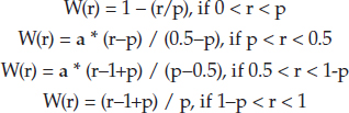
Typically, r= P₀₀, P₀₁, P₁₀, or P₁₁. The W function has the following properties:

• It is minimum and equal to 0 when r = p or r = 1–p, that is, when r does not provide any information about fraud/non-fraud.
• It is maximum and equal to 1 when r=1 or r=0, that is, when you have perfect discrimination between fraud and non-fraud in a given bin.
• It is symmetric: W(r) = W(1–r) for 0 < r < 1. So if you swap Good and Bad (G and B), it still provides the same predictive power.

Now define the predictive power:

The function H is the predictive power for the feature subset {A, B}, having four bins, 00, 01, 10, and 11, corresponding to (A=0, B=0), (A=0, B=1), (A=1, B=0), and (A=1, B=1). Although H appears to be remotely related to entropy, H was designed to satisfy nice properties and to be parameter-driven, because of a. Unlike entropy, H is not based on physical concepts or models; it is actually a synthetic (though useful) metric.

Note that the weights P₀₀… P₁₁ in H guarantee that bins with low frequency (that is, a low-triggering rate) have low impact on H. Indeed, I recommend setting W(r) to 0 for any bin that has less than 20 observations. For instance, the triggering rate for bin 00 is (n₁ + n₅) / (n₁ + … + n₈), observations count is n₁ + n₅, and r = P₀₀ = n₅ / (n₁ + n₅) for this bin. If n₁ + n₅ = 0, set P₀₀ to 0 and W(P₀₀) to 0. I actually recommend doing this not just if n₁ + n₅ = 0 but also whenever n₁ + n₅ < 20, especially if p is low. (If p is very low, say, p < 0.01, you need to over-sample bad transactions when building your training set and weight the counts accordingly.) Of course, the same rule applies to P₀₁, P₁₀, and P₁₁. Note that you should avoid feature subsets that have a large proportion of observations spread across a large number of almost empty bins, as well as feature subsets that produce a large number of empty bins. Observations outside the training set are likely to belong to an empty or almost empty bin and lead to high-variance predictions. To avoid this drawback, stick to binary features, select up to 20 features, and use the (hybrid) hidden decision tree methodology for scoring transactions. Finally, P_ij is the naive estimator of the probability P(A=i, B=j) for i,j = 0,1.

The predictive power H has interesting properties:

• It is always between 0 and 1, equal to 0 if the feature subset has no predictive power and equal to 1 if the feature subset has maximum predictive power.
• A generic version of H (not depending on p) can be created by setting p=0.5. Then the W functions are not shaped like a W anymore; they are shaped like a V.

Data Structure and Computations

You can pre-compute all the bin counts n_i for the top 20 features (that is, features with highest predictive power) and store them in a small hash table with at most 2 × 2²⁰ entries (approximately 2 million; the factor is 2 because you need two measurements per bin: number of Bs, and number of Gs). An entry in this hash table would look like this:

meaning that Bin # 01101001010110100100 has 56 good (G) observations.

The hash table is produced by parsing your training set one time, sequentially: for each observation, compute the flag vector (which rules are triggered, that is, the 01101001010110100100 vector in this example), check if it's good or bad, and update (increase count by 1) the associated hash table entry accordingly, with the following instruction:

Then, whenever you need to measure the predictive power of a subset of these 20 features, you don't need to parse your big data set again (potentially billions of observations), but instead, just access this small hash table. This table contains all you need to build your flag vectors and compute scores for any combination of features that is a subset of the top 20.

You can even do better than top 20, maybe top 30. Although this would create a hash table with 2 billion entries, most of these entries would correspond to empty bins and thus would not be in the hash table. Your hash table might contain only 200,000,000 entries, maybe too big to fit in memory, and requiring a MapReduce/Hadoop implementation.

Even better: build this hash table for the top 40 features. Then it will fully solve your feature selection problem described earlier. However, now your hash table could have up to 2 trillion entries. But if your data set has only 100 billion observations, then, of course, your hash table cannot have more than 100 billion entries. In this case, I suggest that you create a training set with 20 million observations so that your hash table will have at most 20 million entries (probably less than 10 million with all the empty bins) and thus can fit in memory.

You can compute the predictive power of a large number (say, 100) of feature subsets by parsing the big 40-feature input hash table obtained in the previous step. Then for each flag vector and G/B entry in the input hash table, loop over the 100 target feature subsets to update counts (all the n_i) for these 100 feature subsets. These counts are stored/updated in an output hash table. The key in the output hash table has two components: feature ID and flag vector. You then loop over the output hash table to compute the predictive power for each feature subset. This step can be further optimized.

Association Rules to Detect Collusion and Botnets

An example of collusion is when multiple affiliates (or sub-publishers) are associated in the same fraud scheme and share the same resources. Typically, this a Botnet, that is, a set of computer IP addresses infected with a virus that automatically clicks once a day (at most) from each infected machine.

Association rules are fraud detection rules that try to correlate two fraudsters via an external metric. For instance, when an affiliate A is identified as fraudulent, you look at all the IP addresses attached to it. If 50 percent or more of these IP addresses also appear exclusively in association with another affiliate B (and nowhere else), then chances are that B is also part of the fraudulent scheme. Even better: now you look at all the IP addresses attached to B, and you discover that another affiliate, say C, shares 10 percent of them exclusively. Now you've found yet another participant in the fraud scheme. I have successfully identified several additional sources of fraud associated with one fraudster using this technique.

Another rule falling in the same category is the proportion of short visits (less than 20 seconds) that involve two clicks associated with two little, unknown affiliates or referral domains. When this proportion is above some threshold (say, 20 percent of all visits for a specific affiliate), you are likely dealing with fraud. By creating the list of all affiliates found in these two-click visits and then looking at other visits that also involve these affiliates as well as other affiliates, you can detect a larger proportion of bad affiliates.

Finally, Botnets used in click fraud are typically involved in other criminal activities as well and controlled by one operator. So detecting these Botnets with a click fraud detection algorithm can also help detect other crimes: spam, phishing, ID theft, and so on.

Extreme Value Theory for Pattern Detection

Because criminals don't put too much effort into creating artificial traffic that looks, from a statistical point of view, similar to natural traffic, their traffic is full of extreme events that make detection easier. These event probabilities can be estimated (in natural traffic) via Monte Carlo simulations. When discovering an event (in suspicious traffic) with a probability of occurrence below one chance in 1 million, it is a red flag. Of course, if you are tracking billions of events, you will have false positives. Read the section on the curse of big data (Chapter 2) to see how to address this issue. Rare events that were successfully used to detect fraud include:

• Visits with a consistent, perfect 50.00 percent conversion rate, day after day, from the same referral
• A spike in the number of IP addresses that generate exactly eight clicks per day, day after day. (When you plot the distribution of clicks per IP for a specific affiliate or keyword, you see a spike for the value 8.)
• IP addresses with 3+ days of activity per week, with little traffic each day (one or two clicks at most). If you have an affiliate with 40 percent of IP addresses having this pattern, this is an extremely rare event (for most websites) and a red flag.
• A large portion of your traffic (say, 5 percent) has the exact same click score when using your scoring algorithm. This is suspicious.
• Specific keywords found on the web page where the click is taking place: “Viagra,” or some JavaScript tags mostly found on fraudulent websites—or even an empty page!
• Domain name patterns, such as an affiliate using dozens of domains, the vast majority with names such as xxx-and-yyy.com (for instance, chocolate-and-car.com).

All these rules have been successfully used to detect fraud. Multiple rules must be triggered before confirming fraud. For instance, in one case, the bad affiliate simultaneously had the domain name pattern, the identical scores pattern, and the empty web page pattern. It was first discovered because all its clicks had the same score. And by further analyzing the data, I discovered and created the two other rules: domain pattern and empty page pattern.

Digital Analytics

The borderline between data science and other domains, in particular business intelligence (what business analysts do), is not clear. In smaller companies, startups, and non-traditional companies (which hire a significant share of data scientists), several of the project types discussed in this section are handled by one person — the data scientist — who also plays a part-time role as business analyst. Being polyvalent allows you to command higher salaries and experience increased job security.

Domain expertise is critical to succeed in data analytics. A lot of domain expertise is shared with you here, with a focus on rules of thumb and principles that stay valid over time (such as solid SEO principles, e-mail campaign optimization, ad matching, and so on), even though the digital/ad tech industry is constantly changing.

Some of the techniques discussed in this section are typically implemented by vendors (Comscore, Rocket Fuel, and others), search engines (such as Bing, Google, Yahoo), ad networks such as AdKnowledge, or savvy publishers, rather than by advertisers themselves. Advertisers rely on vendors, though large advertisers such as eBay or Cars.com also develop and integrate their own proprietary tools on top of vendor tools. It is important for you to learn about the type of data science work (digital analytics) done by vendors and search engines, because collectively they hire more data scientists than all advertisers combined.

Online Advertising: Formula for Reach and Frequency

How do you effectively compute the reach and frequency of ads for advertisers? The formula discussed here computes reach and frequency for online advertisers to help them determine how many impressions they must purchase to achieve their goals. It is provided to illustrate that sometimes, it is easier to spend two hours to reinvent the wheel, solve the problem mathematically, and get an efficient solution than to spend hours trying to find the solution in the literature or blindly run expensive simulations or computations the way computer scientists traditionally do.

How many ad impressions should an advertiser purchase to achieve a specified reach on a website? I have investigated the problem and found a simple mathematical solution:

Reach = Unique Users − SUM{ U_k ^* ( 1 − P )^k}

The sum is over all positive integers k = 1, 2, and so on. U_k is the number of users turning exactly k pages in the given time period. So you need to compute the distribution of page views per unique user during the targeted time period to compute U_k. P is the ratio of purchased impressions by total pages.

The number of unique users who see the ad n times during the time period in question is given by:

SUM{ U_k ^* C(k, n) ^* Pⁿ ( 1 − P )^k-n}

The sum is over all positive integers k greater or equal to n. C(k, n) = k! / [ n! (k–n)! ] are the binomial coefficients.

In this context, “unique user” represents a user that is counted as one user regardless of the number of visits during the time period in question. A user is a human being, thus robots (web crawlers) should be filters. The IAB (Internet Advertising Bureau) provides definitions, directives, and best practices on how to measure unique users and filter robots. Users are typically tracked via cookies. In the past, many counting methods resulted in a single user being counted multiple times, thus the term “unique user” was created to distinguish users from visits. (Defining concepts such as “unique user” is also part of the data scientist's job.)

E-Mail Marketing: Boosting Performance by 300 Percent

We improved our own open rates on Data Science Central by 300 percent and dramatically improved total clicks and click-through rates using the following strategies, based on data analysis:

• Remove subscribers who did not open the newsletter during the last eight deployments. This produced a spectacular increase in the open rate and also significantly improved our “spam score,” because the newsletter's chances of ending up in a spam box or a spam trap is reduced to almost 0.
• Segment of the subscriber base to better target members, for instance to send a UK conference announcement to members located in Europe, but not to members in Asia or America.
• Detect and stop sending messages that produce low open rates.
• Capture member information (profession, experience, industry, location, and so on) on sign-up to create better segments.
• Grow your subscriber list by:
  • Offering great products for free to subscribers only, for instance e-books, requesting that visitors subscribe to your newsletter if they want to download the book.
  • Requesting that new LinkedIn group members become a member of your community. (The IEEE organization is using the same strategy.)
• A/B testing in real time when deploying an e-mail blast: try three different subject lines with 3,000 subscribers, and then use the subject line with highest click-through rate for the remaining subscribers.
• Identify patterns in subject lines that work well:
  • Research reports from well-respected companies
  • Case studies, success stories
  • Announcement about 10 great articles recently published in top news outlets
  • Salary surveys, job ads from great companies, data science programs from top universities
  • Not using the same great keywords over and over because it kills efficiency. (Poor subject titles that change each time work better than great subject titles that are overused.)

As a result, our mailing list management vendor informed us that our open rate is far above average — and they manage 60,000 clients from small to multimillion e-mail lists!

Optimize Keyword Advertising Campaigns in 7 Days

SEO (search engine optimization) and SEM (search engine marketing) companies regularly hire data scientists, so you need to have a good grasp of how to implement solid, general SEM principles. Here's an example application that is based on careful analysis of keyword performance on Google Analytics:

1. Identify 10 top, high-volume, well-targeted keywords for your business. These are your seed keywords.
2. Create large lists of bid keywords: use Google tools to identify “related keywords” that are related to your seed keywords.
3. Grow further by finding keywords that are related to the keywords obtained in the previous step.
4. Use Google AdWords tools to find keywords that are on your web page, and most important, on your competitors' web pages, choosing the website selection under Find Keywords under Add Keywords when you manage your ad group. Only pick keywords that have a moderate to high volume, and skip keywords with high competition. (Competition and volume statistics are provided by Google on the same page.)
5. Create a campaign, and then add one ad group for all these 2,000 or so keywords. Select your target market (for example, North America + Europe and Google Search + Partners Search) in your campaign settings. Set a max bid that is three or four times higher than what you want.
6. Create four or five different ads so that at least one of them will have a great CTR and will boost click volume.
7. After 4 hours, check your traffic report and pause all keywords with a CTR < 0.20 percent and impression count > 400. This will boost your CTR, further improve your campaigns, and eventually improve your ROI. Then, reduce your max bid by 10 percent because you are probably burning your budget too quickly.
8. On day #2: Check the stats again: Remove low CTR keywords, and reduce the max bid by 10 percent.
9. On day #3: Check the stats again: Remove low CTR keywords, and reduce the max bid by 10 percent. Then isolate keywords with high volume and good CTR, and put them in a separate campaign or ad group. If you are still burning your daily budget too fast, improve targeting by excluding some country and excluding display advertising or other sources of lower traffic quality.
10. On day #4 to #7: Proceed as for day #3, but be less aggressive in your efforts to reduce your max bid: if your CPC goes down too much too quickly, your campaign will collapse.
11. By day #8, you should have several ad groups, each with maybe 50 keywords, which are stable and great for your website, plus a huge ad group (the leftovers of day #1 to #7) that will continue to work as well, requiring occasional monitoring.

Automated News Feed Optimization

Here is another application where data science can help. Each year, billions of dollars are poured into online advertising programs (display and pay-per-click advertising) in an effort to attract visitors to websites. Those websites that attract a high volume of visitors do so because they have great content.

Producing great content can be time-consuming and expensive, so nearly every website publisher wants to automate their content production. In addition, displaying the right content to the right user at the right time dramatically increases ad revenue. Analytic techniques can be used to achieve the goal of relevant and highly targeted content.

For example, at Data Science Central we have achieved the first steps of automated content creation. Our news feed system harvests news from keyword-targeted Google news, selected Twitters and blogs, and also content that we create. Our news feed aggregator was created without writing a single line of code, instead using various widgets, Twitter feeds, and Feedburner. Our analytics news shows up on AnalyticBridge, LinkedIn, and many other places, and is updated in real time to drive good traffic to our websites.

Bigger companies are hiring analytic professionals to optimize these processes. For website publishers and anyone generating online advertising revenue, content is king. My first experiments have proved that optimizing content and news has a bigger impact than optimizing advertising campaigns in terms of increasing advertising revenue. The increased revenue comes from two sources:

• More traffic and more returning users, thus more page views and more conversions.
• Most important is more relevant traffic and higher quality traffic with higher conversion rates, in the attempt to produce news and content that will attract and retain users that also share an interest in the advertisers' products and services.

The fact that Data Science Central is a social network does not play a major role in this dynamic (assuming that spam control has been taken care of effectively). What is critical is content quality and dynamic content, thus our focus on real time news and on including (in our feeds) micro-blogs from a number of small, well-respected data scientists. With strategies such as these, you can turn a social network into a profitable website with growing revenue.

Competitive Intelligence with Bit.ly

Competitive intelligence is part of business intelligence, and is a sub-domain of market research. Bit.ly allows you to check the popularity of web pages published by you or your competitors. It also allows you to see how much traffic you contribute to a web page (one that's your own or some external web page that you promote as part of a marketing campaign), versus how much traffic other people or your competitors generate for the same web page.

Bit.ly, a URL shortener (like tinyurl.com), is the standard tool used in LinkedIn e-mail blasts to shorten long URLs with several tags. (The reason is that LinkedIn blasts are text-only.) Yet, bit.ly offers much more than redirect services; it also has interesting reporting capabilities.

This reporting capability is an example of an excellent big data application, provided you are aware of its simple yet incredibly powerful dashboard. It is also a classic example of big data that is useless unless you are aware of the features coming with it and how to leverage it.

Here a useful example. Consider Figure 6-2, which shows a screenshot of a bit.ly dashboard:

You can find the amount of traffic (page views) from your bit.ly redirects in the “Clicks via Your Shortlink” column. Keep in mind that the same link might have been shortened by other people. That's why there is an extra column labeled “Total Clicks” that tells you the total traffic coming to the target URL, both from you and from other people who used bit.ly to shorten the same URL.

Assess Traffic from the Competition

Assessing traffic from the competition is useful for website publishers or media companies. For the goPivotal link created at 5:15 p.m. (Figure 6-2), 155 clicks are from me and another 114 are from competitors. So I delivered better than competitors on this one. Of course, not everyone uses bit.ly in their marketing campaigns, but many do because it offers traffic statistics by referrer, country, and day to the client. Simply add a + sign at the shortened URL https://bit.ly/11xTDUD+.

Note that the goPivotal link created at 7:22 p.m. contains special proprietary tags and is thus tracked separately. (The bit.ly URL is different, although it points to the same page.) That's why it has 0 clicks attributable to third parties.

Assess Traffic from People Who Shared Your Link

Still continuing with Figure 6-2, the link for “Three classes of metrics” is internal to Data Science Central, so I know that the extra 53 clicks (53 = 155–102) are from people who shared the article with others using bit.ly. If you click “Three Classes of Metrics” on the bit.ly dashboard, then you know who shared the link and how much traffic they generated (in this case, 53 clicks). This information allows you to track who contributes solid traffic to your website.

RealTime bit.ly

RealTime bit.ly is still a beta project (you can access it at http://rt.ly/), but if you use the real-time feature it allows you to fine-tune e-mail campaigns in real time, via A/B testing. For example, if you want to send an e-mail to 100,000 subscribers, you would:

1. Send version A to 2,500 contacts and B to another 2,500 contacts, randomly selected.
2. Wait 10 minutes (even less if possible); see which one performs better (say it's B).
3. Deploy the whole campaign to the remaining 95,000 contacts, using version B of your message.

For instance, the difference between A and B is the subject line, and the success metric is the open rate or click-out rate. For instance, in A, subject line = “Weekly Digest - April 22” and in B, subject line = “Best articles from DSC.” Note that usually when doing e-mail campaign optimization, you are not interested in optimizing just one campaign, but actually all your campaigns. If you want to optimize one campaign, subject line B would win. For global, long-term optimization, A will win.

Measuring Return on Twitter Hashtags

Building a great list of Twitter followers and judiciously using #hashtags seems to be the Holy Grail to grow traffic and reap rewards from social media. A good reference on the subject is the Mashable article “How to Get the Most Out of Twitter #Hashtags” which can be accessed at http://mashable.com/2009/05/17/twitter-hashtags/.

The reality is very different. First, when did you read a Tweet for the last time? Probably long ago. Also, hashtags tend to discourage people from clicking your link. In practice, even with 6,000 real followers, a Tweet will generate 0 clicks at worst and 20 clicks at best. This is true if you count only clicks coming straight from your Tweet and ignore indirect traffic and the multiplier effect described next.

Here's an example of a Tweet with two hashtags, in case you've never seen one before:

Is It Really That Bad?

No, it actually works. First, if your Tweet gets re-Tweeted, it is not difficult to generate tons of additional clicks that can be attributed to Twitter (and even more from other sources), even for subjects as specialized as data science. The Twitter multiplier can be as high as 3.

For instance, a great article published in our Data Science Central weekly digest gets 800 clicks that are directly attributed to the eBlast sent to more than 60,000. After 12 months, the article has been viewed 12,000 times. When you analyze the data, you find that 2,400 of the total visits can be attributed to Twitter (people reposting your link and sharing it via Twitter).

There are also some other positive side effects. Some publishers run web crawlers to discover, fetch, and categorize information, and #hashtags are one of the tools they use to detect and classify pieces of news. Data Science Central is one of them—both as a crawler and as a crawlee. The same publishers also publish lists of top data scientists. Their lists are based on who is popular on specific hashtags regardless of whether the Tweets in questions are generated automatically (syndicated content) or by a human being.

And while a Tweet full of special characters is a deterrent for the average Internet user, it is much less so for geeks. (If you read this book, chances are that you are, at least marginally, a geek.) However, you must still comply with the following rules:

• You don't have more than two hashtags per Tweet.
• The hashtags are relevant.
• 50 percent of your Tweets have no hashtags.

Otherwise, people will stop reading what you post and then you are faced with the challenge of finding new followers faster than you are losing old ones.

Hashtags are particularly suited to comment on a webinar as it goes live: INFORMS could use the #INFORMS2013 hashtag for people commenting on their yearly conference. Hashtags are also helpful to promote or discuss some event. For instance, we created #abdsc to reward bloggers Tweeting about us.

Still, it is not so easy to be listed under Top rather than All People on Twitter when posting a Tweet. And if you are not in the Top list, your hashtag has no value. In addition, you can be a victim of hashtag hijacking: hashtag spammers abusing a popular hashtag to promote their own stuff.

Figure 6-3 is based on recent posts at Data Science Central tracked via bit.ly and shows that a blog post can easily see its traffic statistics triple (rightmost column), thanks to other people who like what you wrote and re-Tweet or re-post it on their blogs. Note that the fewer internal clicks, the bigger the multiplier: when we don't do much to promote one of our posts, then other bloggers promote it on our behalf. The most extreme case here is one internal click with multiplier 53.

Will Hashtags Work for You?

An easy way to check whether hashtags provide a lift is to perform some A/B testing. You can use the following protocol:

1. Over a 14-day time period, Tweet two links each day: one at noon and one at 6 p.m.
2. The first day, in the morning, add the hashtag #datascience to your Tweet. Don't add a hashtag in the evening.
3. On the second day, do the reverse: no hashtag at noon, but add a hashtag #datascience at 6 p.m.
4. Keep alternating noon and 6 p.m. to determine when to add the hashtag.
5. Attach a specific query string to each link, for instance, ?date=0528&hashtag=yes&time=6pm to the URL you are Tweeting (before shortening the URL). This is for tracking purposes.
6. Use bit.ly to shorten your URLs.

For example, your Tweet (hashtag version) could be something like this:

Note that when you click https://bit.ly/11wpSXi, the query string shows up in the reconstructed URL in your browser (after the redirect). What's more, you can monitor how many clicks you get by looking at https://bit.ly/11wpSXi+ (same bit.ly URL, with + added at the end).

After 20 days, you can now perform a statistical analysis to check the following:

• Hashtags boost the number of direct clicks.
• Hashtags boost the multiplier effect discussed earlier.

You can detect if click variations are explained by time, weekend/weekday, or some other factor such as link and whether hashtags positively contribute, and quantify this contribution.

Real-Time Detection of Viral Tweets

Micro-memes are emergent topics for which a hashtag is created, used widely for a few days, and then disappears. How can they be detected and leveraged? Journalists and publishers are particularly interested in this.

TrendSpottr and Top-Hashtags are websites offering this type of service. However, they rely on sample data—a major drawback to discover new, rare events that suddenly spike. It is especially difficult because these memes use made-up keywords that never existed before, such as #abdsc or #hashtagABtest.

Also, Top-Hashtag worked with Instagram, but not with Twitter, last time I checked. Hashtags also work on Google+. For data science, the most interesting large social networks are LinkedIn (more professional), Google+, Quora (more geeky), and Twitter. So identifying in real time new trends that are emerging on these networks is important.

One solution consists of following the most influential people in your domain and getting alerts each time one of their new hashtags get 10+ Tweets. If some new hashtag from an unknown person starts creating a lot of buzz, these influencers (at least some of them) will quickly notice, and you will, too, because you follow the influencers. Just pick up the right list of keywords and hashtags to identify top influencers: data science, Hadoop, big data, business analytics, visualization, predictive modeling, and so on. Some lists of top influencers are publicly available.

The key message of this discussion is twofold: currently, good algorithms to detect signal from noise and categorize Tweets are yet to be developed, and they involve data science and NLP (natural language processing). Such algorithms are particularly useful to website publishers, content managers, and journalists.

Improving Google Search with Three Fixes

These big data problems probably impact many search engines, which is one piece of evidence that there is still room for new startups to invent superior search engines. Data scientists are well equipped to identify these problems and quantitatively measure whether they are big or small issues, to help prioritize them. These problems can be fixed with improved analytics and data science. Here are the problems and the solutions.

Outdated Search Results

Google does not do a good job of showing new or recently updated web pages. Of course, new does not mean better, and the Google algorithm favors old pages with a good ranking, on purpose—maybe because the ranking for new pages is less reliable or has less history. (That's why I created statistical scores to rank web pages with no history.) To solve this problem, the user can add 2013 to Google searches. And Google could do that, too, by default. For instance, compare search results for the query data science with those for data science 2013. Which one do you like best? Better, Google should allow you to choose between “recent” versus “permanent” search results when you do a search.

The issue here is to correctly date web pages, which is a difficult problem because webmasters can use fake timestamps to fool Google. But because Google indexes most pages every couple of days, it's easy to create a Google timestamp and keep two dates for each (static) web page: date when first indexed and date when last modified. You also need to keep a 128-bit signature (in addition to related keywords) for each web page to easily detect when it is modified. The problem is more difficult for web pages created on the fly.

Wrongly Attributed Articles

You write an article on your blog. It then gets picked up by another media outlet, say The New York Times. Google displays The New York Times version at the top and sometimes does not even display the original version at all, even if the search query is the title of the articles, using an exact match. You might argue that The New York Times is more trustworthy than your little unknown blog or that your blog has a poor page rank. But this has two implications:

It creates a poor user experience. To the Google user, the Internet appears much smaller than it actually is.

Webmasters can use unfair strategies to defeat Google: using smart Botnet technology with the right keyword mix to manufacture tons of organic Google queries, but manufacture few clicks—only on their own links. This will lower the organic CTR for competitors but boost yours. It is expected that this “attack” would fix your content attribution problem.

Another, meaner version of the CTR attack consists of hitting the culprit website with lots of organic Google clicks (Google redirects) but no Google impression. This could fool Google algorithms into believing that the website in question is engaging in CTR fraud by manipulating click-in ratios, and thus get them dropped from Google. At the same time it will create a terrible impression-to-conversion (click-out) ratio for advertisers showing up on the incriminated landing pages, hitting display ads particularly hard, causing advertisers to drop the publisher. In short, this strategy could automatically take care of copyright infringement using two different levers at once: click in and click out. It must be applied to one violator at a time (to avoid detection) until they are all gone. If properly executed, nobody will ever know who did the attack; maybe nobody will ever find out that an attack took place.

One easy way for Google to fix the problem is, again, to correctly identify the first version of an article, as described in the previous paragraph.

Favoring Irrelevant Web Pages

Google generates a number of search result impressions per week for every website, and this number is extremely stable. It is probably based on the number of pages, keywords, and popularity (page rank) of the website in question, as well as a bunch of other metrics (time to load, proportion of original content, niche versus generic website, and so on). If every week Google shows exactly 10,000 impressions for your website, which page or keyword match should Google favor?

Google should favor pages with low bounce rate. In practice, it does the exact opposite.

Why? Maybe if a user does not find your website interesting, he performs more Google searches and the chance of him clicking a paid Google ad increases. So bad (landing page) user experience financially rewards Google.

How do you fix it? If most users spend little time on a web page (and Google can easily measure time spent), that web page (or better, that web page or keyword combination) should be penalized in the Google index to show up less frequently. Many publishers also use Google Analytics, which provides Google with additional valuable information about bounce rate and user interest at the page level.

However, you might argue that if bounce rate is high, maybe the user found the answer to his question right away by visiting your landing page, and thus the user experience is actually great. I disagree, since at Data Science Central, each page displays links to similar articles and typically results in subsequent page views. Indeed, the worst bounce rate is associated with Google organic searches. More problematic is the fact that the bounce rate from Google organic is getting worse (while it's getting better for all other traffic sources), as if the Google algorithm lacks machine learning capabilities or is doing a poor job with new pages added daily. In the future, longer articles broken down into two or three pages will hopefully improve the bounce rate from Google organic (and from other sources as well).

Improving Relevancy Algorithms

Here you focus on ad relevancy in the context of online advertising such as search engine advertising. When you see ads on search result pages or elsewhere, the ads that display in front of your eyes (should) have been highly selected to maximize the chance that you convert and generate ad revenue for the publisher or search engine.

If you think you see irrelevant ads, either they are priced cheaply or Google's ad relevancy algorithm is not working well. Sometimes it's due to cheap ads, sometimes poor scoring, and you could argue that sometimes it's because the advertiser is doing a poor job of keyword selection and targeting.

Ad scoring algorithms used to be simple, the score being a function of the max bid paid by the advertiser and the conversion rate CTR. This led to abuses: an advertiser could generate bogus impressions to dilute competitor CTR, or clicks on its own ads to boost its own CTR, or a combination of both, typically using proxies or Botnets to hide the scheme, thus gaining unfair competitive advantage over search engines. Note that search engines use traffic quality scores. Indeed, I have been hired in the past, as a data scientist, to reverse engineer some of these traffic quality algorithms, as well as perform stress tests to see what makes them fail.

Recently, in addition to CTR and max bid, ad networks have added ad relevancy to their ad scoring mix (that is, in the algorithm used to determine which ads you will see, and in which order). In short, ad networks don't want to display ads that will make the user frustrated — it's all about improving user experience and reducing churn to boost long-term profits. How Does Ad Relevancy Scoring Work?

There are three components in the mix:

• The user visiting a web page hosting the ad in question
• The web page where the ad is hosted
• The ad itself, that is, its text or visual content, or other metrics such as size, and so on

The fourth important component—the landing page—is not considered in this short discussion. (Good publishers scrape advertiser landing pages to check the match between a text ad and its landing page, and eliminate bad adware.)

The Solution

You will need to create three taxonomies:

• Taxonomy A to categorize returning users based on their interests, member profile, or web searching history
• Taxonomy B to categorize web pages that are hosting ads, based on content or publisher-provided keyword tags
• Taxonomy C to categorize ads, based on text ad content, or advertiser-provided keywords to describe the ad (such as bid keyword in PPC campaigns, or ad title)

The two important taxonomies are B and C, unless the ad is displayed on a generic web page, in which case A is more important than B. So ignore taxonomy A for now. The goal is to match a category from Taxonomy B with one from Taxonomy C. Taxonomies may or may not have the same categories, so in general it will be a fuzzy match where, for instance, the page hosting the ad is attached to the categories Finance/Stock Market in Taxonomy B, while the ad is attached to the categories Investing/Finance in Taxonomy C. So you need to have a system in place to measure distances between categories belonging to two different taxonomies.

How to Build a Taxonomy

There are a lot of vendors and open source solutions available on the market, but if you want to build your own taxonomies from scratch, here's one way to do it:

1. Scrape the web (DMOZ directory with millions of precategorized web pages that you can download freely is a good starting point), extract pieces of text that are found on the same web page, and create a distance to measure proximity between pieces of text.
2. Clean and stem your keyword data.
3. Leverage your search query log data: two queries found in the same session are closer to each other (with respect to the preceding distance) than arbitrary queries
4. Create a table with all pairs of “pieces of text” that you have extracted and that are associated (for example, found on the same web page or same user session). You will be OK if your table has 100 million such pairs.

Say that (X, Y) is such a pair. Compute n1 = # of occurrences of X in your table, n2 = # of occurrences of Y in your table, and n12 = # of occurrences where X and Y are associated (for example, found on the same web page). A metric that tells you how close X and Y are to each other would be R = n12 / SQRT(n1 x n2). With this dissimilarity metric (used for instance at http://www.frenchlane.com/kw8.html) you can cluster keywords via hierarchical clustering and eventually build a taxonomy—which is nothing more than an unsupervised clustering of the keyword universe with labels manually assigned to (say) the top 20 clusters, with each representing a category.

Ad Rotation Problem

When an advertiser uses (say) five versions of an ad for the same landing page and the same AdWords keyword group (keywords purchased on Google), how frequently should each of the five ads show up? From Google's perspective, the optimum is achieved by the ad providing the highest revenue per impression, whether the advertiser is charged by impression (CPM model) or by the click (pay-per-click). For the advertiser, the ad commanding the lowest cost-per-click (CPC) is sometimes the optimum one, although it might generate too few clicks.

However, Google cannot just simply show 100 percent of the time the ad with the highest revenue per impression. This metric varies over time, and in 2 weeks the optimum ad could change, as users get bored seeing the same ad all the time or new keywords are purchased. So Google will show the five ads, semi-randomly. The optimum ad is displayed much more frequently, and the worst one very rarely.

But how do you define “much more frequently” and “very rarely”? Of course, it depends on the impression-to-click ratio multiplied by the CPC. Interestingly, it seems that Google has chosen a logarithm relationship between how frequently an ad is displayed and its CTR (impression-to-click ratio). The CPC is ignored in Google's model, at least in this example.

What do you think about Google's choice of a logarithmic distribution? Is it:

• Arbitrary?
• Coincidental? (More tests would show that the relation found is wrong and just happened by chance for this specific ad campaign.)
• The result of deep investigations by Google data scientists?

And why is the CPC decoupled? Maybe to avoid fraud and manipulations by advertisers.

If you check the figures at http://www.analyticbridge.com/group/webanalytics/forum/topics/ad-serving-optimization you'll see that the optimum ad is served 76.29 percent of the time, and the second best one only 10.36 percent of the time, despite both having a similar CTR and a similar CPC. The CPC is not taken into account, just the CTR; models involving CTR have a worse R^2 (goodness of fit). Models other than logarithmic have a worst R^2 than logarithmic.

Miscellaneous

This section discusses a few data science applications in various other contexts. These applications are routinely encountered in today's markets.

Better Sales Forecasts with Simpler Models

A common challenge is how to make more accurate sales forecasts. The solution is to leverage external data and simplify your predictive model. In 2000, I was working with GE's analytic team to improve sales forecasts for NBC Internet, a web portal owned by NBC. The sales/finance people were using a basic formula to predict next month sales based mostly on sales from the previous month. With GE, I started to develop more sophisticated models that included time series techniques (ARMA—auto regressive models) and seasonality but still were entirely based on internal sales data.

Today, many companies still fail to use the correct methodology to get accurate sales forecasts. This is especially true for companies in growing or declining industries, or when volatility is high due to macroeconomic, structural factors. Indeed, the GE move toward using more complex models was the wrong move: it did provide a small lift but failed to generate the huge lift that could be expected switching to the right methodology.

The Right Methodology

Most companies with more than 200 employees use independent silos to store and exploit data. Data from the finance, advertising/marketing, and operation/inventory management/product departments are more or less independent and rarely merged together to increase ROI. Worse, external data sources are totally ignored.

Even each department has its own silos: within the BI department, data regarding paid search, organic search, and other advertising (print, TV, and so on) are treated separately by data analysts that don't talk to each other. Although lift metrics from paid search (managed by SEM people), organic search (managed by SEO people), and other advertising are clearly highly dependent from a business point of view, interaction is ignored and the different channels are independently—rather than jointly—optimized.

If a sale results from a TV ad seen 3 months ago, together with a Google ad seen twice last month, and also thanks to good SEO and landing page optimization, it will be impossible to accurately attribute the dollar amount to the various managers involved in making the sale happens. Worse, sales forecasts suffer from not using external data and econometric models.

For a startup (or an old company launching a new product), it is also important to accurately assess sales growth using auto-regressive time series models that take into account advertising spend and a decay function of time. In the NBC Internet example, TV ads were found to have an impact for about 6 months, and a simple but good model would be:

where the time unit is 1 month (28 days is indeed better), and both g and f are functions that need to be identified via cross-validation and model fitting techniques (the f function corresponding to the ARMA model previously mentioned).

Following is a list of factors influencing sales:

• Pricing optimization (including an elementary price elasticity component in the sales forecasting model), client feedback, new product launch, and churn should be part of any basic sales forecasts.
• Sales forecasts should integrate external data, in particular:
  • Market share trends: Is your company losing or gaining market share?
  • Industry forecasts (growth or decline in your industry)
  • Total sales volume for your industry based on competitor data. (The data in question can easily be purchased from companies selling competitive intelligence.)
  • Prices from your top competitors for same products, in particular, price ratios (yours versus the competition's).
  • Economic forecasts: Some companies sell this type of data, but their statistical models have flaws, and they tend to use outdated data or move very slowly to update their models with fresh data.

A Simple Model

Identify the top four metrics that drive sales among the metrics that I have suggested (do not ignore external data sources—including a sentiment analysis index by product, that is, what your customers write about your products on Twitter), and create a simple regression model. You could get it done with Excel (use the data analysis plug-in or the linest function) and get better forecasts than you would using a more sophisticated model based only on internal data coming from just one of your many data silos.

How to Hire a Good Sales Forecaster

You need to hire some sort of a management consultant with analytic acumen who will interact with all departments in your organization, gather, merge, and analyze all data sources from most of your silos, integrate other external data sources, and communicate with both executives and everybody in your organization who owns or is responsible for a data silo. He will recommend a solution. Conversations should include data quality issues, which metrics you should track moving forward, and how to create a useful dashboard for executives.

Better Detection of Healthcare Fraud

The Washington Education Association (WEA, in Washington State) is partnering with Aon Hewitts (Illinois), a verification company, to eliminate a specific type of health insurance fraud: teachers reporting non-qualifying people as dependents, such as an unemployed friend with no health insurance. The fraud is used by “nice” people (teachers) to provide health insurance to people who would otherwise have none, by reporting them as spouses or kids.

Interestingly, I saw the letter sent to all WEA teachers. It requires them to fill out lots of paperwork and provide multiple identity proofs (tax forms, birth certificates, marriage certificates, and so on) similar to ID documents (I9 form) required to be allowed to work for a company.

It is easy to cheat on the paper documentation that you have to mail to the verification company (for example, by producing fake birth certificates or claiming you don't have one, and so on). In addition, asking people to fill out so much paperwork is a waste of time and natural resources (trees used to produce paper) and results in lots of errors, privacy issues, and ID theft risk, and costs lots of money for WEA.

So why don't they use modern methods to detect fraud: data mining techniques to detect suspicious SSNs, identifying SSNs reported as dependent by multiple households based on IRS tax data, SSNs not showing up in any tax forms submitted to the IRS, address mismatch detection, and so on? (Note that a 5-day-old baby probably has no record in the IRS database, yet he is eligible as a dependent for tax or health insurance purposes.)

Why not use data mining technology, instead of paper, to get all of the advantages that data mining offers over paper? What advantages does paper offer? I don't see any.

Attribution Modeling

I was once asked to perform a study for NBC. It was running advertising using a weekly mix of TV shows at various times to promote its Internet website. I was asked to identify which TV shows worked best to drive new users to the website. Each week, it was using pretty much the same mix of 10 to 12 shows out of 20 different shows. GRT data (number of eyeballs who watched a particular TV show at a particular time) were collected, as well as weekly numbers of new users, over a 6-month time period. No A/B testing was possible, so the problem was quite complicated.

Here's how I solved the problem. I computed a distance for all pairs of weeks {A, B}, based on which TV shows were used in the weeks in question, as well as the total GRT of each week (high GRT results in many new users unless the TV ad is really bad). I then looked at pairs of weeks that were very similar (in terms of GRTs and show mixes) and close in time (no more than 2 months apart). I focused on pairs where week A had one more show, say show S, compared with week B. Week B did not have S but instead had an extra show not shared with A, say show T. Actually, it was a bit more complicated than that. I allowed not just one, but two different shows. But for the sake of simplicity, stick with this example: show S in week A and not in week B, and show T in week B but not in week A. If week A had more new users than B, I would adjust the performance index of shows S and T as follows: P(S) = P(S) + 1, P(T) = P(T) − 1. The converse was done; A had fewer new users than B.

To identify the best performing shows, all that was left to do was to rank shows by their performance indexes. Law & Order was the winner and was used more often in the mix of TV shows used to promote the website.

Forecasting Meteorite Hits

This example can be used for training purposes as part of the curriculum to become a data scientist. This section describes the different steps involved in a typical, real analysis: from understanding the problem (how to forecast meteorite hits) to providing an answer.

Conclusions are based on manual estimates, which make sense in this context. This section also describes how much a consultant would charge for this analysis, disproving the fact that data scientists are expensive.

The conclusions of the statistical analysis are different from what you've read in the press recently: the Russian meteor is an event said to occur once every 40 years, according to journalists.

Following is a statistical analysis in eight steps:

1. Define the scope of analysis. This is a small project to be completed in 10 hours of work or less, billed at $100/hour. Provide the risk of meteorite hit per year per meteorite size.
2. Identify data and caveats. You can find and download the data set at http://osm2.cartodb.com/tables/2320/public#/map.

   Data about identified meteors—those that have not hit Earth yet but occasionally fly by—are not included in this analysis. Identifying and forecasting the number of such meteors would be the scope of another similar project.

3. Data cleaning: the data seem comprehensive, but they are messy. The database seems to take years to get updated (many fewer meteorites in 2000–2010 than one decade earlier). Some years have very little data. The number of meteorites started to explode around 1974, probably the year when collecting data started. Five fields are of special interest: meteorite type, size, year, and whether the date corresponds to “when it fell” or “when it was found.” Another field not considered here is location. Discard data prior to 1900.
4. Exploratory analysis: Some strong patterns emerge, despite the following:
   • Messy data
   • Recent years with missing observations or data glitches
   • Massive meteorites that are both extremely rare and extremely big—creating significant volatility in the number of tons per year
   • The fact that most meteorites are found (rather than being seen falling) with unknown time lags between “discovery” and “fall.” And “found” sometimes means a fragment rather than the whole rock.

   These patterns are:

   • Smaller meteorites are now detected because of the growing surface of inhabited land and better instruments.
   • The frequency of hits decreases exponentially with size (measured in grams in the data set).
   • Grouping by size using a logarithmic scale and grouping by decade makes sense.
5. The actual analysis: you can find the Excel spreadsheet with data and formulas at http://bit.ly/1gaiIMm. It helps to include the “found” category in the analysis (despite its lower accuracy); otherwise, the data set is too small. The data are summarized (grouped by decade and size) on the Analysis tab in the spreadsheet, using a basic Excel function such as Concatenate, Countif, Averageif, log, int.

   There are nine group sizes with at least one observation: from size 0 for the smallest meteorites to size 8 representing a 9 to 66 ton meteorite—like the one that exploded over Russia. According to the data set, no size 8 was found in the last 40 years, and maybe this is why people claim that the 2013 Russian bang occurs every 40 years. But there were five occurrences between 1900 and 1950. Not sure how reliable these old numbers are. Here, the size is computed as INT(0.5 * log m) where m is the mass of the meteorite in grams.

   Also look at size ratios, defined as the number of meteorites of size k divided by the number of meteorites of size k + 1 (for a given decade), to build a predictive model. Analyze how variations occur in these ratios, as well as ratio variations across decades for a fixed size k.

   A quick regression where Y = ratio (1950–2010 aggregated data) and X = size shows a perfect linear fit (R^2 > 0.98), as shown in the top figure at http://www.analyticbridge.com/profiles/blogs/great-statistical-analysis-forecasting-meteorite-hits. In the figure, I have excluded size 0 (it has its own problems), as well as sizes 8 and 7, which are rare (only one occurrence for size 8 during the time period in question). The total number of meteorites across all sizes is 31,690.

   I tried separate regressions (size versus ratio) for each decade to see if a pattern emerges. A pattern does emerge, although it is easier to detect with the brain than with a computer: the slope of the regression decreases over time (very, very roughly and on average), suggesting that more small meteorites have been found recently, whereas the number of large meteorites does not increase much over time (for size 5+).

6. Model selection: two decades show relatively good pattern stability and recency: 2000–2010 and 1990–2000. Likewise, sizes 5 and 4 show pattern stability (growth over time for size 4, rather flat for size 5). I used these two time periods and sizes to build initial forecasts and estimating slopes, eventually providing two predictions for the chance of a hit (lower and upper bound) for any size. The span (or confidence interval) grows exponentially with size, as you would expect.

   The ratios in white font/red background in the spreadsheet represent manual estimates (sometimes overwriting actual data) based on interpolating the most stable patterns. No cross-validation was performed. Much of the validation consisted of identifying islands of stability in the ratio summary table in cells Y1:AG8.

7. Prepare forecasts, as shown in Figure 6-4.

   

   Figure 6-4: Predicting meteorite hits based on size

   A formula to compute yearly occurrences as a function of actual weight can easily be derived:

   Yearly_Occurrences(weight) = 1/(A + B* log(weight))

   Here's an exercise for you: estimate A and B based on Figure 6-4.

   Based on the table, it makes the “every 40 year” claim for the 2013 Russian bang plausible. The Russian meteorite might have exploded louder than expected because of the angle, composition, or velocity. Or maybe the weight of the meteorite is based on the strength of its explosion, rather than the other way around.

   There were no meteorites of sizes 9, 10, 11, or 12 in the data set and few of size 8, so the associated risks (for these sizes) are based on pure interpolation. Yet they constitute the most interesting and valuable part of this study.

8. Followup: A more detailed analysis would involve predictions broken down by meteor type (iron and water), angle, and velocity. Also, the impact of population growth could be assessed in this risk analysis. In this small analysis, it is indeed implicitly factored in. Also, you could do some more conventional cross-validation, maybe making a prediction for 2013, and see how close you are for meteorites of sizes 0 to 4. Discussing this with the client can provide additional work for the consultant and more value for the client.

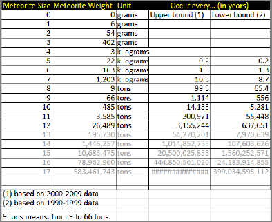
This is a small analysis and there is not a real metric to measure model performance or ROI on this project. Many projects do, just not this one. It is also unusual for a statistician or data scientist to make intelligent guesses and handmade predictions. It is commonplace in engineering, though.

Data Collection at Trailhead Parking Lots

This section illustrates that data science can be used in many different contexts. It also focuses on experimental design and sampling, a domain of statistical science that should be included in data science. Finally, it shows that “no data” does not mean you can't do anything. Data scientists should be able to tell how to first create (in a way that helps data science) and then track data, when the data are initially absent.

Trailhead parking lots are notorious for crime activity. These remote, unpatrolled locations, hidden in dense forests, attract all sorts of bad people. One original crime is thieves stealing the park fees paid by hikers. These fees consist of $5 bills inserted by trail users (hikers) in an envelope and dropped in a locked mailbox at the trailhead. These wooden boxes are easy to break and repair, for the purpose of stealing some of the $5 bills. A smart thief would probably visit 10 trailhead parking lots with lots of hikers once a week, at night, and steal 50 percent of the envelopes. (Stealing 100 percent would attract the police's attention.) It could easily generate a $50,000 income a year, with little work and low risk—especially because there are so many agencies involved in charging and collecting these fees. A smart thief would steal only $5,000 a year from each agency but would target 10 different agencies associated with 10 different popular hikes.

I'm not saying this crime is happening, but it is a possibility. Another type of crime would be perpetrated by official employees collecting these fees and keeping a small percentage for themselves.

How would you detect this crime? Installing webcams might be too expensive in these remote locations with no Internet and no cell phone service. How can you prevent this crime from happening? And how can you make sure every hiker pays the fee—usually $5 per day? Now answer some of these questions.

We asked readers on Data Science Central to answer the question: how can you detect crime and fix it with data science? The answers, which offer real data science solutions, include using experimental design, creating data, tracking numbers on dollar bills or money collected by employees, employee rotation, and others. (If you would like to see more of the answers in more detail, see http://www.analyticbridge.com/profiles/blogs/how-would-you-detect-and-stop-this-type-of-crime in the comments section.)

Other Applications of Data Science

Data science is applied in many other domains and industries. For instance:

• Oil industry: Use statistical models to detect oil fields by drilling as few wells as possible. If you could drill 10 wells, 5 producing oil, 5 not producing oil, and assuming the shape of the oil field is a convex domain, then the problem consisted of estimating the border of the domain (oil field), based on 5 outside and 5 inside points, and then drill wells with a high probability of finding oil.
• Credit scoring: One of the issues preventing new models from being created and deployed is regulations. Larger banks have statisticians that work on credit models for loans and the models must be approved by regulators, the FDIC (see http://1.usa.gov/1aLJ9aa). New methodology pioneered by John Elder, for better scoring, relies on ensemble methods. Note that similar statistical modeling regulations that can kill data science innovation apply to clinical trials.

Data science applications cover most fields: sensor data, mobile data, smart grids (optimizing electrical networks and electricity pricing), econometrics, clinical trials, operations research (optimizing business processes), astronomy, plagiarism and copyright infringement detection, and even computational chemistry (designing new molecules to fight cancer).

Summary

This chapter discussed case studies, real-life applications, and success stories involving data science. It covered various types of initiatives, ranging from stock market techniques to advertising mix optimization, fraud detection, search engine optimization (for search companies), astronomy (forecasting meteorite hits), automated news feed management, data encryption, e-mail marketing, and various relevancy problems (online advertising).

The next chapter focuses on helping you get employed as a data scientist. It includes sample resumes, more than 90 job interview questions, companies that routinely hire data scientists, and typical job titles for data scientists.