Chapter 6: HFT Optimization – Architecture and Operating System

In the previous chapter, we were presented with an outline of how a computer works with a focus on the main components that relate to HFT. In this chapter, we will discuss some of the commonly employed computer science and architecture optimization techniques specifically as they relate to HFT applications. We will provide some context with the details of how certain specific operations work in terms of what goes on under the hood, why they are inefficient, slow, and problematic for HFT software, and what techniques are used to get around it.

Some of the operations and constructs we will discuss are context switching between threads, locks to concurrently access shared data structures, and memory management/optimization motivations and techniques.

HFT is primarily an arms race where each HFT competitor is trying to execute trades as quickly as possible. So, getting to grips with the computer science fundamentals for the topics we cover in this chapter will help the reader understand how to produce extremely optimized and high-performing HFT applications. We will cover the following topics in this chapter:

• Understanding context switches
• Building lock-free data structures
• Pre-fetching and pre-allocating memory

Performance mental model

When we talk about HFT optimizations, we could use an endless number of techniques to reach the lowest possible latency. The most important question to ask is what we are trying to achieve – what level of performance is good enough for HFT trading strategies? In this book, we present a lot of optimizations and it would be overwhelming and time consuming to implement all of them. In order to guide the readers through all the optimizations, we will differentiate optimizations by considering them in terms of three groups that lowers the latency by a specific number of microseconds, represented by the following icons:

• : Lower than 20 microseconds
• : Lower than 5 microseconds
• : Lower than 500 nanoseconds

Let's get started!

Understanding context switches

A context switch in computer science is the operation or set of tasks by which all the states associated with a running process or thread is saved and the state associated with a different process or thread to be run next is restored so that it can resume where the execution left off. The principle of context switching is the cornerstone on which modern Operating Systems' (OSs') support for multitasking is based, and which gives the illusion of running a lot more processes than the number of CPU cores available in the hardware.

Types of context switches

Context switches can be grouped into different types depending on which aspect of the context switching process we look at. We will briefly discuss them as follows.

Hardware or software context switches

Context switches can be performed in hardware or software. In hardware context switching, special hardware features such as Task State Segments (TSSs) can be used to save the register and processor state for the currently running process and then jump to a different process. In software context switches, the current stack pointer is saved and the new stack pointer is loaded to execute the new code. Registers, flags, data segments, and all other relevant registers are also pushed onto the old stack and popped off the new stack.

Hardware context switching requires special registers and/or processor instructions to implement and can be expected to be faster than software context switching due to the availability of special registers and instructions. However, in some cases, hardware context switches can be slower than software context switches since it needs to save all registers. Modern OSs, however, choose to implement context switching in software due to better fault tolerance and the ability to customize what registers are saved and restored.

Context switches between threads or processes

Another way to classify different types of context switching is whether it occurs between threads or processes. The latency associated with context switching between processes is referred to as process switching latency and between threads is referred to as thread switching latency. If threads or processes share the same address space, then the context switching is faster because the code to be executed is most likely already loaded in the cache/memory due to the shared address space. During context switching, not only does the OS need to remove and reload code from the cache and memory; it also has to clean/flush the data structure that holds the memory address mapping known as virtual memory space. So, context switching between threads is generally faster since they share the virtual memory space, and flushing and cleaning/invalidating the Translation Lookaside Buffer (TLB) is not necessary. The details of virtual memory space and the TLB are advanced OS concepts and out of the scope of this book, so we will not dive into too many details on those topics.

Why are context switches good

Context switching is worthwhile functionality for most applications that have a good mixture of user inputs, disk Input/Output (I/O), and CPU-intensive processing, such as the Microsoft Office suite of applications, video games, or browsers. Within the HFT ecosystem, some (but not all) components such as logging processes, Graphical User Interface (GUI) applications, and so on benefit from context switching. As mentioned previously, supporting multitasking in modern OSs would not have been possible without context switching. The most important ones would be multitasking, interrupt handling in the OS, and switching between user and kernel modes (often invoked when handling interrupts). We will discuss them in the following sections.

Multitasking

All modern OSs have a task scheduler that switches out one process for another to be processed in the CPU. There can be several reasons for a running process to be switched out. For example, when the process is completed, or it is stuck on an I/O or synchronization operation – in both cases, waiting for input from another process, thread, or disk. It is possible for a thread or process to be switched out to prevent a single CPU-intensive thread or process from hogging all the CPU resources and preventing other waiting tasks from being finished, which is known as CPU starvation.

Interrupt handling

Interrupt-driven data flow is common in most modern architectures. When processes need to access resources, such as fetching something from or writing something to disk (disk I/O) or sockets/Network Interface Cards (NICs) – the process does not sit around consuming CPU resources waiting for the operations to finish. This is mainly because disk and network I/O operations are orders of magnitude slower than CPU operations, so this would waste a tremendous amount of CPU resources.

In the interrupt-driven architecture, such a process initiates the I/O operation and is blocked on that operation. Then the scheduler context switches out that process and resumes another waiting process. Behind the scenes, the OS also installs an interrupt handler with the hardware, which will interrupt the running process at the time the operation finishes and wake up the process that initiated the request and let it handle the request completion.

User and kernel mode switching

In the previous section, we saw an interrupt-driven example where the disk or packet read finishes and then the interrupt handler wakes up the process that initiated the request. In that sequence of events, part of the operation is carried out in kernel space, namely invoking the interrupt handler with the necessary signals, and the new process acquiring some CPU resources and starting to process the data. The actual data processing usually takes place in user space and depends on the application itself. This is not the only case where there are switches made between kernel and user space; some instructions invoked by a process running in user space also force a transition into kernel mode. For most systems, this switching does not invoke a context switch, but it might happen for some systems when switching between user and kernel mode. In the next section, we will look at the sequence of actions involved in a context switch operation. A good understanding of this is important because it then becomes clear how context switching can become expensive in the context of HFT applications.

Steps and operations involved in a context switch operation

Let's look at some of the operations involved in a context switch – specifically the tasks involved in saving the state of the currently running thread or process and restoring the state of the next thread or process to be run, as decided by the task scheduler. Please note that this section provides a high-level view of tasks involved and might be missing a few specific details for specific architectures; that is, each architecture and OS has caveats specific to them aside from this list, but this list still serves as a generic list of steps involved:

1. Saving the state of the current process involves saving the state in what is often known as a Process Control Block (PCB). That contains the registers, Stack Pointer register (SP), Program Counter (PC), and memory maps. There are also various tables and lists for the current thread or process.
2. There are likely a few steps to flush and/or invalidate the cache and flush the TLB, which handles the virtual memory address to physical memory address translations.
3. Restoring the state for the next thread or process to be run is the opposite step of what it takes to save the state, that is, restoring the registers and data contained in the PCB for the thread or process to be restored.

This section presented a higher-level view of the all the steps involved in facilitating a context switch. In practice, there can be additional steps depending on the hardware architecture and OS and these can get quite complex and expensive. For an extremely low-latency application like HFT, these can lead to a large overhead. We will see the drawbacks of context switches in the next section.

Why are context switches bad for HFT?

Now that we have a good background on context switching, let's look at why context switches are not ideal for HFT applications.

Default CPU task scheduler behavior

Default CPU task-scheduling algorithms for a multi-core server are often not the best scheduling mechanisms for HFT. The different task-scheduling mechanisms try to consider several factors such as maintaining fairness in terms of CPU resources allocated across all threads and processes available to run, conserving energy/improving energy consumption efficiency, and maximizing CPU throughput/efficiency by either running the shortest jobs first or the longest jobs first, among others.

These tasks are often at odds with what is critical for HFT applications:

• We would rather not conserve energy and put measures in place so that the server does not overheat.
• We want to support overclocked servers, which again are not energy efficient.
• We want to control the scheduling/priority of processes so that it's preferred that very low priority tasks rarely get CPU time and/or get starved over the HFT application not getting as much CPU time as possible.
• We do not pre-empty the HFT thread or process even when it has already consumed a lot of CPU resources, that is, no need to be fair, and so on.

In general, most of these objectives are achieved for HFT servers by changing the kernel and OS parameters and having multi-core servers where the critical HFT processes are pinned to specific isolated and dedicated cores so that they never get pre-empted, often in combination with moving non-HFT processes to a specific tiny subset of available cores.

Expensive tasks in context switching

We have outlined the operations that need to take place when a context switch happens to save the PCB for the thread or process being removed from the CPU and to restore the PCB for the thread or process to be scheduled next on that CPU. Any work is more expensive than no work, but some of the steps in the case of context switching are very computationally intensive. We discussed task scheduling in the previous section, and it is one of the overheads of a context switch. Flushing the TLB and the cache if needed during a context switch are expensive tasks as well. Cache invalidation is another task when performing context switches. We saw TLB invalidation in a previous section; cache invalidation works very similar to that. During cache invalidation, data that has been edited in the cache but not written in memory is written to memory. Also, as new code replaces the space used by the old code, new code has to be fetched from memory and brought into the cache, which takes longer than accessing the cache (known as a cache miss). These cache invalidation steps cause the next thread or process to have quite a few initial cache misses, leading to a slow resumption for the process that got the CPU resource assigned after the context switch.

Techniques to avoid or minimize context switches

Finally, let's discuss how to design and configure a server/system for HFT with the aim of avoiding or minimizing context switches as much as possible.

Pinning threads to CPU cores

We discussed this in the Default CPU task scheduler behavior section, but to reiterate here, by explicitly implementing CPU isolation and pinning critical or CPU-intensive threads (a.k.a. hot or spinning threads) to specific cores, it is possible to make sure that little to no context switches occur on the hot threads/processes.

Avoiding system calls that lead to pre-emption

Another item we discussed before is that system calls that block disk or network I/O cause the calling thread to block and cause a context switch followed by a kernel interrupt when the data request is finished. To minimize these context switches, one obvious solution is to minimize the use of blocking system calls as much as possible. The other solution is to use a kernel bypass, to which we dedicate an entire section named Using kernel bypass in the following chapter. To introduce it quickly here, it avoids system calls altogether as far as network I/O operations are concerned (which are very prevalent in HFT applications) by trading in system call overhead for CPU utilization and thus avoiding context switches.

This section discussed context switching in great detail. We covered the following topics:

• Types of context switches
• Which applications benefit from context switches
• The tasks involved in performing a context switch
• Why context switches are not ideal for HFT applications
• Techniques to maximize HFT application performance by minimizing context switching

In the next section, we will discuss another fundamental computer science concept of locks. We will also design lock-free data structures and understand how avoiding locks maximizes HFT application performance.

Building lock-free data structures

In this section, we will discuss data structures that are shared between threads or between processes in an HFT ecosystem and the concurrency and synchronization considerations involved, especially given the extremely high-throughput and low-latency requirements of HFT systems. We will also design and discuss the performance implications of lock-free data structures. A lock-free data structure is a mechanism to share data between producers and consumers running in different threads and/or processes. The interesting point here is that it achieves this by avoiding locks altogether and thus performs significantly better for HFT purposes. We will investigate these items in more detail in the sections that follow.

When/why are locks needed (non-HFT applications)

Let's look at why locks are needed in a traditional multi-threaded/multi-process programming paradigm. The reason comes down fundamentally to the need to allow concurrent access to shared data structures and the use of synchronization primitives on shared resources. We will look at synchronization primitives including mutexes, semaphores, and critical sections in the following Types of synchronization mechanisms section. These help ensure that certain thread-unsafe sections of code do not execute concurrently if doing so could corrupt shared data structures. When using locks, if one thread attempts to acquire a lock that is already held by another thread, the second thread will block until the lock is freed by the first thread. We will see in the Problems and inefficiencies with using locks section the performance implications of using locks, as well as how we can get around them, especially when it comes to HFT systems.

Types of synchronization mechanisms

In this section, we will look at some of the common synchronization methods available to achieve concurrent access using some form of locking/blocking/waiting mechanism.

Memory barriers

A memory barrier a.k.a. memory fence or fence is used to instruct the compiler and processors to not reorder the loads and stores. This boosts performance, which is perfectly fine for single-threaded applications but can lead to strange, unpredictable, incorrect, and inconsistent behavior in multi-threaded applications. Using memory barriers disallows the compiler and preprocessor from reordering the sequence of loads and stores for a specific critical section, which can cause performance penalties in a multi-threaded HFT environment. Memory barriers are often lower-level instructions on top of which synchronization primitives and lock-free data structures are built.

test-and-set

test-and-set is a computer science primitive (basic code/instruction) that takes a pointer to a Boolean variable, sets it to true, and returns the old value as a single atomic/non-interruptible operation. The atomic nature of the operation makes it a perfect primitive to use to build synchronization mechanisms.

fetch-and-add

fetch-and-add is a primitive that takes a pointer to a variable, adds a number to it, and returns the old value as a single atomic/non-interruptible operation. It is used to build synchronization mechanisms where counting is required.

Compare-and-swap

compare-and-swap (CAS) is the most widely used primitive. It only stores a value to an address if the variable at the address has a given value. The steps of fetching the value, comparing it, and updating it are one atomic operation. CAS does not acquire a lock on the data structure but returns true if the update was successful and false otherwise.

Problems and inefficiencies with using locks

In this section, we will investigate some of the complications/problems and inefficiencies associated with using locks for synchronization for concurrent access of shared data structures by threads and processes.

Application programming and debugging skill requirements

Programming with locks is not trivial from a software development perspective. A simple task of atomically deleting something from one data structure and inserting it into a different data structure requires managing multiple concurrent locks and elaborate software support and rigorous validations to make sure all edge cases have been mapped out and handled since it is difficult to reproduce the edge cases in a multi-threaded application.

To reiterate, bugs associated with or caused by locks depend on the timing of the operations and the code path. Overall, they can be very subtle and extremely difficult to reproduce, such as deadlocks. Therefore, debugging applications that use synchronization mechanisms is quite a daunting task.

It is important to strike an optimal balance between lock overhead (extra memory/CPU resources to use locks) and lock contention (instances where a thread tries to acquire a lock that is already in an acquired state from another thread/process) and it depends on the problem domain, the design, the implementation of the solution, and the low-level architectural designs. During the life cycle of an application, as use cases change, there might be significant changes to these design considerations as well as how to achieve/maintain the optimal balance between lock overhead versus lock contention.

Lock overhead and performance

Using locks requires extra resources such as memory space for the locks, and the CPU resources to initialize, destroy, acquire, and release locks. As we discussed before, even trivial tasks can often require multiple locks and multiple lock acquisition and release operations to do correctly, hence as application complexity grows, so does the overhead associated with the locks. Although the chance for contention is rare, anywhere we use locks to protect access to a shared resource, there is additional overhead. However, modern processors are often able to avoid context switches during lock acquisition or release operations when contention does not exist at the time of the operation.

Lock contention

When a process or thread tries to acquire a lock that is already held by another thread or process, lock contention occurs. The more fine-grained locks (that is, individual locks that lock smaller code regions or data structure pieces) the lower the contention, but the higher the lock overhead (since a higher number of locks means more resources required).

There are many things to be considered with lock contention. Threads or processes that are waiting to acquire a lock (or locks) must wait till the locks are released, which introduces queuing delays. More importantly, if one of the threads or processes in that list dies, stalls, blocks, or enters an infinite loop, this will break the entire system since now the threads waiting on that lock will wait forever, leading to a deadlock condition.

Deadlock

We described the possibility of a deadlock scenario where if the thread holding the lock never finishes, all other threads waiting to acquire that lock will wait forever. The classic deadlock definition however is described as a scenario in which at least one of two tasks is stuck waiting to acquire a lock that the other process is holding on to. A simple example would be where process-1 holds lock-A and tries to acquire lock-B at the same time as process-2 holds lock-B and tries to acquire lock-A. In the absence of any external actions, the two tasks will be stuck forever.

Async signal safety, kill tolerance, and pre-emption tolerance

This section will revisit and expand on the concerns we raised in the Application programming and debugging skill requirements section about lock contention (instances where a thread tries to acquire a lock held by another) where if a thread or process that holds a lock dies or cannot finish for any reason, it brings the entire system down since no threads or processes that need to acquire that lock can ever make progress. The scenario where threads die or crash while holding locks and what would happen to the system in that case is referred to as its kill tolerance. Possible impacts can range from a lot of wasted time before the OS detects a deadlocked thread/process, to loss of progress due to the need to restart the whole system and possibly a complete halt to processing.

Signal handlers (an OS mechanism to handle unexpected scenarios/code paths) for instance cannot use lock-based primitives since it is impossible to guess what the state of the application might be in terms of which code was being executed/what locks were acquired at the time the asynchronous signal handler was invoked. A special example would be the C programming language functions malloc() and free(). For instance, if a thread is holding a lock during a memory allocation task and it happens to receive a signal, the context is switched right away to the signal handler, so the thread never gets an opportunity to release the lock. Then, if the signal handler executes and calls malloc(), requiring a lock, then we are in a deadlock situation again. In this scenario where the original thread is pre-empted (or in general when a thread is pre-empted while holding a lock for any other reason), the expected behavior of the component or system is referred to as Pre-emption tolerance.

Priority inversion

Priority inversion is a scenario where a low-priority thread or process holds a common lock that it shares with a higher priority thread or process. The low-priority thread holding the lock can slow down or prevent the progress of the higher priority thread or process. This is because in some cases the lower priority process holding the lock might not be picked up by the scheduler to be run due to its lower priority but each time the higher priority process gets picked up to be run, it blocks on the lock acquisition and does not make progress anyway.

Priority inheritance is one solution where if a high-priority process is waiting on a low-priority process due to a shared lock as described above, the scheduler assigns either the same priority or the highest priority to the low-priority process to handle the priority inversion issue. Priority ceiling protocol is a similar solution designed more for systems with a single processor. It aims to minimize the worst-case duration and possibly prevent deadlocks when priority inversion scenarios happen.

Convoying

Convoying refers to another case that causes degradation in software/application performance when using synchronization primitives. If multiple processes/code paths attempt to acquire the same locks in similar order and then somehow a slower process manages to get to the lock first, then all the other processes will be held back (in terms of making progress) to the speed of the first one, because even though the other processes finish their operations quickly, they still need to wait on the slow leading process for the lock acquisition operations. Also, if the thread holding the lock is context switched out for any reason (such as the thread holding the lock invokes an I/O operation, a higher priority process starts up, or an interrupt handler is invoked), then that will again add more latency to the completion of the other processes.

To summarize this section, building applications that use synchronization mechanisms is complicated, each lock instance and lock operation adds additional overhead, there are risks of deadlocks, and some peculiar scenarios where the system can slow down, requiring special solutions. Thus, locks are often inefficient and expensive and given their blocking, unblocking, and context switching nature are often not the preferred mechanisms for HFT applications.

Prototype for lock-free data structure

In this section, we will discuss lock-free data structure design to avoid all the problems and inefficiencies that come with using synchronization primitives in HFT applications. In general, designing generalized lock-free algorithms is hard, so the usual approach is to design lock-free data structures instead – some examples of which are lock-free lists, stacks, queues, maps, and deques. We can then use these lock-free data structures in spots where the HFT system requires interaction or data sharing between different threads and/or processes. In this section, we will design and understand the details of lock-free producer-consumer data structures. Producer-consumer data structures are basically queues where producers can write data to and consumers can read data from – a common task when passing data between HFT components. When there is a single producer and a single consumer, it is referred to as Single Producer Single Consumer (SPSC) and when there are multiple producers and consumers, it is referred to as Multiple Producer Multiple Consumer (MPMC).

There is a good amount of research on thread-safe malloc() and free() with no locks as well. Michael (PLDI 2004), Scalable Lock-Free Dynamic Memory Allocation is one such instance. The thread-safe malloc() and free() scale almost perfectly when adding additional processors. They also handle different contention levels well and offer very low latency when compared to other specialized malloc() implementations. As we will see in the Pre-fetching and pre-allocating memory section, this is not necessarily a huge win for HFT applications since they generally avoid dynamic memory allocations as far as possible, but this can still be quite valuable in cases where we need to use thread-safe and lock-free malloc() and free().

Fundamentally, the main argument for lock-free data structures is to maximize concurrency. For containers that use locks, there always exists the possibility of a thread having to block on a lock acquisition step and wait and incur expensive context-switching latencies before it can make progress since mutual exclusion is the goal of mutex locks anyway. With lock-free data structures, a thread makes progress each time it runs, and this is effectively implemented as a spin lock. A spin lock does not block but instead repeatedly keeps checking if the lock is available. This behavior is known as busy wait.

SPSC and MPMC

To discuss what a lock-free data structure might look like, we will discuss a simple lock-free SPSC example – although the same ideas we discuss here can be extended all the way to MPMC. We can improve SPSC by turning it into MPMC by having different queues in memory per producer and having different location tracking variables per consumer. In the MPMC design, each producer writes new data to its own queue and each consumer has its own variables that track what the last element consumed was. With that design, the producers can produce and write data independent of each other without worrying about trampling on other producers' toes, and each consumer can consume data independent of each other from one or more of these queues.

Here is a diagram that describes how the Producer and Consumer track memory slots being written to and read from in a lock-free SPSC design:

Figure 6.1 – Producer and consumer track memory slots being written to and read from in a lock-free SPSC design

In the most common implementation of lock-free SPSC or MPSC, new data is added to the back of the queue by the producer(s) and old data is consumed from the front of the queue by the consumer(s) – so it is a First In, First Out (FIFO) style queue. Quite often the underlying data structure/memory store for the queue is chosen to be a large, fixed-size, pre-allocated array, which has a lot of advantages such as no dynamic memory allocation and contiguous memory access. We will discuss this further in the Memory pools section.

There is a variable that the producer uses – last_write – to track which index in that array the last data was written to, or the next data will be written to – conceptually they both get the job done. The producer adds the nodes and increments the variable that tracks the last slot that data was written to. The consumer has a variable – last_read – which it uses to track the index that it last read data from. The consumer checks if there is new data available to read by comparing the last_write and last_read variables and consumes data till there is no more data left to consume.

Here, the producer will often use a CAS atomic operation to increment last_write (and similarly the consumer will use a CAS atomic operation to increment the last_read variable), but that is not necessary in an SPSC setup since the worst-case possibility is that the new node has been added to the queue but last_write has not been updated when the consumer checks for data, in which case it will just be read the next time the consumer checks for data and last_write has been updated.

When the producer and consumer read the end of the array, the indices wrap around and start from 0 again. The one invariant that is maintained is last_read <= last_write. This design works best when the array size chosen is large enough and the consumer is fast enough to process the data so that it is not struggling to keep up with the producer and/or slowing the producer down in its ability to write data to the queue.

Applications of lock-free data structures in HFT

We shall reiterate this point one last time, but lock-free data structures (and operations on them) have significantly higher throughput (no contention) as well as lower latencies (no overhead) compared to alternatives that use locks under periods of heavy load. If a process holding a lock to a critical section gets context-switched out, it will end up blocking other threads/processes that need to access that lock before proceeding. These threads wait until the original thread is scheduled to run again, finishes its tasks in the critical section, and releases the lock. The same sequence of events in a lock-free algorithm does not waste any time since they can change the shared variable without waiting. The original thread that wanted to modify the variable now must loop at least once more and try it again.

Lock-free Single Producer Single Consumer (SPSC), Single Producer Multiple Consumers (SPMC), Multiple Producers Single Consumer (MPSC) and Multiple Producers Multiple Consumers (MPMC) are used in various places in an HFT system. Without listing all applications, the following sections cover some of the important ones and it should not be hard for you to extrapolate from these examples where you want to use one of these lock-free data structures.

Market data dissemination on a critical path

Depending on how many market data feed handler processes a strategy is consuming market data from, we can have an MPSC-style setup per trading process that is consuming market data from multiple sources over a lock-free queue. If there are multiple trading processes running per trading server, then that setup can become an MPMC-style setup where the different market data feed handlers are the multiple producers and the different trading processes are the multiple consumers.

Order requests on critical path

The setup here is identical to the one described in the Market data dissemination on critical path section, except that here the flow of data is from the trading processes to the order gateways. Here, again depending on the number of trading processes and order gateways, it can be set up as a lock-free SPSC, MPSC, or MPMC.

Logging and online computation of statistics

Logging is another interesting application of these lock-free data structures we discussed in this section. A lot of the tasks in logging can be slow and not ideal on a critical performance path, such as the following:

• Formatting data into some human-readable format – this is not always necessary but when needed, it involves slow string operations.
• Writing logs to disk – this involves the use of super slow disk I/O operations.
• Computing running statistics – this can be slow depending on the amount of data and the nature of the statistics themselves.

Due to the slow and non-deterministic nature of these tasks, it is not uncommon for the different processes involved in the HFT ecosystem to ship off data in its simplest format to a separate logging thread or process that does the slower tasks off the hot path. Here again, lock-free data structures come in handy. We will discuss logging and statistical computations in Chapter 7, HFT Optimization – Logging, Performance, and Networking, in the Diving into logging and statistics section, since that is a particularly key component in HFT applications. The diagram that follows shows the different components that can use lock-free queues for efficient data transfer:

• From market data feed handlers to trading process(es)
• From the trading process to order gateway(s)
• Also from market data feed handlers, trading processes, order gateways, and other components to offload the logging to the logging processes

Let's look at the following diagram that shows the different types of lock-free queues:

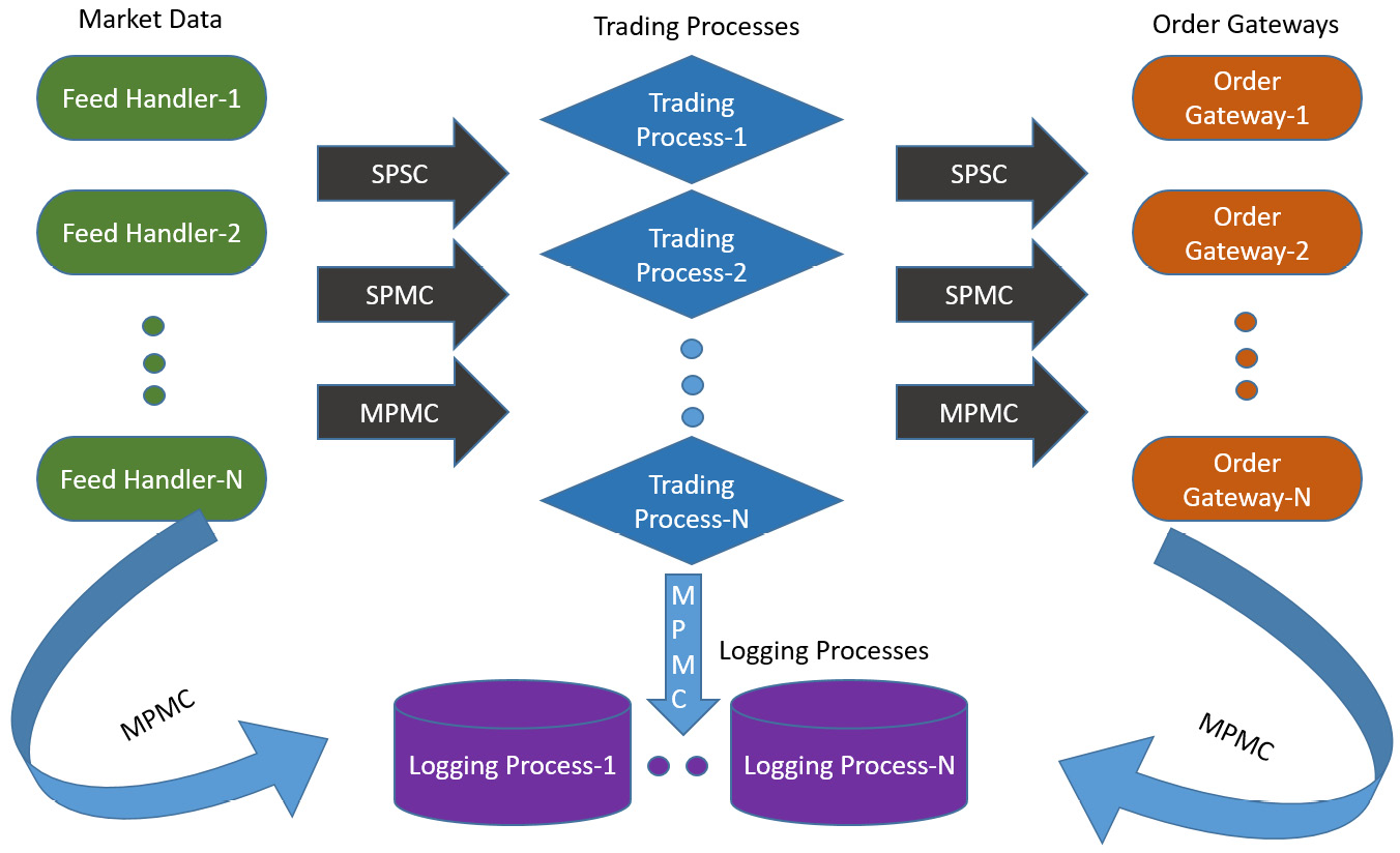
Figure 6.2 – The layout and use of different types of lock-free queues (SPSC, SPMC, and MPMC) in a complete HFT ecosystem

In this section, we discussed traditional computer science concurrency/synchronization mechanisms and why they are needed in multi-threaded applications. We then looked at why the use of locks is inefficient for HFT applications. Finally, we designed a lock-free data structure to be used in the presence of multiple producers of data and multiple consumers of that data and saw how that fits into an HFT ecosystem. In the next section, we will look at another important topic concerning all applications in general, but especially relevant to HFT applications – memory allocation during the course of an HFT application's life cycle.

Pre-fetching and pre-allocating memory

In this section, we will look at two things when it comes to accessing and allocating memory used by HFT applications mostly from the perspective of improving memory access and allocation latencies, especially on the critical path.

We will start off by discussing the hierarchy of memory – all the way from memory with super-fast access but that is expensive and limited in capacity, to those offering super-slow access but cheaply and of huge capacity. We will also discuss some strategies to design HFT applications to aim for optimal memory access latencies.

The other topic of discussion will be how dynamic memory allocation works, why dynamically allocating memory on the hot path is inefficient, and what techniques are employed to extract maximum performance without sacrificing too much of the flexibility that dynamic memory allocation allows.

Memory hierarchy

First, we will discuss the memory hierarchy in modern architecture. We will start from the storage closest to the processor, which has the lowest access latencies (but the highest cost and lowest storage capacity) and move further out from processor registers to various levels of caches to main memory (RAM) and then finally to the disk storage where applications reside before they are loaded into memory on startup. Note that these numbers vary from architecture to architecture and processor to processor and are in a constant state of evolution, so these are meant to be rough approximations of what to expect and are likely to change in the future.

First, let's look at a diagram that describes the pyramid of memory hierarchy from fastest, smallest, and most expensive at the top to slowest, largest, and least expensive at the bottom:

Figure 6.3 – Memory hierarchy in a modern architecture

As we move from the bottom to the top, the memory/storage options become faster, lower in capacity, and more expensive.

Processor registers

Processor registers have the fastest possible access (usually 1 CPU cycle). The processor register banks can hold up to a few bytes in size per register.

Caches

After the processor registers comes the cache bank, which comprises a few different cache levels. We will discuss those here in order from fastest (and smallest) to slowest (and largest).

L0 cache

Level 0 (L0) cache – this is accessed after the processor registers. The L0 cache is around 6 kilobytes in size.

L1 cache

Level 1 (L1) caches (the instruction and data caches) is 128 kilobytes in size. Access times are around 0.5 nanoseconds for the data cache and 5 nanoseconds for a branch misprediction for the instruction cache. Branch prediction is an advanced computer architecture feature where, based on previous access patterns, the processor/OS tries to guess which code path will be taken next. When it guesses the path correctly, it can pre-fetch the code before it is needed, thus speeding up access and execution when it is finally needed. Since it is a guess, sometimes it is incorrect, which is known as branch misprediction. We will not dive into too many details on branch prediction since that is outside the scope of this book.

L2 cache

Level 2 (L2) caches - instruction and data (shared) – sizes vary here but can range from 256 kilobytes to 8 megabytes. L2 cache access takes around 5-7 nanoseconds.

L3 Cache

Level 3 (L3) shared cache – L3 caches can vary in size from 32 to 64 megabytes. The L3 cache is the largest but also the slowest, with access times of around 12 nanoseconds. The L3 cache can exist on the CPU itself, however, there are L1 and L2 caches for each core, while the L3 cache is more of a shared cache for all cores on the chip.

L4 Cache

Level 4 (L4) shared cache – these can vary from 64 to 128 megabytes. Access times are around 40 nanoseconds.

Main memory

Main memory (primary storage) – this varies in size from 16 to 256 gigabytes. Access times are around 60 nanoseconds. Non-Uniform Memory Access (NUMA) machines experience non-uniform access times. NUMA is an advanced concept where in a multi-threaded environment the access times depend on the memory location relative to the processor, but diving into NUMA is outside the scope of this book.

Disk storage

Disk storage (secondary storage) – This goes up to terabytes in size. For solid-state storage, access speeds are around 100 microseconds, and for non-solid-state storage, around 300 microseconds.

Inefficiencies with memory access

In the previous section, we discussed the memory hierarchy and latencies incurred when fetching data from the different storages – basically, when an application requests a data for the first time, it might not be available in the registers or the caches and possibly (we will discuss why we use the word possibly in the Pre-fetching based alternatives to boost performance section) not even in the main memory, in which case it is loaded from disk to main memory (incurring the 100-300 microseconds latency), then from main memory to the L0 to L4 caches. Data is not loaded a few bytes at a time but one or few pages (a few kilobytes) at a time, so subsequent references to the same data (or data residing at a memory address close to that data) lead to cache hits and experience significantly lower access latencies.

So, the worst-case access time latencies are incurred when we experience a miss at the faster storage levels and must go to the slower storage, fetch it, cache it into the faster storage, and then access the requested data, yielding a few hundred microseconds in access latency.

The best-case scenario is when the data is already present in the L0/L1 cache and access times drop to less than a nanosecond. The average-case latency (referred to as Average Access Time) (AAT)), which is what we are really trying to optimize, is the average of access times over the course of an application's life cycle.

Let's say we have a hypothetical setup where the main memory has an access time 60 nanoseconds, the L1 cache has an access time of 0.5 nanoseconds but a miss rate of 10%, the L2 cache has an access time of 5 nanoseconds with a miss rate of 1%, and the L3 cache has an access time of 12 nanoseconds and a miss rate of 0.1%, then the AAT will be as follows for the different scenarios:

• No cache: AAT-no-cache = 60 nanoseconds
• L1 cache: AAT-L1 = L1-hit-time + (L1-miss-rate * AAT-no-cache) = 0.5 + (0.1 * 60) = 6.5 nanoseconds
• L2 cache: AAT-L2 = L1-hit-time + (L1-miss-rate * (L2-hit-time + L2-miss-rate * AAT-no-cache)) = 0.5 + (0.1 * (5 + 0.01 * 60)) = 1.06 nanoseconds
• L3 cache: AAT-L3 = 0.5 + (0.1 * (5 + 0.01 * (12 + 0.0001 * 60))) = 1.012 nanoseconds

The takeaway here is that applications that have memory access patterns that lead to a lot more cache hits (and thus fewer cache misses) will have significantly better performance in terms of accessing memory than an application that has access patterns that lead to a lot more cache misses (and thus fewer cache hits).

Pre-fetching based alternatives to boost performance

In the previous section, we discussed how cache hits affect memory access performance. So, to get the most out of cache performance, HFT application developers need to focus on writing cache-friendly code, the most important aspect of which is the principle of locality, which basically describes why related datasets placed near each other in memory allow for more efficient caching. You must be aware of how big each of the caches are, how much data fits in a cache line, and cache access times for the specific architecture where the HFT ecosystem lives.

Temporal locality

Temporal locality refers to the principle that given that a certain memory location was accessed, it is highly likely that the same location will be referenced/accessed again soon. So based on that principle, it makes sense to cache data that was recently accessed since there is a good chance that it will be accessed again and likely that it will still be cached at that point.

Spatial locality

Spatial locality refers to the principle of placing related pieces of data close to each other. Typically, memory loaded into RAM is fetched in large chunks (larger than what the application requested) and similarly for hard disk drives and CPU caches. The reasoning here is that application code is often executed serially (instead of jumping around randomly across memory addresses) and so the program will most likely require the data from the large chunk that was fetched in the previous instance. Thus, it is likely to produce cache hits or memory hits instead of having to fetch it from disk.

Appropriate containers

It is important to think carefully about the containers being used when writing cache-friendly low-latency HFT code. A quite simple example often presented is the choice between the C++ Standard Template Library (STL) vectors and lists. While both might appear to be serving similar purposes from the API perspective, the elements of a vector are saved in contiguous memory locations and they are much more cache friendly when it comes to accessing them compared to lists where the elements are not necessarily stored in contiguous memory and often all over the place in memory. Here, the principle of spatial locality kicks in and causes vector element access to perform significantly better than list element access.

Cache-friendly data structures and algorithms

This is a generalization of the previous point – when designing data structures and algorithms, it is important to be cognizant of cache and cache performance and try to tailor the design in a way that maximizes the use and performance of the cache, especially for HFT applications.

Exploit the implicit structure of data

Another simple example that is often presented when discussing spatial locality is the classic 2D array, which can be column-major (where elements of a column are next to each other in memory) or row-major (where elements of a row are next to each other in memory). We should consider this and access the element accordingly – for example, for column-major 2D arrays, accessing elements in the same column is much better than accessing elements in the same row, and the reverse is true for row-major 2D arrays. Data that is fetched from the main memory and cached in the cache bank is fetched in units of blocks. So, when a certain element of a matrix is accessed, elements near it in memory locations are also fetched and cached. Exploiting this ordering allows us to perform operations with fewer memory accesses because computations that need to access the subsequent elements already find them in the cache line.

Avoid unpredictable branches

Modern compilers, processor pipelines, and architecture are extremely good at prefetching data and reordering code to minimize memory access delays. But one place where they suffer in performance is if the critical code contains unpredictable branches since it is impossible to pre-fetch data and exploit temporal or spatial locality and pre-fetch data. This therefore leads to significantly more cache misses compared to code without a lot of unpredictable branches.

Avoid virtual functions

Virtual functions in the context of C++ are something that we try to avoid when writing low-latency HFT software in general, mostly because they make a lot of especially important compiler optimizations impossible simply because the compiler cannot determine which method implementation will get called at compile time, so it cannot inline the methods and processors cannot pre-fetch data. This results in a lot more cache misses during lookup if the specific method is not called often (otherwise at least the method body is likely to be cached and will not incur cache misses). The presence of virtual functions is not the biggest problem when it comes to cache friendliness, but still, this is something to be cognizant of.

In the next section, we will look at another topic related to memory allocation and access – dynamic memory allocation. Dynamic memory allocation is quite common in complex large-scale applications, so it is important to build a good understanding of that concept. You should build a good understanding of the fact that there are multiple steps involved each time a dynamic memory allocation operation is invoked and that can have performance penalties for HFT applications.

Dynamic memory allocation

Dynamic memory management is an excellent feature that has existed since the beginning of C – it allows applications to manage (allocate/move/deallocate) memory blocks of dynamic sizes determined at runtime. The actual internal implementation and performance impact, however, makes it less than ideal for extremely low latency HFT applications that need very tight (low variance on latencies on operations) performance. The memory allocated during dynamic memory allocation lives on the heap segment and when memory is freed, it is returned to the heap. However, in practice working with dynamic memory management is non-trivial and small mistakes in the application implementation can lead to subtle memory leak issues and performance issues on the critical path.

Steps in dynamic memory allocation

The OS maintains the free heap memory blocks using two linked lists – one is a freed list of heap memory blocks that are not currently allocated, and the other is an allocated list of heap memory blocks. When a request comes in for a new memory block, it traverses the freed list till it finds a memory block that is large enough to service the request, then moves part or all of the memory block from the freed list to the allocated list and returns the now allocated memory address back to the caller.

Over the course of a program's life cycle there can be any number of allocations and deallocations of random amounts in random orders. Due to these operations, the freed list can have holes when previously allocated memory is returned to the free list in between still allocated memory blocks. A new request for dynamically allocated memory can return something from one of the holes. This concept of the freed heap block list developing holes is known as memory fragmentation. In some rare cases it is possible for a lot of fragmentation and due to the presence of too many holes, memory is wasted and the holes cannot be used to satisfy dynamic memory allocation requests because each hole individually might be too small to satisfy the request. There are some techniques and strategies that the allocator invokes periodically to collect and consolidate such chunks to prevent heap fragmentation, but covering those is outside of the scope of this chapter.

Memory leaks are another problem for dynamic memory allocation, whereby a memory block is allocated but remains unused and is never freed by the application and hence not returned to the free pool. This is known as a memory leak and it causes memory usage to balloon, along with worsened performance due to the gigantic memory footprint, and might even cause the OS to terminate the process that is leaking memory and/or starve all processes that need dynamic memory to be allocated.

To summarize this section, dynamic memory management introduces application complexity, the potential for bugs, has an overhead and latency (due to the tracking/updating of the linked lists tracking the memory blocks), and can have performance issues due to memory fragmentation. The performance implications make dynamic memory management less than ideal for HFT applications.

Pre-allocation-based alternatives to dynamic memory allocation

In this section, we will investigate some alternatives when it comes to dynamic memory management. Here we want to preserve the flexibility of being able to allocate and deallocate an arbitrary number of elements at runtime, but we will try to see how we might be able to achieve this without encountering the performance issues of the dynamic memory management provided by the OS.

Some solutions to the dynamic memory management problem are listed here.

Limit memory to stack

One obvious solution is to limit dynamic memory allocation on the heap. What that means is that if something can be allocated on the stack, that should be the preference. Simple techniques such as having an upper bound on the number of elements and having a local variable on the stack to handle up to that number of elements can help eliminate the drawbacks of using dynamic memory allocation anytime an unknown number (at compile time) of elements could be needed.

Memory pools

If the type of object is known (as is quite frequently the case; for example, an Order object type that contains details about an order in market data, such as price, side, and quantity), it is often much more efficient to create a memory pool, allocate a huge block of memory, and manage the memory in software ourselves. Since the type and size of the object are known, the actual memory pool implementation can be made generic but super-efficient by using templates. Also, since the size of each element, we do not have to worry about holes/memory fragmentation. Additionally, we can use a LIFO stack-style deallocation/allocation scheme instead of a linked list, which is likely to give much better cache performance as well. Finally, using huge pages can help with the TLB translation efficiency in scenarios where we expect to create many specific kinds of objects.

In this section, we addressed details around accessing memory on modern architectures and OSs – the design of memory hierarchy, the inefficiencies of normal access patterns, and some techniques to maximize performance for HFT application requirements. We also discussed dynamic memory allocation, the drawbacks of using it on performance-critical paths, and techniques to use it without impacting performance for HFT applications.

Summary

We discussed the implementation details of various computer science constructs such as context switching, synchronization, and concurrency primitives. We also discussed the implications that these features have on HFT applications and found that often the default behavior that works best for most applications is not the optimal setup for HFT applications.

Finally, we discussed approaches/tools/techniques/optimizations for optimal HFT ecosystem performance. We hope this chapter provides you insight into advanced HFT optimization techniques and their impact on the HFT ecosystem's performance.

For developers and traders that want to build HFT systems and trading strategies, it is imperative that you understand the use of these HFT optimization techniques. The biggest edge in HFT comes from ultra-low latency algorithms/software and to be able to compete in that space, you will need to employ these techniques.

The next chapter will continue on the subject of HFT optimization technologies/techniques. We will discuss HFT optimizations that apply to kernel bypass technology, networking, logging, and performance measurement.