
Automating Analysis and Extending Capabilities
Information in this Chapter
Introduction
If you have been working straight through this book, you should be able to perform a successful examination using only the tools and techniques discussed in the previous chapters. This chapter focuses on expanding your analytical capabilities in two distinct ways. First, we examine tools that build upon the programs and concepts from the previous chapters and, in doing so, provide additional benefit to the examiner. These benefits include a more integrated working environment, collaboration possibilities, extended searching and filtering capabilities, and automation. The second part of the chapter deals with extended concepts of temporal analysis. Because timeline generation and analysis are such an integral part of many forensic examinations, it is imperative to have a good understanding of how to extract more meaning from time data.
Graphical Investigation Environments
Many of the tools examined in previous chapters are command line or console based, which can be a tremendous advantage in various scenarios and provide a great deal of flexibility. However, some workflows are better suited to a graphical environment. Advantages of using a graphical examination platform include integrated case management, built-in keyword searching, and greater continuity when examining between the various file system layers. The prime example of the open source graphical forensic environment is the venerable Autopsy browser, created by Brian Carrier as a visual front end to the Sleuth Kit tools. The Autopsy browser does not provide any capabilities above and beyond those provided by the command line Sleuth Kit tools but does provide a more comfortable environment for examiners who are primarily GUI users. The next two sections discuss two graphical investigation environments that do provide a host of additional examination capabilities: PyFLAG and the Digital Forensics Framework.
PyFLAG
PyFLAG is the Python-based Forensics and Log Analysis GUI created by Michael Cohen and David Collett to support unified examination of disparate data types often encountered in modern forensic examinations [1]. Because PyFLAG is a Web-based, database-backed application, a user generally just needs a Web browser to perform an examination. Being a Web/database application gives PyFLAG several advantages over more traditional forensic utilities, which tend to be single-user/single-computer bound. A PyFLAG instance can support multiple users on a single case or multiple users working on different cases in parallel. As any examiner can tell you, when it rains, it pours, so having the ability to scale up the number of examiners that can work on a given case at one time can be incredibly valuable. In addition to the server model, PyFLAG has some other features that make it an interesting tool for an examiner using open source tools.
Virtual File System
Much like the unified file system concept common to Unix and Linux systems (as discussed in Chapter 5), PyFLAG features a unified Virtual File System (VFS) for all objects under examination. PyFLAG refers to each of these items as inodes. Each item loaded into the PyFLAG database receives a PyFLAG inode, in addition to the internal file system metadata address it may already have. This means that any number of file system images, network traffic captures, standalone log files, and even streams of unstructured data may be loaded under the same virtual root and subsequently processed with PyFLAG.
Additionally, as an examination using PyFLAG proceeds it is not uncommon to discover nested files (such as files inside of archives, or files recovered via carving or extracted from a network packet capture). These nested files will be allocated a PyFLAG inode chained under their parent item. These chained inodes will be indicated by a pipe character (|).
Scanners
PyFLAG’s scanners are discrete modules with a specific task. A scanner will run over objects loaded into the VFS and perform a function. For example, the PstFile.py scanner will run over inodes loaded into the VFS, determine if they are an Outlook PST, and process them accordingly. This processing populates the VFS with inodes referencing any discovered discrete items inside of the PST, which are then rescanned with any additional loaded scanners. Using discrete scanners coupled with the inode creation and nesting mentioned earlier can enable an examiner to fairly rapidly gain deep knowledge of the true contents of the file system in question.
SQL Queries
The bulk of the PyFLAG GUI is simply a front end to submitting SQL queries to the back-end database, and then formatting and displaying the results. One nice aspect of this division is that the database can be queried and manipulated directly, without the necessity of the browser. Indeed, many of the more advanced functions of PyFLAG require direct database interaction.
If you are not familiar with SQL queries, however, PyFLAG should still be usable and may, in fact, assist you in learning SQL. On each set of responses displayed by the PyFLAG GUI that are results of a SQL query, there will be a “SQL Used” Icon that resembles a hand holding some traditional database icons. Clicking this will display the SQL query the GUI issued to the database to generate the page in question.
Additionally, PyFLAG uses SQL to do all of its display filtering. In any of the filtering dialogues, you can enter SQL directly or you can use the provided “helper” functions that display available tables and operators.
Keyword Searching and Indexing
PyFLAG does not offer “on demand” keyword scanning. This isn’t necessarily a shortcoming, as performing a full file system scan for each keyword is incredibly time-consuming on large file systems. Instead, PyFLAG offers indexed searching. PyFLAG builds an index based on a dictionary file, which allows for very fast searching. However, it only builds this index when a new source is loaded into a case. As the PyFLAG dictionary is empty after installation, this effectively means that unless the examiner takes steps to set up a dictionary, keyword searching won’t be possible.
The PyFLAG FAQ contains a handy set of commands to populate the index with a large number of keywords sourced from the wordlist file included for spellcheck support on most Linux distributions:
~/pyflag$ grep -E ...+ /usr/share/dict/words > keywords.txt
~/pyflag$ pyflag_launch ./utilities/load_dictionary.py keywords.txt
This retrieves all three-letter or longer words and loads them into the PyFLAG database. Note that this technique can be extended to load any arbitrary set of keywords for indexing.
Carving and Advanced Carving
PyFLAG supports file carving in a fairly novel way, through use of the VFS. Using simple header/footer signature carving, PyFLAG carvers generate VFS inodes corresponding to the location and run length of the corresponding hit. The only overhead from carving is the time and cycles required to perform the carving rather than the heaps of disk space required for a standard carving operation. Additionally, PyFLAG carvers will run over all inodes present in the VFS, to include inodes generated by scanners. Given this, it is possible to extract embedded files from within archives without performing the intermediary extraction and decompression phases out to disk.
PyFLAG also supports a handful of advanced carvers that use built-in knowledge of the file structures they are carving. The three advanced carvers currently supplied with PyFLAG are for PDFs, JPEGs, and ZIP archives.
Log Analysis
As the name belies, PyFLAG is equally intended to be used for log analysis as well as file system forensic analysis. Because logs entries are stored in the PyFLAG database and are indexed in the same manner as all other content, keyword searches across the database will produce log results in addition to file system results. PyFLAG currently has native knowledge of the Windows binary event log format, IIS logs, Apache Logs, and Linux IPTables logs, but also supports generating log templates based on a source log file.
Network and Memory Forensics Support
While an exploration of these capabilities is outside the scope of this book, it is important to be aware that one of PyFLAG’s greatest strengths is its ability to intelligently parse various application-layer networking protocols. Network protocols currently supported in PyFLAG include HTTP Web traffic, SMTP and POP mail transfer, IRC chat, and VOIP telephony.
PyFLAG also interfaces with the Volatility framework, an open source framework for performing forensic analysis memory images from Windows and Linux systems. Items recovered from network or memory captures will be populated into the VFS and can be processed further using any of the appropriate scanners.
An excellent walkthrough of performing a unified investigation using PyFlag is available in Michael Cohen and AAron Walters’ write up from the 2008 Digital Forensics Research Workshop Forensics challenge [2]. To demonstrate basic usage of PyFLAG for file system forensic analysis, we will install the application and explore some of the features available using Lance Mueller’s first Forensic Practical Image, available at http://www.lancemueller.com/blog/evidence/WinXP2.E01.
Installation
PyFLAG installation is a bit more involved than many of the other packages we have used up to this point. It has many components and is not currently included in any package management systems. In addition, the most recent version is only available via the darcs source code management system. We will need to start out by making sure we have all the dependencies required for PyFLAG’s operation. The install document (available online at http://www.pyflag.net/pyflag/INSTALL or with the PyFLAG source) states the following packages are required and handily provides the Debian/Ubuntu package names:
Additionally, we will need the “mysql-server,” “python-sqlite,” and “python-pyparsing” packages. We have some of these already, but requesting them again will not hurt anything, so we can install all of these (and their dependencies, and so on) in one shot with the following command:
sudo apt-get install build-essential python-dev libz-dev libmagic-dev python-mysqldb python-imaging python-pexpect python-dateutil python-urwid mysql-server python-sqlite python-p6
PyFLAG can provide additional, optional functionality if the following packages are installed:
• geoip (libgeoip-dev) for Maxmind GeoIP support
• libjpeg (libjpeg62-dev) for Advanced JPEG Carving support
• afflib for AFF image support
Because we installed AFFLIB and LibEWF from source in Chapter 2, we can skip these and only install the other packages using:
sudo apt-get install libgeoip-dev libjpeg62-dev clamav-daemon
With all the prerequisites installed, we can fetch the current development branch of the PyFLAG source code. PyFLAG uses darcs revision control software. If you don’t have this installed, you can rectify this with apt-get. We can fetch a copy of the current source to work with using the following command:
darcs get --partial http://www.pyflag.net/pyflag
Once the command completes we will have a new directory named pyflag in our current directory. We will need to move into this directory and execute the included “autogen.sh,” which will set up the build environment.
sh autogen.sh
This will create the configure script and associated files, so once this is completed a standard build will complete the process:
./configure
make
sudo make install
The next step is to start up PyFLAG.
user@ubuntu:~/source/pyflag$ sudo pyflag
Checking schema for compliance
31172(Warning): Error: Unable to connects - does the DB Exist?: (1049, "Unknown database ’pyflag’ ")
31172(Warning): Error: Unable to connects - does the DB Exist?: (1049, "Unknown database ’pyflag’ ")
31172(Infomation): Serving PyFlag requests on http://127.0.0.1:8000
Note that the errors are completely normal—the “pyflag” database does not exist the first time you run PyFLAG. Setting this up is the first thing we have to do.
Once we open a Web browser and navigate to the provided URL, we will be prompted to initialize the database. If we check the “Upgrade the database?” box and click Submit, PyFLAG will build the “pyflag” database using the appropriate schema.
Before continuing further, we need to confirm (and possibly change) some PyFLAG configuration data. There are two primary configuration directives of concern: uploaddir and resultdir. These determine where PyFLAG looks for input files and where it places output files. Because PyFLAG will not be able to read or write to the file system outside of these directories, ensure that they exist and make sure to place any data you plan on analyzing with PyFLAG in the uploaddir directory.
Usage
Once the database is created and our configuration options are acceptable, the next step is to start a new case (Case Management -> New Case). Give your case a memorable name and click Submit.
Next, we will need to add an image file to process using PyFLAG. Select Load Data -> Load IO Data Source. You should see the screen shown in Figure 9.1.

Figure 9.1 PyFLAG—adding an image file.
Using our example image shown in Figure 9.1, we will select “EWF” as the IO Subsystem. After hitting Submit, we see the screen in Figure 9.2. Note that PyFLAG performs some preliminary analysis of the loaded data, hinting at the content in the red highlighted text.

Figure 9.2 PyFLAG—file system parsing.
Because this is a file system image, we will select “Sleuthkit” as the file system type. This tells PyFLAG what driver to use to analyze the structure of the data source we are loading. Before proceeding, we will need to provide a VFS Mount Point for the data source. This is like creating a mount point when mounting a volume on a Linux system. We can put whatever we would like here, but it is best to choose something relevant to the source material, such as “WinXP2.”
Once the file system driver loads, you should get a file browser view similar to Figure 9.3.

Figure 9.3 PyFLAG—file system browsing.
From here we can browse through the file system using the GUI, export files, and so on. Before we do that, though, we can exercise some of PyFLAG’s more interesting capabilities. Selecting Load Data -> Scan Filesystem takes us to the screen shown in Figure 9.4.

Figure 9.4 PyFLAG file system scanners.
This is the main configuration panel that determines which scanners are run against the VFS (or a subsection defined under the “Scan Files” entry). Each entry shown is a category, and clicking on the tool icon to the left of each lets an examiner drill down and enable or disable specific scanners. Once we are done setting which scanners we want, we can click “Submit” to kick off the scanning process. This yields the display seen in Figure 9.5.

Figure 9.5 PyFLAG scanner progress.
After scanning is complete, you are returned to the file system browser. Any new inodes generated by the scanner will be populated into the VFS automatically.
A frequent task in forensic analysis is examination of files of a specific type—only images, for example. PyFLAG has a function that displays all files by type under Disk Forensics -> Browse Types. This simply displays all files on the system for which a type was able to be determined. We can utilize the filtering capabilities of PyFLAG to restrict this to only JPEG images, for example. Selecting the Filter icon brings up the page shown in Figure 9.6.

Figure 9.6 PyFLAG filtering.
We can use the “Column” and “Operators” drop-downs to generate a Filter without knowing any SQL. Simply select the column or operator of interest, position the cursor in the Search Query field, and select “Insert.” When the query is completed, click “Submit.” See Figure 9.7 for a subset of the resulting JPEG-only output.

Figure 9.7 PyFLAG—JPEG filtering results.
PyFLAG has another method for viewing files of a specific type under Disk Forensics -> Feeling Lucky. These are canned sets of queries useful for retrieving specific sets of data. In Figure 9.8, this was used to retrieve all graphics files from the file system.

Figure 9.8 PyFLAG—all images search.
As mentioned before, we can use the “SQL Used” button to force PyFLAG to “show its work,” so to speak. The segment that follows is the SQL statement used in the graphics query in Figure 9.8.
select inode.inode_id as ’Thumbnail’,’inode’.’size’ as ’Size’,file.link, concat(file.path,file.name) as ’Filename’ from ’inode’ join ’file’ on ’inode’.inode_id = ’file’.inode_id where ((1) and (( ’inode’.’inode_id’ in (select inode_id from type where type like ’%image%’)) and ’inode’.’size’ > ’20000’)) order by ’inode’.’size’ desc
Note that this is but a small sampling of what you can do with PyFLAG. Many more extensive tutorials are available on the PyFLAG wiki.
Digital Forensics Framework
ArxSys’s Digital Forensics Framework (DFF) is a relative newcomer to the world of forensic GUIs, but it appears to be receiving a lot of active development at a fairly rapid pace [3]. At this time it does not have many of the features present in PyFLAG, but it does present a somewhat cleaner GUI and is quite simple to build and install on Linux, OS X, and Windows. In addition, it is quite extensible via scripts and plugins so a sufficiently skilled examiner can overcome any shortcomings that are discovered.
Virtual File System
Much like PyFLAG, DFF also creates a Virtual File System under which all subsequent items are loaded. DFF refers to unique items as nodes. The core of the DFF application is tasked with handling the creation of VFS nodes in memory. All display tasks are handled by a GUI layer, and populating nodes with data is handled by modules. The Virtual File System is viewed as a tree structure in the DFF GUI, with all nodes appearing as children under the root (/ ) or as children of other nodes.
Modules and Scripts
DFF modules are similar to PyFLAG’s scanners. A module performs a discrete task and populates a node with the output of that task. The current version of DFF (0.8 at the time of this writing) comes with many modules that perform various tasks, including processing cell phone memory dumps, performing hash comparisons, viewing movies and images, and generating statistics about a node or set of nodes. Because all “analysis tasks” in DFF are performed via modules, the exposed application programming interface (API) has a great deal of functionality available. Additional modules can be written in C++ or Python. In addition, scripts can be generated on the fly using the built-in Python scripting engine.
GUI and Command-Line Capabilities
One of the strongest features of the Digital Forensics Framework is the clean, simple GUI. The familiar three-pane layout is a paradigm used by many GUI applications so even a novice should not have much trouble getting oriented in the application. Additionally, all functions performed via modules from the GUI can also be performed via the DFF shell. The DFF shell can be launched from within the GUI or can be used standalone. This allows the examiner to use the same tool whether she is connecting via a remote shell or sitting at a local desktop.
Installation and Prerequisites
DFF is available via a binary installer package for most Linux distributions and Windows and can be compiled from source on Windows, Linux, and OS X systems. In this example, we compile DFF 0.8.0 from source.
As always, first we need to install the program’s dependencies. DFF’s GUI is based on the QT4 library, so we will need to install a host of packages related to this. The following command will get us all the packages we need to build DFF successfully.
user@ubuntu:~$ sudo apt-get install swig1.3 cmake python-qt4-dev pyqt4-dev-tools qt4-qmake libqt4-dev libqscintilla2-5 libqscintilla2-dev python-qscintilla2 python-magic python-qt4-phonon
DFF uses the cmake build system, so to start the process off we run “cmake” in the DFF’s unpacked source directory.
user@ubuntu:~/source/dff-0.8-src$ cmake .
This will generate the makefiles we need to compile. Once complete, we can run make and then make install.
user@ubuntu:~/source/dff-0.8-src$ make
...
user@ubuntu:~/source/dff-0.8-src$ sudo make install
Usage
We will use the same image as before to explore the usage of DFF (WinXP2.E01). At this point, DFF does not support Expert Witness Format images; however, as demonstrated in Chapter 2, we can create a virtual mount point for the EWF container and expose the content as a “raw” image, which DFF can process using the following series of commands.
First we’ll create a mount point for the container:
user@ubuntu:~$ mkdir ~/mnt
user@ubuntu:~$ mkdir ~/mnt/ewf
Next we will mount the EWF container:
user@ubuntu:~$ mount_ewf.py ~/images/WinXP2.E01 ~/mnt/ewf/
Using libewf-20100226. Tested with libewf-20080501.
Finally, we can confirm a proper mount by listing the directory we mounted the EWF to:
user@ubuntu:~$ ls -lath /home/user/mnt/ewf/
total 2.0G
drwxr-xr-x 3 user user 4.0K 2010-11-26 09:26 ..
dr-xr-xr-x 2 root root 0 1969-12-31 16:00 .
-r--r--r-- 1 root root 2.0G 1969-12-31 16:00 WinXP2
-r--r--r-- 1 root root 284 1969-12-31 16:00 WinXP2.txt
With this set up, we can start up DFF. We will pass the “-g” argument to tell DFF to start the GUI—without this flag, DFF defaults to shell operation.
user@ubuntu:~$ dff -g
Once the GUI comes up, the first thing we need to do is have it read in our image file. To do so, we will select “Add Dump” from the File menu (Figure 9.9). DFF uses “Dump” to refer to a bitstream image of a device, as opposed to a physical device.

Figure 9.9 DFF adding image file.
After browsing to and opening our FUSE-mounted image file (/home/user/mnt/ewf/WinXP2 in our example), we get Figure 9.10. Note that adding the dump did just that, nothing more. We need to tell DFF to process the dump file further.

Figure 9.10 DFF raw image view.
We can examine the attributes of the file on the right to determine that it is an NTFS volume. To process the NTFS structures in the dump, we can select Modules -> File System -> NTFS (Figure 9.11).

Figure 9.11 DFF NTFS parser.
The NTFS parsing module has a few configurable options, as seen in Figure 9.12. Optional fields are off by default—the checkbox to the right enables editing them.
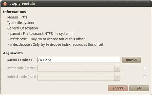
Figure 9.12 DFF NTFS parsing options.
We provide a name for the node we are creating with this module (/WinXP2) and hit “OK.” The Task Manager pane at the bottom of the window should provide a status update as the NTFS processing tasks proceed. Once completed, we are presented with a standard tree file browsing structure, which we can use to examine the file system interactively. For an example of navigating DFF using the thumbnail view, see Figure 9.13.

Figure 9.13 DFF file system browsing.
One of the interesting modules included in DFF is the Fileschart module (Modules -> Statistics -> Fileschart). This performs cursory file analysis of all nodes and displays a graphical overview of the types of files present in the VFS (Figure 9.14).

Figure 9.14 DFF file type statistics.
DFF also includes a carving module. Currently the carving mechanism used is a simple header search, and the types of files supported are fairly limited. Figure 9.15 shows an active file carving process.

Figure 9.15 DFF carving.
Carved files will be added to the VFS under the node they were found in under a new directory named “carved” (Figure 9.16).

Figure 9.16 DFF-carved files.
DFF contains a number of native viewer modules—an image viewer for graphics files, a movie player for video files, and a text viewer for text files. Unknown or binary files will be displayed using the hexedit module. Among hexedit modules features is the ability to search the file content for hexadecimal, ASCII, or Unicode strings. In Figure 9.17 we searched for “hbin” in the Adminstrator’s NTUSER.DAT file and received 91 results. Clicking on the address of each results in the Offset pane in the lower right will jump to that hit.

Figure 9.17 DFF Hex Editor search.
The hexedit module also allows the user to highlight and bookmark selected segments of data. In Figure 9.18 we have highlighted and bookmarked a registry key of interest.

Figure 9.18 DFF bookmarking.
The DFF unzip module (under archive) allows an examiner to examine the contents of a zip archive without extracting data first. In Figure 9.19 we launched the unzip module by right clicking on a Zip archive and selecting the “unzip” module from the context menu.

Figure 9.19 DFF unzip module.
The archive content is added as a child node of the Zip archive under the VFS. We can now navigate down into the archive and examine the content, including the embedded time stamp (shown in Figure 9.20).
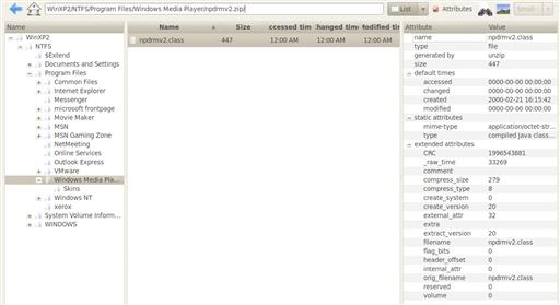
Figure 9.20 DFF zip content view.
Automating Artifact Extraction
One of the constant challenges of forensic analysis is the amount of setup required before true analysis can be performed. If you are simply looking to identify and extract a specific file type, you still need to identify the partitions on image, identify the file systems, access their contents, locate files in question, and so on. The majority of this preliminary work is not interesting and not directly relevant to the purpose of the exam. The goal of automating artifact extraction is to reduce the amount of setup required before real work can begin.
Fiwalk
Fiwalk is a library and suite of related programs designed to automate much of the initial file system analysis performed during a forensic examination [4]. The name comes from “file & inode walk,” which is effectively what the program does. Fiwalk’s output is a mapping of a disk’s file systems and contained files, including embedded file metadata if requested. The goal of the fiwalk project is to provide a standardized XML description language for the contents of a forensic image file and to enable more rapid processing of forensic data.
Because fiwalk inherits file system analysis capabilities from the Sleuth Kit, it is able to support any partition, volume, and file system structures the Sleuth Kit is capable of reading. In addition to its standard XML output, fiwalk can provide output in human-readable text, Sleuth Kit bodyfile format, the ARFF format used by the open-source Weka data mining system, and plain CSV for import into a spreadsheet program.
We can demonstrate the use of fiwalk by using it to generate a Forensic XML document describing the content of the ubnist1.casper-rw.gen3.aff file from Digital Corpora.
fiwalk -X ubnist1.gen3.xml ubnist1.casper-rw.gen3.aff
The resulting output is a 2.1-Megabyte XML document containing 2533 “fileobject” elements. An example fileobject element (for /etc/hosts) is shown here.
<fileobject>
<filename>etc/hosts</filename>
<partition>1</partition>
<id>65</id>
<name_type>r</name_type>
<filesize>243</filesize>
<alloc>1</alloc>
<used>1</used>
<inode>23065</inode>
<meta_type>1</meta_type>
<mode>420</mode>
<nlink>1</nlink>
<uid>0</uid>
<gid<0</gid>
<mtime>1231268387</mtime>
<ctime>1231268387</ctime>
<atime>1230469854</atime>
<libmagic>ASCII English text</libmagic>
<byte_runs>
<run file_offset=’0’ fs_offset=’528486400’ img_offset=’528486400’ len=’243’/>
</byte_runs>
<hashdigest type=’MD5’>0a936719a10e067bab6fd92391776225</hashdigest>
<hashdigest type=’SHA1’>59bcce3e528094e1c7d09d32af788a5eb0f9960b</hashdigest>
</fileobject>
We can see that this element contains all the information we need to know about the file, including the three stored time stamps, ownership data, two hashes, a “libmagic” determination of the content of the file, and the location in the image where the file’s content resides.
Fiwalk-based Tools
The main fiwalk program is written in C in the interest of speed. However, the fiwalk project also provides a Python module (fiwalk.py) so that forensic applications leveraging fiwalk’s capabilities can be developed quickly and simply. To demonstrate this, several demonstration programs that use fiwalk.py are included. These can be used as is or as a basis for additional programs leveraging the fiwalk core.
One example is iredact.py, which is a disk redaction program designed to enable the intelligent removal of files meeting specific criteria from a disk image. The idea is to remove sensitive or otherwise nonshareable information from a disk image prior to making this image available to third parties. Altering a forensic image is always a fraught with peril, but because iredact.py is designed with forensic needs in mind, it avoids oversterilization or disturbing unallocated data.
Redaction is controlled by sets of condition:action pairs. Conditions can be a filename, a wildcard filename, a directory name, an MD5 or SHA1 hash, or file or sector content. Actions can be to fill the redacted content with a specific hex value, to encrypt the content, or to “fuzz” the content, which makes executables nonoperational but does not alter their strings.
Timelines
Timelines are a very useful analysis tool and have recently been discussed in various online forums and listservs. Perhaps more importantly, they are being used to a much greater extent than previously—say, 10 or even 5 years ago. In the past, most timelines have consisted almost exclusively of file system modified, accessed, and creation (MAC) times. More recently, however, the value of adding additional data sources has been realized, and analysts are taking advantage of this more and more.
As we’re discussing timelines at this point, a couple of key concepts are in order. First, with respect to generating timelines, one of the key reasons for (and results of) adding multiple time stamped data sources (from within an acquired image, as well as from other external sources) to a timeline is so that the analyst can develop context around the events that are being observed. For example, with just the file MAC times in a timeline, the analyst may observe that a file was created, modified, or accessed, and that’s it. However, adding multiple data sources allows the analyst to see other events that occurred around or “near” the same time, such as a user logging in or navigating the Windows Start menu to launch a program or open a recently accessed document. In addition to seeing a file accessed, the analyst may also see which user accessed the file, and perhaps even with which application.
In addition to context, a timeline provides the analyst with an increased relative confidence in data being observed. What this means is that some data sources are easily mutable (which is a fancy way for saying “easily modified”); on Windows systems, for example, file MAC times may be modified quite easily through easily accessible API functions. In fact, this happens quite often during malware infections, as well as intrusions. Other data sources, such as Registry key LastWrite times and Master File Table (MFT) $FILE_NAME attributes, may have time stamps associated with them that are not as easily mutable and would therefore be more reliable and provide the analyst with a greater level of confidence as to the overall data set. Also, consider other systems external to the compromised system, such as proxies, firewalls, and network devices that generate and maintain log data of some sort. The attacker may not even be aware of these devices, and their logs (as they pertain to the compromised system) can be included in the timeline, adding to the relative confidence of observed data. Further, data from multiple systems can be combined into an overall timeline, providing the analyst with a better view for correlating data across a number of systems. Analysts have used this technique to determine the initial attack that led to several systems being compromised, as well as lateral movement between systems once the attacker began to access the previously compromised systems.
Creating timelines from multiple data sources for analysis is a relatively new technique and not one that you’ll see in commercial forensic analysis applications, as it requires extracting data that may be poorly documented, if it’s documented at all.
While there aren’t really any commercial applications that allow for the creation of multisource timelines, there are open source tools that are freely available. While some analysts employ custom tools and techniques to build their timelines, Kristinn Gudjonsson has developed the Log2Timeline framework (available on the Web at http://log2timeline.net), which can be installed on and run from a number of Linux variants, as well as MacOSX (the framework Web site includes an “Installation” section with various installation commands).
Log2timeline and its associated tools are also included as part of the SANS Investigative Forensic Toolkit Workstation (SIFT) version 2.0 virtual machine [5].
Creating timelines is, at this point, a largely manual process, but can be accomplished with the assistance of open-source tools. Some analysts may choose to create the “super” timeline available through the use of log2timeline, while others may opt to take a more manual and minimalist approach, starting with file system metadata. These data can be extracted using fls from the Sleuthkit set of tools (referred to as TSK tools). From there, data from sources that make sense to add, based on the goals of the analysis, can be added. For example, the analyst may opt to add Windows Event Log data, unless the available event records do not cover the date in question (if the date is known). In the case of SQL injection where the Web server and database server were installed on the same system (which happens more often than you’d think), a timeline consisting of the file system metadata and relevant IIS Web server logs have proven to be all that is necessary to clearly demonstrate the attacker’s actions.
Regardless of the method used for producing a timeline, resulting data can then be analyzed by opening it in a text viewer or spreadsheet application, depending on the analyst’s preferences. Basic methods for performing timeline analysis is simply reviewing the items in the timeline sequentially, or performing simple searches for items of interest. To perform more meaningful analysis of timelines, the examiner must take into account the nature of time and various ways of extracting more meaning out of a temporal information. With that in mind, we will discuss some types of time information that may not be immediately apparent, some additional sources of time information, and some patterns of interest that may arise when examining a timeline.
Relative Times
Timeline review is generally performed by examining the generated timeline as a series of discrete time points, such as “December 4th 2010 at 11:05:23 PM UTC.” Most reports of forensic analysis also follow this pattern as well. Unfortunately, this sort of review can lead to tunnel vision and a distorted view of the event that occurred. Since accurate event reconstruction is one of the goals of a forensic examination, this sort of thinking can be detrimental to an investigation. It is important to think of time as more than a set of points on a line. A program does not execute at a specific time—it begins execution at a specific time, continues execution, and eventually halts. While we may not always be able to recover all the artifacts covering the entirety of this time span, this is what actually occurred. The artifacts we uncover are just that: artifacts. Once again, the map is not the territory.
We can extend our understanding of timelines by thinking about four different types of relative times. We use relative times to discuss the relationship of one event or time point to another event or time point. There are three relative times to consider: before, after, and during. Any given time information can be referenced in relation to another using these time descriptions.
Before and After
Before and after are incredibly simple concepts, but can be applied to forensic examinations in interesting ways. Any discrete point in a timeline can be described as having occurred before or after any other point or event. Of course the converse is also true—an event (event B) dependent on another event (event B) occurring could not occur prior to that event. The canonical example of this is the creation of the file system being examined. This is the canonical “start point” for all file system time points. Any time information indicating a date before this is falsified, either intentionally or as a consequence of retaining original times during an archive extraction, as demonstrated in Chapter 8.
Another common example of this type of temporal investigation is examining all activity that occurred after a specific event of interest. In an intrusion investigation, this event will be the initial compromise time. This event can act as a stop point with regards to relevant time information—anything that occurred prior to the initial point of compromise is now irrelevant. This of course assumes you are able to make a definitive judgment about the initial point of compromise. In some investigations, this lower bound on time analysis may shift as new information is uncovered.
As expected, examination of items that occurred before a specific event is the opposite. In an intrusion investigation, the bounding event for this can be the last known traffic from an attacker’s IP address. One of the goals of examining everything that occurred before an event is identification of the initial point of compromise. Given both time points, you can establish a finite window of time data that may be of relevance.
During
This describes a set of time data with a finite beginning and end—the duration of the event. The prime example of this sort of time information is the window of compromise during an intrusion. Given an attacker’s entry, and the time of successful remediation, the time in between is the duration of compromise. This is often the largest time period of immediate relevance. Within this window, additional durations may be uncovered. For example, windows between logins and logouts of compromised accounts may provide additional windows of access to investigate further. This can help reduce the amount of time information of relevance the examiner needs to process.
This can also help reduce the amount of data considered to be compromised. For example, if sensitive data were not on a compromised system outside of the window of access, it may be reasonable to consider that there was no opportunity for data to be compromised. Conversely, identifying the window of access can be used to reduce the scope of investigation to data that existed on the system during this window. Limiting examination to a particular time window can also be useful when attempting to attribute particular activity to a certain user account. Any activity that has specific start and stop times can be used to partition a subset of time data.
Inferred Times
In many investigations, absolutely granular time points for data of interest may not be available or may be incorrect or misleading. If this is the case, inferred time may be the most accurate time available to you. Generally this will apply to deleted data. Data that have been deleted will either have no directly associated metadata structure or have a metadata structure that is tied only loosely to actual data content. Under these circumstances, it may still be able to infer additional temporal information
For example, in one investigation, metadata information for a deleted file (“file1.doc”) on an NTFS file system indicated that the file was modified on January 10, 2010. There were no signs of system clock manipulation, and the file name attribute time stamps were also consistent with January 10. However, the content of the file (a forecast of the Florida orange crop) appeared to be data that did not exist before March 10, 2010.
MFT Entry #: 4067
Path: D:Tempfile1.doc
Deleted
Size: 5974865 (5.9M)
DATA MODIFIED: 01/10/10 02:21:58PM
ACCESSED: 01/10/10 02:21:58PM
CREATED: 01/10/10 02:20:27PM
MFT MODIFIED: 01/10/10 02:21:58PM
67 Data Runs
File1.doc is a ≈ 5.9-Megabyte file with 67 data runs. Given that the volume this file resides on was nearly empty at the time of examination, this is an inordinate amount of fragmentation. This leads to several suppositions. We can assume that the D: volume was nearly full when this file was created, which would account for the operating system placing the file content in any location it could find space. Once the original file1.doc was deleted, the MFT entry became “frozen” and its reuse never became necessary. Examining the data runs listed as allocated to the file1.doc entry yielded some of our Florida orange crop forecast. Examining clusters listed as purely unallocated that are adjacent to clusters listed as allocated to file1.doc show that this content continues for many contiguous clusters, which would not be the case if they were truly the data originally allocated to file1.doc.
Given this scenario, we have the following inferred timeline.
1. January 10 2010 2:20:27 pm—File1.doc is created on the system. MFT entry 4067 is populated with metadata relevant to File1.doc. File content for File1.doc is written to a nearly full volume, leading to a 5.9-Megabyte file with 67 fragments.
2. January 10 2010 2:21:58 pm—File1.doc is deleted, freezing the MFT entry. All clusters in the 67 data runs contain File1.doc data at this time.
3. {Sometime after March 10 2010}: The Florida orange crop report is created on this volume. An unknown MFT entry is created for this file, and clusters are allocated. Some or all of these clusters are in a run, which overwrites some of the data runs previously allocated to File1.doc.
4. {Sometime after entry 3}: The Florida orange crop report is deleted. The runs allocated to this file are left intact.
5. {Sometime after entry 4}: The MFT entry created for the Florida orange crop report is reused by a new file. Metadata and data run information contained in the MFT entry are overwritten and lost.
Note that while were are not able to assign fixed times to items 3 through 5 on our timeline we know that these had to have occurred sometime after March 10th due to the content of the document. Without this additional temporal knowledge, an examiner would simply have one set of incorrect time stamps to work with. In other cases, there may be two competing sets of time information. Without additional temporal knowledge gleaned from sources such as firewall logs, packet captures, or registry data, conflicting file system time stamps may simply end up being tossed out as inconclusive.
Embedded Times
We discussed the extraction of time information from file metadata in Chapter 8. Like information from devices external to the system, these time artifacts can be a very rich source of temporal data. The fact that they contain time information is frequently overlooked by or unknown to the actors that generate or transmit them. Embedded times can travel within the files as they move from system to system and cannot be manipulated directly with the same tools used to manipulate file system time data. They can retain their time information for recovery after deletion, even when the file system metadata structures have been removed.
File content may contain another source of time information as well: embedded inferred time. As an example, many PDF files will contain the name and version of the software used to generate them. The release date of this version of the software used to generate the document is the earliest date that the file could have existed. When examining office documents that may be of questionable veracity, the existence of printer make and model can be used to create a timeframe in which the document must have been printed.
Periodicity
Another concept useful in the analysis of temporal information is periodicity. Periodicity refers to the rate at which a given event or activity recurs. This is sometimes referred to as “frequency” but frequency can also refer to how often something occurs (“four times a day”) as opposed to periodicity, which refers explicitly to the time that passes between repeated events. Periodicity is a useful signal when analyzing time data related to backdoor traffic. Most backdoor programs have a highly fixed period for beacon traffic back to their controllers. Unfortunately, many Benign auto-update programs also share this same characteristic. It should not be surprising then that periodicity can be used to classify automated traffic versus human traffic.
Even the most precise human will display some variance in their activity—their morning routine may be to fire up a Web browser, open their mail, and check a couple of Web sites, but the period between each of these activities will vary from day to day. Automated traffic will generally occur at fixed intervals. Analysis of fixed-length periods between recurring activities can help suss out automated activities intermixed with human activities. Analysis of the speed of recurrence can also yield positive results—activities that occur too fast for a human to perform in rapid succession are likely to be an automated process or a human running a script. Quasi-periodic activity can be of interest as well. For example, time information may indicate that a lab machine is accessed after hours, every Thursday night between 10 and 11 pm, with no discernible business purpose.
Frequency Patterns and Outliers (Least Frequency of Occurrence)
“Least Frequency of Occurrence” is a term used by Pete Silberman of Mandiant at the 2008 SANS Forensic Summit to describe a characteristic of malware on systems; specifically, what he was referring to was that early on, malware would infect systems quickly, and many times, massively, continually scanning the network and infecting any vulnerable system. As such, many systems were infected and reinfected so many times that they quickly became completely unusable. As the development and goals of malware evolved and the direction moved to avoiding detection, authors began including the creation of a unique mutex to identify infected systems so that they would not be reinfected continually; after all, what was the point of completely denying the use of a system to anyone if you were after data, storage, or CPU cycles? As it happened, creation of the unique mutex led malware infection to being the least frequent event or action to occur on a system.
Consider this; during normal, day-to-day function of a Windows XP system in a corporate environment, a considerable amount of activity occurs on the system. In the morning, the user logs in, often after having only logged out and not powered the system down the previous morning. While the system is active on the corporate network, considerable activity occurs; files are created or modified as the user goes about his/her daily business. Even more activity occurs “under the hood”; on Windows XP systems, a System Restore Point is created every 24 hours, and a limited defragmentation of the hard drive occurs every 3 calendar days. In addition, the operating system and applications are updated automatically; in some corporations, systems are scanned for compliance regularly, and applications are updated accordingly. Given all this, it’s easy to see how malware infections and even intrusions are often the least frequent activities to occur on systems.
The same is true for other systems, as well. Even on Windows 2003 or 2008 servers (database, file, web, etc.) and Windows 7 systems used in either the corporate or the home environment, malicious activity very often is the least frequent type of activity. So what does this mean for the analyst? Instead of looking for spikes in the number of files or increases in general activity on a system, an analyst is very often looking for a specific straw (based on color, length, texture, etc.) of hay in a haystack. Once found, the analyst will be able to provide context to that straw so that it will stand out from the other straws in the haystack.
Analysts need to consider LFO when performing analysis, particularly during data breach and intrusion investigations. Most systems have plenty of powerful tools installed for use by administrators, and these tools are equally useful for an intruder as well, particularly when it comes to determining what system they’re on (hostname, uname—a), and what other systems may be “near” the compromised system (ping, nbtstat.exe, net.exe, etc.). As such, there really isn’t an overwhelming need for a moderately knowledgeable attacker to download a massive set to tools and malware to the system. In fact, it seems that this is what most attackers want to avoid; more tools increase the likelihood that someone will notice their presence, either as the tools are downloaded, if one of them fails to run properly and generate errors, or if the installed antivirus application generates a warning based on detecting one of the attacker’s tools.
Another aspect to consider is that in order to minimize changes made to compromised systems, attackers will generally opt to use already available user accounts (when it is necessary to do so) rather than create new ones, although creating a new user account or two is a great way to ensure that they can get back into the system(s) at a later date. In an infrastructure that may consist of hundreds or thousands of user accounts, what are one or two more? The answer to that is that they’re the least frequency of occurrence, as it pertains to the user accounts.
The overall point is that instead of looking for the attacker who is doing the digital equivalent of driving a truck through your living room, analysts should consider LFO and look for those things that are slightly different, such as a few pieces of furniture that may have been moved. This is not to say that this is always the case; the authors are both very familiar with systems that have been compromised and turned into “warez” servers, making bootleg movies available to anyone with an Internet connection. In these cases, massive files have been uploaded, and the significant amounts of traffic generated by those downloading the files have slowed the victim infrastructure to a crawl. However, observing the nature of many attacks over the past several years, there seems to be a trend toward minimalization, in which the attacker or malware has the least effect possible on the compromised systems. Understanding this will assist analysts in investigating the incident.
Summary
While it is certainly possible to run an entire investigation using nothing but command line utilities, integrated, the graphical forensic environments discussed in this chapter provide a host of benefits that make them compelling for an examiner. Being able to easily apply forensic processes inside of archives, indexed searching, and the ability to perform complex queries are powerful features that a clever examiner can use well. The fiwalk library and utilities reviewed demonstrate the power of using open source tools to automate and simplify data extraction and initial file-system inventory. Finally, we demonstrated a host of temporal analysis concepts and techniques that can be used to expand timeline analysis beyond simply searching through a listing of time stamp records.
References
1. PyFlag. http://www.pyflag.net/; (accessed 18.12.10).
2. Cohen M, Collett D, Walters A. Digital Forensics Research Workshop 2008—Submission for Forensic Challenge. http://sandbox.dfrws.org/2008/Cohen_Collet_Walters/Digital_Forensics_Research_Workshop_2.pdf; 2008; (accessed 18.12.10).
3. DFF: Open Source software for computer forensics & eDiscovery. http://www.digital-forensic.org/; (accessed 18.12.10).
4. AFFLIB—fiwalk. http://afflib.org/software/fiwalk; (accessed 18.12.10).
5. SANS—Computer Forensics and Incident Response with Rob Lee, Community:Downloads. http://computer-forensics.sans.org/community/downloads/; (accessed 18.12.10).