
Chapter 8. Oracle Fixed View Data
Chances are that before you picked up this book, you had
spent far more time assessing V$ data
than you ever spent looking at raw trace data. Each of us is taught
either overtly or covertly that to be competent Oracle performance
analysts, we have to know lots of things about Oracle’s fixed
views. Fixed views are pseudo-tables that begin with a prefix
like V$ or GV$, or better yet X$. A whole cottage industry seems to exist
with the sole purpose of providing updated posters that depict the
complicated relationships among the almost 500 views described in
V$FIXED_VIEW_DEFINITION.
Some people who inquire about http://www.hotsos.com courses find it strange that we devote comparatively little time to discussion of Oracle’s fixed views in those courses. Oracle fixed views indeed provide useful data that we need on occasion to supplement our performance improvement projects. But in hundreds of cases in which my staff and I have resolved performance problems since 1999, we have used properly scoped extended SQL trace data and nothing else.
Throughout the year 2000, http://www.hotsos.com invested into two concurrent
research projects. One was to construct an optimized performance
improvement method based upon extended SQL trace data. The other was to
create an optimized performance improvement method based upon fixed view
data. The results of the two projects surprised me. I entered the two
projects assuming that of course a method based upon Oracle fixed view
data would be superior to any method based upon “mere” trace data.
However, we ran into roadblock after roadblock with the fixed view data.
I heavily invested my own time into designing workarounds for various
deficiencies inherent in Oracle V$
data, in an effort to bring analysis quality to par with our method
based upon trace data.
One day in June 2000, I consulted Oracle’s extended SQL trace file for about the umpteenth time to confirm or refute whether my hundred-line fixed view analyzer workaround-of-the-day was working correctly. Until that day, we had used our trace file analysis software as a yardstick for our fixed view analysis software. But on that day, we promoted the trace file analyzer to our primary analysis tool. We dropped our fixed view analyzer project, and we’ve never looked back. This chapter begins with a description of some of the difficulties that Oracle’s fixed view data imposes upon you. The latter part of the chapter reviews some common fixed view queries and assesses some of their strengths and weaknesses.
Deficiencies of Fixed View Data
Oracle’s fixed views are invaluable. You’ll see several
good uses of V$ queries soon. For
example, for every line of data that the Oracle kernel emits to a
trace file, there can be thousands of operations that you’ll never
discover unless you examine your V$
data. However, Oracle’s V$ fixed
views contain several deficiencies which many Oracle performance
analysts are not aware of. The following sections describe the
deficiencies that my colleagues and I have encountered in attempts to
use Oracle fixed view data as our primary performance-diagnostic data
source.
Too Many Data Sources
It is possible to construct an approximate resource profile for a specified session with queries of fixed data. This chapter shows how. However, the resource profile is just the tip of the data you really need, and you won’t know what drill-down you’ll need next until after you’ve assessed the resource profile. Consequently, the only way to ensure that you’ll have everything you might need is to collect everything you might need for the targeted time scope and action scope. Doing this with fixed view data is virtually impossible.
Lack of Detail
The documented Oracle fixed views make it intensely difficult to acquire several types of detailed data that are easy to acquire from extended SQL trace data. Using only Oracle’s fixed views, for example, it is very difficult to:
Observe trends in durations of individual Oracle kernel actions
Attribute individual I/O calls to their target devices
Attribute capacity consumption to individual database calls
Determine recursion relationships among database calls
The vast majority of Oracle’s fixed views reveal only
statistics that are aggregated either by session (for example,
V$SESSTAT) or by instance (for
example, V$SYSSTAT). Aggregate
statistics introduce unnecessary analysis complexity, because of
course aggregates conceal details.
X$TRACE and V$SESSION_WAIT are notable exceptions that
reveal in-process data. However, using X$TRACE at least through Oracle9i release 2 is a bad idea because it is
undocumented, unsupported, and unreliable. V$SESSION_WAIT is of course supported, but
to acquire the same level of detail from V$SESSION_WAIT as you can get from an
Oracle7 extended SQL trace file, you would have to poll the view at
a rate of more than 100 queries per second. You can’t do this with
SQL (see Section
8.1.3). To acquire the same level of detail from V$SESSION_WAIT as you can get from an
Oracle9i extended SQL trace
file, you would have to poll at a rate of 1,000,000 queries per
second.
Measurement Intrusion Effect of Polling
Using SQL to poll Oracle fixed views imposes an
overwhelming measurement intrusion effect upon the system. It is
simply impossible to use SQL to acquire fine granularity operational
statistics in real time. Example 8-1 illustrates the
problem. Typical behavior on our 800-MHz Linux server is fewer than
50 polls per second on a 50-row V$SESSION fixed view:
$ perl polling.pl --username=system --password=manager
       sessions       50
          polls     1000
        elapsed   21.176
  user-mode CPU   14.910
kernel-mode CPU    0.110
      polls/sec   47.223
The verdict: you can’t use SQL to poll even one small V$ view a hundred times per second.
#!/usr/bin/perl

# $Header: /home/cvs/cvm-book1/polling/polling.pl, v1.6 2003/04/23 03:49:37
# Cary Millsap ([email protected])

use strict;
use warnings;
use DBI;
use DBD::Oracle;
use Getopt::Long;
use Time::HiRes qw(gettimeofday);

my @dbh;     # list of database connection handles
my $dbh;     # "foreground" session database connection handle
my $sth;     # Oracle statement handle

my $hostname = "";
my $username = "/";
my $password = "";
my %attr = (
    RaiseError => 1,
    AutoCommit => 0,
);
my %opt = (
    sessions    => 50,      # number of Oracle sessions
    polls       => 1_000,   # number of polls on the v$ object
    hostname    => "",
    username    => "/",
    password    => "",
    debug       => 0,
);

# Get command line options and arguments.
GetOptions(
    "sessions=i"    => $opt{sessions},
    "polls=i"       => $opt{polls},
    "debug"         => $opt{debug},
    "hostname=s"    => $opt{hostname},
    "username=s"    => $opt{username},
    "password=s"    => $opt{password},
);

# Fill v$session with "background" connections.
for (1 .. $opt{sessions}) {
    push @dbh, DBI->connect("dbi:Oracle:$opt{hostname}", $opt{username}, $opt{password},
%attr);
    print "." if $opt{debug};
}
print "$opt{sessions} sessions connected
" if $opt{debug};

# Execute the query to trace.
$dbh = DBI->connect("dbi:Oracle:$opt{hostname}", $opt{username}, $opt{password}, \%attr);
$sth = $dbh->prepare(q(select * from v$session));
my $t0 = gettimeofday;
my ($u0, $s0) = times;
for (1 .. $opt{polls}) {
    $sth->execute(  );
    $sth->fetchall_arrayref;
}
my ($u1, $s1) = times;
my $t1 = gettimeofday;
$dbh->disconnect;
print "$opt{polls} polls completed
" if $opt{debug};

# Print test results.
my $ela = $t1 - $t0;
my $usr = $u1 - $u0;
my $sys = $s1 - $s0;
printf "%15s %8d
", "sessions", $opt{sessions};
printf "%15s %8d
", "polls", $opt{polls};
printf "%15s %8.3f
", "elapsed", $ela;
printf "%15s %8.3f
", "user-mode CPU", $usr;
printf "%15s %8.3f
", "kernel-mode CPU", $sys;
printf "%15s %8.3f
", "polls/sec", $opt{polls}/$ela;

# Disconnect "background" connections from Oracle.
for my $c (@dbh) {
    $c->disconnect;
    print "." if $opt{debug};
}
print "$opt{sessions} sessions disconnected
" if $opt{debug};

_ _END_ _

=head1 NAME

polling - test the polling rate of SQL upon V$SESSION


=head1 SYNOPSIS

polling
  [--sessions=I<s>]
  [--polls=I<p>]
  [--hostname=I<h>]
  [--username=I<u>]
  [--password=I<p>]
  [--debug=I<d>]


=head1 DESCRIPTION

B<polling> makes I<s> Oracle connections and then issues I<p> queries of
B<V$SESSION>. It prints performance statistics about the polls, including
the elapsed duration, the user- and kernel-mode CPU consumption, and the
number of polls per second exeucted. The program is useful for
demonstrating the polling capacity of an Oracle system.


=head2 Options

=over 4

=item B<--sessions=>I<s>

The number of Oracle connections that are created before the polling
begins. The default value is 50.

=item B<--polls=>I<p>

The number of queries that sill be executed. The default value is 1,000.

=item B<--hostname=>I<u>

The name of Oracle host. The default value is "" (the empty string).

=item B<--username=>I<u>

The name of the Oracle schema to which B<polling> will connect. The
default value is "/".

=item B<--password=>I<p>

The Oracle password that B<polling> will use to connect. The default value
is "" (the empty string).

=item B<--debug=>I<d>

When set to 1, B<polling> dumps its internal data structures in addition
to its normal output. The default value is 0.

=back


=head1 EXAMPLES

Use of B<polling> will resemble the following example:

  $ perl polling.pl --username=system --password=manager
         sessions       50
            polls     1000
          elapsed   15.734
    user-mode CPU    7.111
  kernel-mode CPU    0.741
        polls/sec   63.557


=head1 AUTHOR

Cary Millsap ([email protected])


=head1 COPYRIGHT

Copyright (c) 2003 by Hotsos Enterprises, Ltd. All rights reserved.
Difficulty of Proper Action-Scoping
Most V$ data
sources have no session label attribute. To see why this is a
problem, imagine that the resource profile reveals that waits for
latch free dominate its response
time. V$LATCH shows that two
different latches were accessed heavily during the user action’s
time scope. Which latch is responsible for the user action’s
response time? It could be one, the other, or even both. How will
you determine whether the session you are monitoring is responsible
for motivating the activity, or if it’s just some other session that
happened to be running at the same time? Learning the answers with
only properly time-scoped V$ data
at your disposal consumes significantly more analysis time than
learning the answers from extended SQL trace data.
A similar argument cuts the other way as well. The Oracle
kernel emits a latch free wait
event only when a latch acquisition attempt spins and fails,
resulting in a system call in which the Oracle kernel process
voluntarily yields the CPU to some other process. Nothing appears in
the trace file when a latch acquisition attempt results in an
acquisition, even if the Oracle kernel process had to execute many
spin iterations to acquire it [Millsap (2001c)].
The combination of extended SQL trace data and good V$ tools like Tom Kyte’s test harness
(described later in this chapter) provide much more capability than
either a trace file or V$ output
by itself.
Difficulty of Proper Time-Scoping
One of the nagging problems that motivated me to
abandon the big http://www.hotsos.com fixed
view diagnosis project was the incessant difficulty in acquiring
properly time-scoped data. If an observation interval boundary
occurs in the middle of an event, it is important to know how much
of the event’s duration should be included within the interval and
how much should be discarded. For example, if you query V$SESSION_WAIT at time t and find a db
file scattered read event in progress, then how can you
determine how long the event has been executing? It appears
impossible to know to within 0.01 seconds unless you can poll at a
rate of 100 or more times per second.
Another annoyance is the problem of what to do if a session
disconnects before you can collect all the fixed view data you
needed at the end of the desired observation interval. If you don’t
query the various V$ views that
contain session information before the disconnect takes place, then
the data you need are lost forever. Again, fine-resolution polling
would help solve this problem, but fine-resolution requires that you
access Oracle shared memory contents through means other than
SQL.
Susceptibility to Overflow and Other Errors
Another nagging problem is fixed views’ susceptibility
to overflow errors. The problem is that an n-bit counter variable can store only
2n-1 distinct values. When an n-bit unsigned integer in the Oracle
kernel takes on the value 2n-1, then the
next time it is incremented, its value becomes zero. Overflow errors
cause a supposed “accumulator” statistic to have a smaller value
than it had at some time in the past. If an Oracle kernel developer
has chosen to regard a counter variable as a
signed integer, then you may notice values that
turn negative after getting very large. To repair overflow data is
not complicated, but it’s one more thing that analyses of V$ data sometimes require and that
analyses of extended SQL trace data don’t.
Other aggravations with erroneous statistics include issues
with the Oracle statistic called CPU used
by this session, including Oracle bug numbers 2327249,
2707060, 1286684, and others. When you can’t trust your system’s
measurements of what should be the dominant consumer of response
time on an optimized system, it puts a big dent in your
progress.
Lack of Database Call Duration Data
Search Oracle’s V$
view definitions and I believe you won’t find an equivalent of the
e statistic anywhere. Without
knowing a database call’s elapsed duration, it is impossible even to
detect the existence of unaccounted-for time
that should be attributed to the call. Of course, if you can’t prove
that unaccounted-for time even exists, then you certainly can’t
measure its duration. As I describe in Chapter 6, Chapter 9, and Chapter 12, quantifying a user
action’s unaccounted-for time is the key to being able to positively
identify, for example, paging or swapping problems from viewing only
operating system-independent Oracle
data.
The absence of database call duration data from Oracle’s
V$ data creates an irony that I
hope you’ll enjoy with me. Some analysts regard the “problem of
missing time” in trace files as proof that V$ data provide superior value to the
performance analyst. But, remember, Oracle V$ data come from the same system calls
that extended SQL trace data come from (the ones I explained in
Chapter 7). Thus, Oracle
V$ data suffer from the same
“missing time” problems from which extended SQL trace files
allegedly “suffer.” Proving that V$ data are superior to extended SQL trace
data because of the “missing time” issue is analogous to proving
that it’s safer to be in a room with a hungry bear if you’ll just
close your eyes.
Lack of Read Consistency
As if the problems you’ve read about so far weren’t
enough, the problem of read consistency was something of a technical
sword in the heart of our ambition to create the “mother of all
V$ analyzers.” The root of the
read consistency problem is that Oracle makes performance data
available via peeks into shared memory, not through standard tables.
Thus, Oracle fixed views don’t use the standard Oracle read
consistency model that uses undo blocks to construct a
read-consistent image of a block at a specified point in the
past.
Tip
Oracle Corporation can’t impose the overhead of read
consistency upon its fixed views. To do so would intensify the
overhead of accessing those views so much that it would render the
V$ views practically
useless.
You have two choices for obtaining Oracle V$ data: either you can peek into shared
memory yourself, or you can use SQL to peek via Oracle’s published
V$ fixed views. The
peek-into-shared-memory yourself approach has the much touted
benefit of avoiding a tremendous amount of extra SQL processing
workload on your Oracle server (which is presumably already burdened
with a performance problem). However, neither approach provides a
read-consistent image of your performance data. When we query a
V$ view, the output does not
represent the system at a point in time. Rather, the output slurs
over the duration of the query.
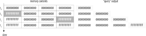
Reading a large chunk of memory is not an atomic operation. To construct a read-consistent image of a memory segment, you must either lock the segment for the duration of the query, or you must use a more complicated read consistency mechanism like the one the Oracle kernel uses for real tables. Otherwise, the output of the query may represent a system state that has never actually existed. Figure 8-1 illustrates the problem. A scan of a memory segment begins at time t 0 and concludes at time t 3. A dark box indicates a memory location whose contents are being changed at a given time. A lightly shaded box indicates the memory location whose contents are being copied to the output stream at a given time. Because reading a large chunk of memory is not an atomic operation, the output stream can contain a state that has never actually existed in memory at any time in the past.
The magnitude of the read consistency problem increases with
the execution duration of a snapshot. Imagine that fetching data for
2,000 Oracle sessions from a simple query upon V$SESSION motivates the sequence of events
depicted in Table
8-1. The query’s result set is not a snapshot, but a
collection of rows that all represent slightly different system
states smeared across the 0.40 seconds of the query’s total elapsed
time.
Time | Event |
0:00:00.00 | |
0:00:00.01 | First row of output is returned |
0:00:00.12 | Session number 1297 disconnects |
0:00:00.26 | The location in shared memory that contained information for session number 1297 no longer contains information about session 1297; hence, no data about session number 1297 (which was active at 10:00:00.00) is returned |
0:00:00.40 | Final row of output is returned |
Of course, the result of a query without a read-consistency guarantee is prone to be incorrect. The problem compounds when you attempt to include multiple data sources in your snapshots. Imagine that you have decided that each operational data snapshot you need contains data from each of the following Oracle fixed views:
V$BH |
V$DB_OBJECT_CACHE |
V$FILESTAT |
V$LATCH |
V$LIBRARYCACHE |
V$LOCK |
V$OPEN_CURSOR |
V$PARAMETER |
V$PROCESS |
V$ROLLSTAT |
V$ROWCACHE |
V$SESSION |
V$SESSION_EVENT |
V$SESSION_WAIT |
V$SESSTAT |
V$SQL |
V$SQLTEXT |
V$TIMER |
V$TRANSACTION |
V$WAITSTAT |
You would love to believe that all of the data collected
during a single snapshot actually represent a single instant in
time. However, it’s not true. For fixed views with only a small
number of relatively nonvolatile rows, this is not a big problem.
But for fixed views with thousands of rows, you can create strange
results with simple SELECT
statements. The problem is even worse if you have such a long list
of fixed views across which you wish to construct a snapshot. If
these were real Oracle tables, you would probably use the following
technique to force several queries to behave as though they were
participants in a single atomic event:
set transaction readonly; select * from v$bh; select * from v$db_object_cache; ... select * from v$waitstat; commit;
However, this strategy won’t work for V$ fixed views because they’re not real
tables. Regardless of how you collect the data for your snapshot,
the data will be slurred over the duration of the snapshot
collection query set. The time-state of the first row of the
V$BH query will differ from the
time-state of the last row of the V$WAITSTAT query by the accumulated
duration of these statements’ executions. The duration in this
example will likely be more than a whole second. No program can scan
gigabytes or even hundreds of megabytes of memory in a single atomic
operation.
It is very difficult to do time-based correlation among data sources, even for data collected within a single snapshot. The problem, of course, takes on even more complexity if you introduce operating system statistics into the collected data set.
Fixed View Reference
In spite of their deficiencies, Oracle’s fixed views provide value to the performance analyst in many situations. For this section, I describe a few Oracle fixed views that are important for you to understand in your role of performance analyst. All object descriptions shown were taken from an Oracle release 9.0.1.0.0 system.
V$SQL
Probably the most important fixed view for the
performance analyst is V$SQL.
This view shows several important attributes of the SQL statements
whose header information currently reside in the shared pool. The
columns in this view are as follows:
SQL> desc v$sql
Name Null? Type
-------------------------------------- -------- --------------------------
SQL_TEXT VARCHAR2(1000)
SHARABLE_MEM NUMBER
PERSISTENT_MEM NUMBER
RUNTIME_MEM NUMBER
SORTS NUMBER
LOADED_VERSIONS NUMBER
OPEN_VERSIONS NUMBER
USERS_OPENING NUMBER
EXECUTIONS NUMBER
USERS_EXECUTING NUMBER
LOADS NUMBER
FIRST_LOAD_TIME VARCHAR2(19)
INVALIDATIONS NUMBER
PARSE_CALLS NUMBER
DISK_READS NUMBER
BUFFER_GETS NUMBER
ROWS_PROCESSED NUMBER
COMMAND_TYPE NUMBER
OPTIMIZER_MODE VARCHAR2(10)
OPTIMIZER_COST NUMBER
PARSING_USER_ID NUMBER
PARSING_SCHEMA_ID NUMBER
KEPT_VERSIONS NUMBER
ADDRESS RAW(4)
TYPE_CHK_HEAP RAW(4)
HASH_VALUE NUMBER
PLAN_HASH_VALUE NUMBER
CHILD_NUMBER NUMBER
MODULE VARCHAR2(64)
MODULE_HASH NUMBER
ACTION VARCHAR2(64)
ACTION_HASH NUMBER
SERIALIZABLE_ABORTS NUMBER
OUTLINE_CATEGORY VARCHAR2(64)
CPU_TIME NUMBER
ELAPSED_TIME NUMBER
OUTLINE_SID NUMBER
CHILD_ADDRESS RAW(4)
SQLTYPE NUMBER
REMOTE VARCHAR2(1)
OBJECT_STATUS VARCHAR2(19)
LITERAL_HASH_VALUE NUMBER
LAST_LOAD_TIME VARCHAR2(19)
IS_OBSOLETE VARCHAR2(1)With V$SQL, you can
rank SQL statements in your system by the amount of work they do, or
by whatever measure of efficiency you like (see Section 8.3.3 later in
this chapter). By querying V$SQLTEXT_WITH_NEWLINES, you can see the
entire text of a SQL statement, not just the first 1,000 bytes that
are stored in V$SQL.SQL_TEXT:
select sql_text from v$sqltext_with_newlines where hash_value=:hv and address=:addr order by piece
You can even sense the presence of how distinct SQL texts might have been able to make more effective use of bind variables:
select count(*), min(hash_value), substr(sql_text,1,:len) from v$sql group by substr(sql_text,1,:len) having count(*)>=:threshold order by 1 desc, 3 asc
In this query, :len
specifies a SQL text prefix length that defines whether two distinct
statements are “similar” or not. For example, if :len=8, then the strings select s alary,... and select s .program,... are similar, because their
first eight characters are the same. Values like 32, 64, and 128
usually produce interesting results. The value of :threshold determines your threshold of
tolerance for similar statements in your library cache. You’ll
normally want to set :threshold
to at least three, because having only two similar SQL statements in
your library cache is not really a problem. If your system is
running amok in unshared SQL, then you’ll want to set :threshold to a larger value so that you
can focus on fixing a few unshared statements at a time.
V$SESS_IO
V$SESS_IO is a simple fixed view that allows you to measure the
logical and so-called physical I/O that has been generated for a
session:
SQL> desc v$sess_io
Name Null? Type
-------------------------------------- -------- --------------------------
SID NUMBER
BLOCK_GETS NUMBER
CONSISTENT_GETS NUMBER
PHYSICAL_READS NUMBER
BLOCK_CHANGES NUMBER
CONSISTENT_CHANGES NUMBERThe statistics in V$SESS_IO
map nicely to extended SQL trace statistics:
BLOCK_GETSThe equivalent of the
custatistic in raw trace data.CONSISTENT_GETSThe equivalent of the
crstatistic in raw trace data.PHYSICAL_READSThe equivalent of the
pstatistic in raw trace data.
The number of logical I/Os (LIOs) is the sum of the values of
BLOCK_GETS and CONSISTENT_GETS. When an Oracle session
consumes massive amounts of CPU capacity with only intermittent
executions of instrumented Oracle wait events, the session’s trace
will appear to “sit still.” With repeated executions of the
following query, you can observe whether a session that is running
but emitting no trace data is executing LIO calls:
select block_gets, consistent_gets from v$sess_io where sid=:sid
V$SYSSTAT
V$SYSSTAT is one of the first fixed views I remember using. Its
structure is simple:
SQL> desc v$sysstat
Name Null? Type
-------------------------------------- -------- --------------------------
STATISTIC# NUMBER
NAME VARCHAR2(64)
CLASS NUMBER
VALUE NUMBEREach row in V$SYSSTAT
contains an instance-wide statistic. Most statistics are tallies of
operations that have occurred since the most recent instance
startup. V$SYSSTAT rows are
subject to overflow errors.
The denormalized structure of V$SYSSTAT makes it easy to find out what
the system has done since the most recent instance startup, without
having to do a join. The following query executed in
Oracle9i displays roughly 250
statistics that describe what the entire instance has done over its
lifespan:
select name, value from v$sysstat order by 1
The following query lists the values of several statistics related to parsing:
select name, value from v$sysstat where name like 'parse%'
V$SESSTAT
As I described in Chapter 3, the system-wide scope
is probably the incorrect action scope for your diagnostic data
collection. V$SESSTAT contains
the same statistics as V$SYSSTAT,
except at the session level:
SQL> desc v$sesstat
Name Null? Type
-------------------------------------- -------- --------------------------
SID NUMBER
STATISTIC# NUMBER
VALUE NUMBEREach row in V$SESSTAT
contains a tally of how many times a statistic has been incremented
since the creation of a specified session.
V$SESSTAT is not
denormalized like V$SYSSTAT, so
finding a statistic by name requires a join with V$STATNAME. The following query lists all
the statistics that have aggregated for a session since its
birth:
select name, value from v$statname n, v$sesstat s where sid=:sid and n.statistic#=s.statistic# and s.value>0 order by 2
The following query lists the approximate number of centiseconds’ worth of CPU capacity consumed by a given session:
select name, value from v$statname n, v$sesstat s where sid=:sid and n.statistic#=s.statistic# and n.name='CPU used by this session'
V$SYSTEM_EVENT
The V$SYSTEM_EVENT
fixed view records aggregated statistics about instrumented code
paths that the Oracle kernel has executed since its most recent
instance startup:
SQL> desc v$system_event
Name Null? Type
-------------------------------------- -------- --------------------------
EVENT VARCHAR2(64)
TOTAL_WAITS NUMBER
TOTAL_TIMEOUTS NUMBER
TIME_WAITED NUMBER
AVERAGE_WAIT NUMBER
TIME_WAITED_MICRO NUMBEREach row in V$SYSTEM_EVENT
contains information about the calls of a given event for the
lifespan of the instance.
Tip
You might notice that there is no MAX_WAIT column in V$SYSTEM_EVENT. You can add this useful
column to the definition of V$SYSTEM_EVENT, if you like, by
following the instructions presented in [Lewis (2001b)
577-581].
On Oracle7 and Oracle8i kernels, you can obtain resource consumption statistics about everything but CPU consumption with following query:
select event, total_waits, time_waited/100 t from v$system_event order by 3 desc
With Oracle9i kernels, you can obtain the same statistics displayed with microsecond precision by using the following query:
select event, total_waits, time_waited_micro/1000000 t from v$system_event order by t desc
V$SESSION_EVENT
Once again, the system-wide scope is often the
incorrect scope for diagnostic data collection. V$SESSION_EVENT provides the ability to
collect properly session-scoped diagnostic data for Oracle kernel
code paths:
SQL> desc v$session_event
Name Null? Type
-------------------------------------- -------- --------------------------
SID NUMBER
EVENT VARCHAR2(64)
TOTAL_WAITS NUMBER
TOTAL_TIMEOUTS NUMBER
TIME_WAITED NUMBER
AVERAGE_WAIT NUMBER
MAX_WAIT NUMBER
TIME_WAITED_MICRO NUMBEREach row in V$SESSION_EVENT
contains information about the executions of a given segment of
Oracle kernel code (a “wait event”) for a given session since its
birth. Thus, the information in V$SESSION_EVENT is an aggregation of the
data that appears in extended SQL trace output:
EVENTThe name of an Oracle wait event. Note that each
EVENTvalue corresponds to anamvalue in theWAITlines of Oracle’s extended SQL trace data.TOTAL_WAITSThe number of
WAITlines withnam='x', where x is the value of the row’sEVENT.TIME_WAITEDThe sum of the
elavalues for allWAITlines withnam='x', where x is the value of the row’sEVENT.
The V$SESSION_EVENT fixed
view contains no record of a session’s CPU capacity consumption. You
have to go to V$SESSTAT for
that.
The following query will display information about the wait events that a given Oracle8i session has executed over its lifespan:
select event, total_waits, time_waited/100 t from v$session_event where sid=:sid order by t desc
The following query will display information about the wait events that a given Oracle9i session has executed over its lifespan:
select event, total_waits, time_waited_micro/1000000 t from v$session_event where sid=:sid order by t desc
V$SESSION_WAIT
Ask people what the “wait interface” is, and most will
probably mention V$SESSION_WAIT.
Unlike the V$SYSTEM_EVENT and
V$SESSION_EVENT fixed views, V$SESSION_WAIT does not contain an
aggregation of historical events. Instead, it provides a view into
what a specified session is doing right
now:
SQL> desc v$session_wait
Name Null? Type
-------------------------------------- -------- --------------------------
SID NUMBER
SEQ# NUMBER
EVENT VARCHAR2(64)
P1TEXT VARCHAR2(64)
P1 NUMBER
P1RAW RAW(4)
P2TEXT VARCHAR2(64)
P2 NUMBER
P2RAW RAW(4)
P3TEXT VARCHAR2(64)
P3 NUMBER
P3RAW RAW(4)
WAIT_TIME NUMBER
SECONDS_IN_WAIT NUMBER
STATE VARCHAR2(19)Each row in V$SESSION_WAIT
contains information about a session’s present state. The statistics
revealed by V$SESSION_WAIT
include:
SEQ#Each time an event completes, the Oracle kernel increments this sequence number.
WAIT_TIMEAt the beginning of an instrumented wait event, the Oracle kernel sets the value of
WAIT_TIMEto zero. The value remains zero until the wait event is complete, when the kernel sets its value to one of those shown in Table 8-2. Note that the unit of measure is the centisecond, even in Oracle9i. There is noWAIT_TIME_MICROcolumn at least through release 9.2.0.2.1, although the value ofWAIT_TIMEis derived from a microsecond value in its underlyingX$view.SECONDS_IN_WAITAt the beginning of an instrumented wait event, the Oracle kernel sets the value of
SECONDS_IN_WAITto zero. The session itself never updates the value again until the next instrumented wait event, whereupon the session resets the value back to zero again. The value ofSECONDS_IN_WAITis incremented by 3 approximately every three seconds by the log writer (LGWR) process. Note that the unit of measure is seconds, not centiseconds or microseconds.Events that “time out” complicate matters somewhat. For example, an
enqueuewait event times out roughly every two seconds, even for enqueue waits that last considerably longer. Upon each timeout, the Oracle kernel incrementsSEQ#, but it does not reset the value ofSECONDS_IN_WAIT.STATEAt the beginning of an instrumented wait event, the value of
STATEbecomesWAITING. The value remainsWAITINGuntil the wait event is complete, when the kernel sets its value to one of the values described in Table 8-2.
STATE | WAIT_TIME | Implication |
| | The value of |
| | The wait event has completed, but it began and
ended within the same |
| 0 | The wait event is in process, pending completion. |
| t ≥ 0 | The wait event has completed, and it consumed t = t 1 - t 0 centiseconds of elapsed execution time (Chapter 7). |
The following query will display information about the wait events that are presently executing on a given Oracle system:
select sid, event, wait_time/100 t, seconds_in_wait w, state from v$session_wait order by 1
The following query will show a histogram of which activity your system’s sessions are doing right now:
select event, count(*) from v$session_wait where state='WAITING' group by event order by 2 desc
Warning
Don’t write V$SESSION_WAIT queries with WAIT_TIME=0 in your where clause if what you really mean is
STATE='WAITING‘. Some analysts
got into the habit of assuming that the predicates WAIT_TIME=0 and STATE='WAITING' are equivalent, because
in Oracle7 and Oracle8i
kernels, they were. However, in Oracle9i kernels, the two predicates are not
equivalent.
Oracle9i kernels
compute WAIT_TIME as round(x$ksusecst.ksusstim/10000), but
the STATE value is a DECODE of the
un-rounded value of KSUSSTIM. Therefore, WAIT_TIME can appear to be zero when its
base data value is actually not. Hence, Oracle9i kernels produce situations in which
WAIT_TIME is zero, but STATE is something other than WAITING.
Useful Fixed View Queries
Almost every database administrator has a tool kit of
V$ queries that she uses to help
with database performance analysis work. This section discusses some
of my favorites and I’m sure some of yours as well. Be prepared
though. Chances are good that some of the reports you count on for
information today are feeding you misleading data. Practically every
V$ query you can run is susceptible
to one or more serious interpretation fallacies. This section
illustrates several.
Tom Kyte’s Test Harness
One of my favorite fixed view-based tools ever is Tom Kyte’s test harness that allows an application developer to compare the performance of two competing application development approaches. You can see a complete description online at http://asktom.oracle.com/~tkyte/runstats.html. This URL contains instructions about how to use the simple harness, including an example of using the harness to demonstrate the horrifyingly bad scalability of applications that do not use bind variables (http://asktom.oracle.com/pls/ask/f?p=4950:8:::::F4950_P8_DISPLAYID:2444907911913).
Tom’s test harness is especially valuable for developers of Oracle applications to use early in their SQL development cycles. Developers usually write code that users will later execute on a busy system. However, the systems on which developers write that code are usually not busy—at least not in the same way that their users’ systems are. Tom’s test harness measures an application’s use of the Oracle resources that scale the worst (including, perhaps most notably, Oracle latches). The results are simple to interpret. The fewer serialized resources that an approach requires, the better you can expect it to scale when it becomes a part of your production workload. The best thing about Tom’s harness is that it’s so easy to use that developers actually will use it. Once developers start thinking in the terms of the resource consumption data that the harness provides, they write more scalable code.
Finding a Fixed View Definition
It can be difficult to find the information you need
about a V$ fixed view from
publications about Oracle. Sometimes the information you want is
simply not published. Other times you find the information that you
think you’re looking for, but it’s just plain wrong. Publications
about Oracle are particularly unreliable in areas of the Oracle
kernel that evolve quickly. Fortunately, the kernel is somewhat
self-documenting in the domain of fixed views. One secret lies
within knowing how to use V$FIXED_VIEW_DEFINITION. The hardest part
is knowing its name:
SQL> desc v$fixed_view_definition
Name Null? Type
-------------------------------------- -------- --------------------------
VIEW_NAME VARCHAR2(30)
VIEW_DEFINITION VARCHAR2(4000)V$FIXED_VIEW_DEFINITION is
the means through which I learned, for example, the detailed
definitions of the STATE and
WAIT_TIME columns of V$SESSION_WAIT. You can reproduce the
result in just a few simple steps. Begin by executing the following
query to return the definition of the V$SESSION_WAIT view:
SQL>select * from v$fixed_view_definition2where view_name='V$SESSION_WAIT';VIEW_NAME ------------------------------ VIEW_DEFINITION --------------------------------------------------------------------------- V$SESSION_WAIT select sid,seq#,event,p1text,p1,p1raw,p2text,p2,p2raw,p3text, p3,p3raw,wait _time,seconds_in_wait,statefrom gv$session_waitwhere inst_id = USERENV('I nstance')
Notice, by the way, that the VIEW_NAME value for this view is stored
using uppercase letters. So now you know that V$SESSION_WAIT is simply a projection of
GV$SESSION_WAIT. That doesn’t
tell you very much yet, however. The next step is to figure out the
definition of GV$SESSION_WAIT:
SQL>desc gv$session_waitName Null? Type -------------------------------------- -------- -------------------------- INST_ID NUMBER SID NUMBER SEQ# NUMBER EVENT VARCHAR2(64) P1TEXT VARCHAR2(64) P1 NUMBER P1RAW RAW(4) P2TEXT VARCHAR2(64) P2 NUMBER P2RAW RAW(4) P3TEXT VARCHAR2(64) P3 NUMBER P3RAW RAW(4) WAIT_TIME NUMBER SECONDS_IN_WAIT NUMBER STATE VARCHAR2(19) SQL>select * from v$fixed_view_definition2where view_name='GV$SESSION_WAIT';VIEW_NAME ------------------------------ VIEW_DEFINITION --------------------------------------------------------------------------- GV$SESSION_WAIT select s.inst_id,s.indx,s.ksussseq,e.kslednam, e.ksledp1,s.ksussp1,s.ksussp 1r,e.ksledp2, s.ksussp2,s.ksussp2r,e.ksledp3,s.ksussp3,s.ksussp3r,round(s.ksusstim / 10000), s.ksusewtm,decode(s.ksusstim, 0, 'WAITING', -2, 'WAITEDUNKNOWN TIME', -1, 'WAITED SHORT TIME', 'WAITED KNOWN TIME')from x$ksus ecst s, x$ksled e where bitand(s.ksspaflg,1)!=0 and bitand(s.ksuseflg,1)!=0 and s.ksussseq!=0 and s.ksussopc=e.indx
Voilà! Here you can see the rounding operation used to compute
WAIT_TIME. From what you see
here, you can also determine the unit of measure in which this thing
called X$KSUSECST.KSUSSTIM is
expressed. We know that WAIT_TIME
is reported in centiseconds, and we know that the Oracle kernel
divides this value by 104 to produce a
centisecond value. Therefore, there are 10
k KSUSSTIM units in one second, where
10 k
/104 =
102. Hence, there are
106 KSUSSTIM units in a second. In other
words, the Oracle kernel computes the wait time in microseconds, but
the public API (V$SESSION_WAIT)
provides it in centiseconds.
Finding Inefficient SQL
Jeff Holt’s htopsql.sql script,
shown in Example 8-2,
is what http://www.hotsos.com staff use when
we wish to get a fast overview of which SQL statements presently in
the library cache have contributed the most to recent workload. The
query has no direct relationship to response time, but there is a
strong correlation between a query’s LIO count and the total
execution time for most SQL statements. The new columns CPU_TIME and ELAPSED_TIME, available in
Oracle9i, reveal in V$SQL some of the data previously
available only in SQL trace data.
rem $Header: /usr/local/hostos/RCS/htopsql.sql,v 1.6 2001/11/19 22:31:35 rem Author: [email protected] rem Copyright (c) 1999 by Hotsos Enterprises, Ltd. All rights reserved. rem Usage: This script shows inefficient SQL by computing the ratio rem of logical_reads to rows_processed. The user will have rem to press return to see the first page. The user should rem be able to see the really bad stuff on the first page and rem therefore should press ^C and then press [Return] when the rem first page is completely displayed. rem SQL hash values are really statement identifiers. These rem identifiers are used as input to a hashing function to rem determine if a statement is in the shared pool. rem This script shows only statement identifiers. Use hsqltxt.sql rem to display the text of interesting statements. rem Notes: This will return data for select,insert,update, and delete rem statements. We don't return rows for PL/SQL blocks because rem their reads are counted in their underlying SQL statements. rem There is value in knowing the PL/SQL routine that executes rem an inefficient statement but it's only important once you rem know what's wrong with the statment. col stmtid heading 'Stmt Id' format 9999999999 col dr heading 'PIO blks' format 999,999,999 col bg heading 'LIOs' format 999,999,999 col sr heading 'Sorts' format 999,999 col exe heading 'Runs' format 999,999,999 col rp heading 'Rows' format 9,999,999,999 col rpr heading 'LIOs|per Row' format 999,999,999 col rpe heading 'LIOs|per Run' format 999,999,999 set termout on set pause on set pagesize 30 set pause 'More: ' set linesize 95 select hash_value stmtid ,sum(disk_reads) dr ,sum(buffer_gets) bg ,sum(rows_processed) rp ,sum(buffer_gets)/greatest(sum(rows_processed),1) rpr ,sum(executions) exe ,sum(buffer_gets)/greatest(sum(executions),1) rpe from v$sql where command_type in ( 2,3,6,7 ) group by hash_value order by 5 desc / set pause off
The query sorts its output by the number of LIO calls executed per row returned. This is a rough measure of statement efficiency. For example, the following output should bring to mind the question, “Why should an application require more than 174 million memory accesses to compute 5 rows?”
SQL> @htopsql
More:
LIOs LIOs
Stmt Id PIO blks LIOs Rows per Row Runs per Run
---------- ----------- ------------ ---- ------------ ---------- ----------
2503207570 39,736 871,467,231 5 174,293,446 138 6,314,980
1647785011 10,287,310 337,616,703 3 112,538,901 7,730,556 44
4085942203 45,748 257,887,860 8 32,235,983 138 1,868,753
3955802477 10,201 257,887,221 8 32,235,903 138 1,868,748
1647618855 53,136 5,625,843 0 5,625,843 128,868 44
3368205675 35,666 3,534,374 0 3,534,374 1 3,534,374
3722360728 54,348 722,866 1 722,866 1 722,866
497954690 54,332 722,779 0 722,779 1 722,779
90462217 361,189 4,050,206 8 506,276 137 29,564
299369270 1,268 382,211 0 382,211 42,378 9
...The output shown here was used in 1999 to identify a single SQL statement that was consuming almost 50% of the total daily CPU capacity of an online system. However, as with any ratio, the LIOs per row definition of statement efficiency can motivate false conclusions. For example, consider a SQL statement like this one:
select cust, sum(bal) from colossal_order_history_table where cust_id=:id group by cust
This query may legitimately visit a very large number of
Oracle blocks (even using a primary key index on CUST_ID), but it will at most return only
one row. An htopsql.sql report would thus imply
that this query is inefficient, when in fact this might be a false
negative implication.
Many analysts use a query like
htopsql.sql as the beginning step in each of
their performance improvement projects. However, basing a
performance improvement method upon any report upon V$SQL suffers from deficiencies induced by
time scope and program scope errors. Like most information you learn
from V$ fixed views, it is
difficult to exercise control over the time scope and program scope
of data obtained from V$SQL. For
example, consider the following situations:
The SQL statement that most needs your attention is one that has not been run since last month’s month-end close. The statement is no longer in the library cache, so it will not be revealed in today’s
V$SQLreport.The SQL statement that appears “most inefficient” is an element of an interface upload program that your company will never run again.
The SQL statement that appears “most inefficient” is one that runs from midnight to 3:00 a.m. Since its window of permissible execution time extends until 6:00 a.m., and since all the nightly batch work finishes long before that deadline, nobody cares that the inefficient SQL statement is slow.
The SQL statement whose performance is most hurting the business’s ability to improve net profit, cash flow, and return on investment is not listed near the top of any of your
V$SQLreports. Its ranking is mediocre because none of its statistics is particularly remarkable, but from the business’s perspective, this is clearly the statement that is most hurting the system’s economic value.
Without obtaining information from the
business, there is no way to know whether the
performance of a SQL statement that rises to the top of the report
is actually even critical to the business. I believe that V$SQL is any performance analyst’s most
valuable V$ fixed view in the
database. However, the power of using V$SQL is far less than the power of a
performance improvement project that follows Method R.
Finding Where a Session Is Stuck
From time to time, we all get that call. It’s Nancy on the phone, and her session is “stuck.” She’s asked her colleagues already if the system is down, and everyone else around her seems to be working fine. Perhaps the reason Nancy’s calling is because in last week’s brown-bag lunch event,[1] you explained to your users why they should not reboot their personal computer when this kind of thing happens. If you know how to find Nancy’s session ID (Chapter 6), then it is easy to determine what’s going on with her session. Imagine that we had found out that Nancy’s session ID is 42. Then you use the following query to determine why she’s stuck:
SQL>col sid format 999990SQL>col seq# format 999,990SQL>col event format a26SQL>select sid, seq#, event, state, seconds_in_wait seconds2from v$session_wait3where sid=42SID SEQ# EVENT STATE SECONDS ------- -------- -------------------------- ------------------- ---------- 42 29,786 db file sequential read WAITED SHORT TIME 174
Does this mean that Nancy’s session is stuck waiting for I/O? No; actually this query indicates the contrary. The most recent wait event that Nancy’s Oracle kernel process executed was in fact a file read operation, but the operation completed approximately 174 seconds ago (plus or minus roughly 3 seconds). Furthermore, the operation completed in less than one unit of Oracle timer resolution. (On an Oracle8i system, this means that the elapsed time of the read operation was less than 0.01 seconds.) So what is Nancy’s session waiting on?
The answer is that her session (really, her Oracle kernel
process) is either working its brains out consuming CPU capacity, or
her session is waiting its turn in the ready to run queue for its next
opportunity to work its brains out consuming CPU capacity. You can
watch what the session is doing by issuing successive queries of
V$SESS_IO:
SQL>col block_gets format 999,999,999,990SQL>col consistent_gets format 999,999,999,990SQL>select to_char(sysdate, 'hh:mi:ss') "TIME",2block_gets, consistent_gets3from v$sess_io where sid=42;TIME BLOCK_GETS CONSISTENT_GETS -------- ---------------- ---------------- 05:20:27 2,224 22,647,561 SQL>/TIME BLOCK_GETS CONSISTENT_GETS -------- ---------------- ---------------- 05:20:44 2,296 23,382,994
By incorporating a timestamp into your query, you can get a
feel for the rate at which your Oracle system can process LIO calls.
The system shown here processed 735,505 LIO calls in about 17
seconds, which yields a rate of 43,265 LIOs per second. With this
information, you can begin to appreciate what Nancy is going
through. The more than 22,000,000 LIOs executed by her program when
you first began looking at it had already consumed almost nine
minutes of execution time. It’s time now for you to find out what
SQL Nancy’s program is running so that you can get it fixed. You can
do that job by joining V$OPEN_CURSOR and V$SQL. I’d rather have extended SQL trace
data for Nancy’s program if I could get it, but if you don’t have
that luxury, smart use of Oracle’s fixed views can help you find the
problem.
Finding Where a System Is Stuck
Sometimes the phone rings, and before Nancy finishes describing her problem, you notice another incoming call on line two. Then within two minutes, you’ve heard complaints from four users, and you have seven new voicemails containing ones you haven’t heard yet. What should you do? If your system permits the execution of a query, here’s the one I’d suggest that you run:
SQL>break on reportSQL>compute sum of sessions on reportSQL>select event, count(*) sessions from v$session_wait2where state='WAITING'3group by event4order by 2 desc;EVENT SESSIONS ---------------------------------------------------------------- ---------- SQL*Net message from client 211 log file switch (archiving needed) 187 db file sequential read 27 db file scattered read 9 rdbms ipc message 4 smon timer 1 pmon timer 1 ---------- sum 440
The report shown here depicts 440 connected sessions. At the
time of the query, over 200 of the Oracle kernel processes are
blocked on a read of the SQL*Net socket while their end-user
applications execute code path between database calls. Many of these
211 processes are probably sitting idle while their users use
non-Oracle applications, talk with colleagues, or attend to one or
more of our species’ many physiological needs. More disturbing is
that 187 sessions are blocked waiting for log file switch
(archiving needed). This message indicates that the Oracle
ARCH process is not able to keep pace with the generation of online
redo.
A few other users on the system are actually getting work done
(36 are engaged in reading database files), but as each user
attempts to execute a database COMMIT call, she’ll get caught waiting for
a log file switch (archiving
needed) event. The longer the problem goes uncorrected,
the more users will get stuck waiting for the event. On the system
where this output was obtained, the database administrator had
neglected to anticipate that on this particular day, the ARCH process’s destination file system
would fill.
Approximating a Session’s Resource Profile
The program vprof, shown in Example 8-3, is something that I cobbled together to collect Oracle timing data for a specified Oracle session for a specified time interval. I designed vprof not for production use (I don’t consider it worthy for production use), but to illustrate some of the complexities of trying to use SQL upon fixed views to perform well-scoped diagnostic data collection. I find vprof to be useful in educational environments to help explain points including:
The union of data from
V$SESSTATandV$SESSION_EVENTapproximately accounts for the total response time of a user action.Attempts to obtain user action timing data from Oracle
V$fixed views are plagued by difficult time scope challenges.Diagnosing the performance problem of a targeted user action is a much bigger job than just creating the action’s resource profile.
#!/usr/bin/perl # $Header: /home/cvs/cvm-book1/sqltrace/vproP.pl,v 1.8 2003/04/08 14:27:30 # Cary Millsap ([email protected]) # Copyright (c) 2003 by Hotsos Enterprises, Ltd. All rights reserved. use strict; use warnings; use Getopt::Long; use DBI; use Time::HiRes qw(gettimeofday); use Date::Format qw(time2str); sub nvl($;$) { my $value = shift; my $default = shift || 0; return $value ? $value : $default; } # fetch command-line options my %opt = ( service => "", username => "/", password => "", debug => 0, ); GetOptions( "service=s" => $opt{service}, "username=s" => $opt{username}, "password=s" => $opt{password}, "debug" => $opt{debug}, ); # fetch sid from command line my $usage = "Usage: $0 [options] sid "; my $sid = shift or die $usage; # connect to Oracle and prepare snapshot SQL my %attr = (RaiseError => 1, AutoCommit => 0); my $dbh = DBI->connect( "dbi:Oracle:$opt{service}", $opt{username}, $opt{password}, \%attr ); my $sth = $dbh->prepare(<<'END OF SQL', {ora_check_sql => 0}); select 'CPU service' ACTIVITY, value TIME, ( select value from v$sesstat s, v$statname n where sid = ? and n.statistic# = s.statistic# and n.name = 'user calls' ) CALLS from v$sesstat s, v$statname n where sid = ? and n.statistic# = s.statistic# and n.name = 'CPU used by this session' union select e.event ACTIVITY, e.time_waited TIME, e.total_waits CALLS from v$session_event e where sid = ? END OF SQL # wait for signal and collect t0 consumption snapshot print "Press <Enter> to mark time t0: "; <>; my ($sec0, $msec0) = gettimeofday; $sth->execute($sid, $sid, $sid); my $h0 = $sth->fetchall_hashref("ACTIVITY"); # wait for signal and collect t1 consumption snapshot print "Press <Enter> to mark time t1: "; <>; my ($sec1, $msec1) = gettimeofday; $sth->execute($sid, $sid, $sid); my $h1 = $sth->fetchall_hashref("ACTIVITY"); # construct profile table my %prof; for my $k (keys %$h1) { my $calls = $h1->{$k}->{CALLS} - nvl($h0->{$k}->{CALLS}) or next; $prof{$k}->{CALLS} = $calls; $prof{$k}->{TIME} = ($h1->{$k}->{TIME} - nvl($h0->{$k}->{TIME})) / 100; } # compute unaccounted-for duration my $interval = ($sec1 - $sec0) + ($msec1 - $msec0)/1E6; my $accounted = 0; $accounted += $prof{$_}->{TIME} for keys %prof; $prof{"unaccounted-for"} = { ACTIVITY => "unaccounted-for", TIME => $interval - $accounted, CALLS => 1, }; # print debugging output if requested if ($opt{debug}) { use Data::Dumper; printf "t0 snapshot: %s ", Dumper($h0); printf "t1 snapshot: %s ", Dumper($h1); print " "; } # print the resource profile print " Resource Profile for Session $sid "; printf "%24s = %s.%06d ", "t0", time2str("%T", $sec0), $msec0; printf "%24s = %s.%06d ", "t1", time2str("%T", $sec1), $msec1; printf "%24s = %15.6fs ", "interval duration", $interval; printf "%24s = %15.6fs ", "accounted-for duration", $accounted; print " "; my ($c1, $c2, $c4, $c5) = (32, 10, 10, 11); my ($c23) = ($c2+1+7+1); printf "%-${c1}s %${c23}s %${c4}s %${c5}s ", "Response Time Component", "Duration (seconds)", "Calls", "Dur/Call"; printf "%-${c1}s %${c23}s %${c4}s %${c5}s ", "-"x$c1, "-"x$c23, "-"x$c4, "-"x$c5; for my $k (sort { $prof{$b}->{TIME} <=> $prof{$a}->{TIME} } keys %prof) { printf "%-${c1}s ", $k; printf "%${c2}.2f ", $prof{$k}->{TIME}; printf "%7.1f%% ", $prof{$k}->{TIME}/$interval*100; printf "%${c4}d ", $prof{$k}->{CALLS}; printf "%${c5}.6f ", ($prof{$k}->{CALLS} ? $prof{$k}->{TIME}/$prof{$k}->{CALLS} : 0); } printf "%-${c1}s %${c23}s %${c4}s %${c5}s ", "-"x$c1, "-"x$c23, "-"x$c4, "-"x$c5; printf "%-${c1}s %${c2}.2f %7.1f%% ", "Total", $interval, $interval/$interval*100; # wrap up $dbh->disconnect; _ _END_ _ =head1 NAME vprof - create an approximate resource profile for a session =head1 SYNOPSIS vprof [--service=I<h>] [--username=I<u>] [--password=I<p>] [--debug=I<d>] I<session-id> =head1 DESCRIPTION B<vprof> uses queries from B<V$SESSTAT> and B<V$SESSION_EVENT> to construct an approximate resource profile for the Oracle session whose B<V$SESSION.SID> value is given by I<session-id>. The time scope of the observation interval is defined interactively by the user's response to the prompts to mark the times I<t0> and I<t1>, where I<t0> is the observation interval start time, and I<t1> is the observation interval end time. =head2 Options =over 4 =item B<--service=>I<h> The name of the Oracle service to which B<vprof> will connect. The default value is "" (the empty string), which will cause B<vprof> to connect using, for example, the default Oracle TNS alias. =item B<--username=>I<u> The name of the Oracle schema to which B<vprof> will connect. The default value is "/". =item B<--password=>I<p> The Oracle password that B<vprof> will use to connect. The default value is "" (the empty string). =item B<--debug=>I<d> When set to 1, B<vprof> dumps its internal data structures in addition to its normal output. The default value is 0. =back =head1 EXAMPLES Use of B<vprof> will resemble something like the following case in which I used B<vprof> to report on statistics generated by B<vprof>'s own Oracle connection: $ vprof --username=system --password=manager 8 Press <Enter> to mark time t0: Press <Enter> to mark time t1: Resource Profile for Session 8 t0 = 14:59:12.596000 t1 = 14:59:14.349000 interval duration = 1.753000s accounted-for duration = 1.670000s Response Time Component Duration (seconds) Calls Dur/Call ----------------------------- -------------------- --------- ---------- SQL*Net message from client 1.38 78.7% 1 1.380000 CPU service 0.29 16.5% 1 0.290000 unaccounted-for 0.08 4.7% 1 0.083000 SQL*Net message to client 0.00 0.0% 1 0.000000 ----------------------------- -------------------- --------- ---------- Total 1.75 100.0% =head1 AUTHOR Cary Millsap ([email protected]) =head1 BUGS B<vprof> suffers from several severe limitations, including: =over 2 =item - If a wait event is pending at time I<t0>, then the profile will contain excess time, which will manifest as negative "unaccounted-for" time. This situation happens frequently for the event 'SQL*Net message from client'. This is the wait event whose execution is pending while an application user is idle. =item - If a wait event is pending at time I<t1>, then the profile will be absent some missing time, which will manifest as positive "unaccounted-for" time. This situation is likely to happen if you choose time I<t1> to occur during a long-running program. =item - The limitations listed above can combine to offset each other, on occasion resulting in small "unaccounted-for" duration. This produces a false positive indication that everything is alright when actually there are two problems. =item - If the specified sid does not exist at time I<t0>, then the program will return a profile filled with unaccounted-for time. =item - If a session with the specified sid terminates between time I<t0> and I<t1>, then the resulting resource profile will contain only unaccounted-for time. ...Unless a new session with the specified B<sid> (but of course a different B<serial#>) is created before I<t1>. In this case, the output will look appropriate but be completely erroneous. =back =head1 COPYRIGHT Copyright (c) 2000-2003 by Hotsos Enterprises, Ltd. All rights reserved.
The output of vprof looks
like this for a session on my system with V$SESSION.SID=8:
$ perl vprof.pl --username=system --password=manager 8
Press <Enter> to mark time t0: [RETURN]
Press <Enter> to mark time t1: [RETURN]
Resource Profile for Session 8
t0 = 09:08:00.823000
t1 = 09:08:01.103000
interval duration = 0.280000s
accounted-for duration = 0.280000s
Response Time Component Duration (seconds) Calls Dur/Call
-------------------------------- -------------------- ----------- ---------
CPU service 0.27 96.4% 1 0.270000
SQL*Net message from client 0.01 3.6% 1 0.010000
unaccounted-for 0.00 0.0% 1 0.000000
SQL*Net message to client 0.00 0.0% 1 0.000000
-------------------------------- -------------------- ----------- ---------
Total 0.28 100.0%The chief benefit of vprof is how it puts CPU service, unaccounted-for time, and the actual Oracle wait events on an equal footing to create a real resource profile. The output of vprof gets really interesting when you experiment with the timing of the two interactive inputs. For example, if you mark the time t 0 several seconds before the session under diagnosis does anything, then vprof will produce a large negative unaccounted-for duration, as follows:
$ perl vprof.pl --username=system --password=manager 58
Press <Enter> to mark time t0: [RETURN]
Press <Enter> to mark time t1: [RETURN]
Resource Profile for Session 58
t0 = 23:48:18.072254
t1 = 23:49:09.992339
interval duration = 51.920085s
accounted-for duration = 86.990000s
Response Time Component Duration (seconds) Calls Dur/Call
-------------------------------- ------------------- ---------- -----------
SQL*Net message from client 54.04 104.1% 2 27.020000
CPU service 31.98 61.6% 3 10.660000
db file sequential read 0.93 1.8% 29181 0.000032
async disk IO 0.03 0.1% 6954 0.000004
direct path read 0.01 0.0% 1228 0.000008
SQL*Net message to client 0.00 0.0% 2 0.000000
db file scattered read 0.00 0.0% 4 0.000000
direct path write 0.00 0.0% 2 0.000000
unaccounted-for -35.07 -67.5% 1 -35.069915
-------------------------------- ------------------- ---------- -----------
Total 51.92 100.0% At the time t
0, a long SQL*Net
message from client event was in-process, so none of its
total duration had yet been tallied to V$SESSION_EVENT. By the arrival of time
t 1, the
entire long SQL*Net message from
client event had tallied to V$SESSION_EVENT, but part of that event
duration occurred prior to the beginning of the observation
interval. The vprof program
computed the interval duration correctly as t 1 - t 0, but the total
Oracle event time accounted for between times t 1 and t 0 exceeded the
quantity t
1 - t
0, so vprof introduced a negative unaccounted-for pseudo-event to true up
the profile.
This is a nice example of collection
error that can taint your diagnostic data (see Chapter 6 for more on the topic of
collection error). If you were to improve the production-worthiness
of vprof, you could check
V$SESSION_WAIT for an in-process
event execution at t
0 and then correct for it based on what you
found. This is the kind of thing we did in the year 2000 for our big
V$ data analysis project. It was
after figuring out how to correct several problems like this that we
discovered all the other limitations described earlier in this
chapter and decided to cut our losses on the project. For example,
what if enqueue waits had shown
up at the top of your resource profile? How would you go about
determining which lock it was that your program under diagnosis had
waited on (past tense) when it was running?
Performing further diagnosis of such a problem without properly
time- and action-scoped data is a non-deterministic process that can
easily result in one of the project catastrophes described in Chapter 1.
Viewing Waits System-Wide
One of the most popular reports on system performance executed since the mid-1990s is probably the system-wide events report. Just about the simplest decent version of the report looks something like this:
SQL>col event format a46SQL>col seconds format 999,999,990.00SQL>col calls format 999,999,990SQL>select event, time_waited/100 seconds, total_waits calls2from v$system_event3order by 2 desc;EVENT SECONDS CALLS ---------------------------------------------- --------------- ------------ rdbms ipc message 13,841,814.91 3,671,093 pmon timer 3,652,242.44 1,305,093 smon timer 3,526,140.14 12,182 SQL*Net message from client 20,754.41 12,627 control file parallel write 2,153.49 1,218,538 db file sequential read 91.61 547,488 log file parallel write 55.66 23,726 db file scattered read 26.26 235,882 control file sequential read 8.12 365,643 control file heartbeat 3.99 1 latch activity 2.93 30 buffer busy waits 1.41 72 resmgr:waiting in end wait 0.93 44 latch free 0.80 39 resmgr:waiting in check 0.53 36 log file sync 0.28 19 process startup 0.22 6 rdbms ipc reply 0.14 9 db file parallel read 0.11 4 async disk IO 0.10 19,116 db file parallel write 0.09 24,420 SQL*Net more data to client 0.09 2,014 resmgr:waiting in check2 0.06 2 SQL*Net message to client 0.06 12,635 direct path read 0.05 5,014 log file sequential read 0.03 4 refresh controlfile command 0.00 1 log file single write 0.00 4 SQL*Net break/reset to client 0.00 23 direct path write 0.00 10 30 rows selected.
This type of report is supposed to help the performance analyst instantly determine the nature of a “system’s” performance problem. However, the report has many problems living up to that job description. Reports like this can help you solve some types of performance problems, but they fail to help you solve many of the problems I’ve illustrated throughout this book, such as:
Problems with user actions whose performance characteristics do not resemble the system-wide average performance characteristics. You cannot extrapolate detail from an aggregate. Not realizing this can lead to accidental performance degradation for important user actions for the reasons described in Chapter 4.
Problems with user actions whose performance problems can be diagnosed quickly by observing
SQL*Net message from clientdurations that should be counted as user action response time. Does theSQL*Net message from clientduration shown in aV$SYSTEM_EVENTreport indicate a network I/O inefficiency, or that an application is issuing an excessive number of database calls? You simply can’t tell fromV$SYSTEM_EVENTdata. Big numbers might indicate problems like these. And big numbers might indicate simply that users spend a lot of time connected but not doing anything productive.
Relying on V$SYSTEM_EVENT
reports thus returns me to the topic I addressed in Chapter 3 about whether it makes
sense to use different methods for different problems. Using
different methods to diagnose different problem types presupposes
that you can guess what the problem is before you begin your
diagnosis. This is the method deficiency that causes many of the
project catastrophes that I describe in Chapter 1.
The following sections illustrate some of the reasons why
V$SYSTEM_EVENT reports fail to
help you solve certain performance problem types.
The “idle events” problem
From looking at the system-wide events report shown
previously, a naïve analyst would surely identify rdbms ipc message as far and away the
top problem on the system. However, this diagnosis would probably
be incorrect. As most analysts experienced with the “Oracle wait
interface” know, rdbms ipc
message is one of the so-called idle wait
events. The event is in fact where Oracle DBW n, LGWR, CKPT, and RECO processes log all the time they
spend not doing anything. For similar reasons, pmon timer, smon
timer, and SQL*Net message from
client are regarded as idle events as well.
The standard advice is that you should ignore Oracle idle
events. However, there’s a big problem with this advice:
considering some events to be “idle” eliminates your ability to
diagnose certain whole problem classes. Some of the case studies
shown in Chapter 12
illustrate this point. In targeted user actions that my colleagues
and I have diagnosed since the year 2000, in a significant
proportion of cases SQL*Net
message from client is the
dominant contributor to end-user response time.
Why, then, is SQL*Net message from
client considered an “idle event”? It is because in a
profile with whole-instance action scope and
since-startup time scope, most sessions in
fact sit idle awaiting user input. The whole time you spend
connected but not making Oracle database calls while you’re on a
coffee break is tallied to the event SQL*Net message from client. So in a
system-wide wait event report, you really
must ignore all the idle events. More
“sophisticated” applications that produce system-wide wait data
reports use a table of idle events to filter “idle event” rows
completely out of the report.
The denominator problem
If you study a simple V$SYSTEM_EVENT report for a while, you
might start wondering how the statistics relate to total instance
uptime. Just about the fanciest program I’ve ever seen to help
answer this question is shown in Example 8-4. This SQL*Plus
program is an attempt to produces a true resource profile that
depicts each event’s total duration as a percentage of total
instance uptime.
/* $Header: /home/cvs/cvm-book1/sql/sysprof.sql,v 1.2 2003/04/24 05:19:20 Cary Millsap ([email protected]) Copyright (c) 2002 by Hotsos Enterprises, Ltd. All rights reserved. This program creates an approximate resource profile for a system. Note, however, that the very concept of attributing time_waited as a proportion of instance uptime makes no sense, because it doesn't take into account the varying number of sessions that are active at different times in the history of the instance. */ set echo off feedback on termout on linesize 75 pagesize 66 clear col break compute undef instance_uptime cpu_consumption event_duration delta /* compute total instance uptime */ col td format 999,999,999,990 new_value instance_uptime select (sysdate-startup_time)*(60*60*24) td from v$instance; /* compute total Oracle kernel CPU consumption */ col cd format 999,999,999,990 new_value cpu_consumption select value/100 cd from v$sysstat where name = 'CPU used by this session'; /* compute total event duration */ col ed format 999,999,999,990 new_value event_duration select sum(time_waited)/100 ed from v$system_event; /* compute unaccounted-for duration */ col dd format 999,999,999,990 new_value delta select &instance_uptime - (&cpu_consumption + &event_duration) dd from dual; /* compute the resource profile */ col e format a30 head 'Event' col t format 99,999,990.00 head 'Duration' col p format 990.9 head '%' col w format 999,999,999,999,990 head 'Calls' break on report compute sum label TOTAL of w t p on report select 'CPU service' e, &cpu_consumption t, (&cpu_consumption)/(&instance_uptime)*100 p, (select value from v$sysstat where name = 'user calls') w from dual union select 'unaccounted for' e, &delta t, (&delta)/(&instance_uptime)*100 p, NULL w from dual union select e.event e, e.time_waited/100 t, (e.time_waited/100)/(&instance_uptime)*100 p, e.total_waits w from v$system_event e order by t desc /
Does printing event wait time as a percentage of total instance uptime sound like a nice theory to you? Here’s a report that does it:
Event Duration % Calls
------------------------------ -------------- ------ --------------------
rdbms ipc message 13,848,861.00 369.6 3,672,850
pmon timer 3,653,991.35 97.5 1,305,718
smon timer 3,527,940.29 94.2 12,188
CPU service 89,365.37 2.4 12,807
SQL*Net message from client 23,209.05 0.6 12,655
control file parallel write 2,154.32 0.1 1,219,121
db file sequential read 91.66 0.0 547,493
log file parallel write 55.68 0.0 23,739
db file scattered read 26.66 0.0 236,079
control file sequential read 8.12 0.0 365,817
control file heartbeat 3.99 0.0 1
latch activity 2.93 0.0 30
buffer busy waits 1.41 0.0 72
resmgr:waiting in end wait 0.93 0.0 44
latch free 0.80 0.0 39
resmgr:waiting in check 0.53 0.0 36
log file sync 0.28 0.0 19
process startup 0.22 0.0 6
rdbms ipc reply 0.14 0.0 9
db file parallel read 0.11 0.0 4
async disk IO 0.10 0.0 19,116
SQL*Net more data to client 0.09 0.0 2,018
db file parallel write 0.09 0.0 24,436
SQL*Net message to client 0.06 0.0 12,663
resmgr:waiting in check2 0.06 0.0 2
direct path read 0.05 0.0 5,014
log file sequential read 0.03 0.0 4
SQL*Net break/reset to client 0.00 0.0 25
direct path write 0.00 0.0 10
log file single write 0.00 0.0 4
refresh controlfile command 0.00 0.0 1
unaccounted for -17,398,633.00 -464.3
-------------- ------ --------------------
TOTAL 3,747,082.32 100.0 7,472,020 Notice the percentage for the rdbms ipc message event. Weird, right?
How can a single event’s total duration be 369.6% of total
instance uptime? This one’s actually easy. It’s because on the
system behind this report, there are four processes logging time
to rdbms ipc message, and each
is logging nearly 100% of its time to the event (my test system
behind this report is a mostly idle instance). Next, what’s up
with the -17,398,633.00 seconds of unaccounted-for time? It’s a
simple artifact of my program’s attempt to “true up” the
accounting of all the time that is attributed to an observation
interval that is known to be 3,747,082.32 seconds long (our
instance has been running for about 43 days).
Perhaps a great idea would be to create a report that shows
consumption for each type of resource as a percentage of total
capacity for that resource? It’s a nice idea, but even this
introduces several surprises. You’ve already seen that the
“capacity” for a system’s rdbms ipc
message consumption is the uptime for the instance times
the number of processes that might log time to the event. Consider
some other events:
- CPU service
A system’s CPU service capacity is the number of CPUs times the uptime for the instance.
- SQL*Net message from client
A system’s capacity for logging “between db call” time is the sum of all the Oracle session durations that have occurred since instance startup. One might calculate this figure using operational data available from connect-level auditing.
- db file scattered read
A system’s disk read capacity is the number of disk drives times the uptime for the instance, right? Not so fast. The Oracle kernel includes more than just disk service time in an Oracle wait event duration. Remember from Chapter 7 that, in addition to resource service time, there’s also (most significantly) queueing for the resource and time spent in the operating system’s ready to run state. A system’s
db file scattered readcapacity is thus also the sum of all the Oracle session durations that have occurred since instance startup.
As far as I can tell, there’s no denominator by which you
can divide to make a V$SYSTEM_EVENT report into a legitimate
resource profile.
Infinite capacity for waiting
A big part of the problem is a principal that I can best illustrate with a brief thought experiment. Imagine that a hundred users stand in line to connect to an Oracle instance on a desktop personal computer with one very slow CPU and one very slow disk drive. When a user reaches the head of the queue, she opens a new SQL*Plus session, connects to Oracle, minimizes the session, and then leaves the room. After all 100 users had performed this task, imagine that you could see exactly how the resulting 100 Oracle sessions had consumed their time for a one-minute interval.
You would find that there had been 100 minutes of time spent
by the Oracle kernel waiting on 100 different blocking read calls of a SQL*Net socket. An
instance-wide resource profile for that minute would reveal that
the system had consumed 100 minutes of elapsed time “executing an
event.” How can this be? The system has only one CPU and one disk.
How could it have enough capacity for 100 users to have consumed
100 minutes of elapsed time? The answer is simple:
Any system has an infinite capacity for waiting.
Of course, this example proves only a weak little point, because the event I’ve asked you to consider is widely acknowledged as an “idle event.” Even a single-CPU system could wait for a million idle events at the same time and never use the CPU or disk at all.
The stunning thing is that the example works equally well if we modify it to integrate quite an obviously non-idle event into the starring role. Imagine that through some trick of coordination, all 100 users were able to simultaneously request different database blocks from the single very slow disk drive on this desktop PC. Let’s say for the sake of simplicity that this very slow disk was able to fulfill the read requests at a rate of one block per second.
At first, all 100 sessions would be waiting for a
single-block db file sequential
read event. After one second, the first session to have
its read request fulfilled would switch to waiting for SQL*Net message from client, and the
other 99 would continue to wait for db
file sequential read. After two seconds, there would be
two sessions waiting on socket reads, and 98 sessions waiting on
file reads. Finally, after 100 seconds, all 100 sessions would
again be waiting on SQL*Net socket reads.
After 100 seconds, there would be 1 + 2 + 3 + ... + 100 seconds’ worth of waiting on file reads, for a grand total of 5,050 seconds of waiting. And there would be 99 + 98 + 97 + ... + 0 seconds’ worth of waiting on socket reads, for a grand total of 4,950 seconds of waiting. A system-wide resource profile for the 100-seconds interval during fulfillment of the 100 file reads would look like this:
Event Duration % Calls
------------------------------ -------------- -------- --------------------
db file sequential read 5,050.00 5,050.0 100
SQL*Net message from client 4,950.00 4,950.0 99
unaccounted for -9,900.00 -9,900.0
-------------- -------- --------------------
TOTAL 100.00 100.0 200Now, it appears that our single-CPU system with one very slow disk has provided 5,050 seconds’ worth of disk service to its users in a 100 second interval. How can this be possible? It is because there were only 100 seconds’ worth of disk service provided to end users’ sessions. The remainder of the “wait time” (which is actually a response time in queueing theory terms, as you’ll see in Chapter 11) is actually queueing delay—time spent waiting for the busy disk device. Again, you see, any system has an infinite capacity for waiting.
Idle events in background sessions
User sessions (sessions for which V$SESSION.TYPE = 'USER') tend to tally time to SQL*Net message from client when their
human end-users are idle. On Oracle systems with a lot of user
logons executed over the life of an instance, this time commonly
sorts to the top of any query on V$SYSTEM_EVENT that sorts by descending
TIME_WAITED order.
However, the Oracle background processes (sessions for which
V$SESSION.TYPE = 'BACKGROUND') stay connected for an
instance’s entire lifespan, and background processes do very
little when they’re not required to. Consequently, background
processes contribute heavily to the body of “idle events.” The
following query shows why:
SQL>col program format a23SQL>col event format a18SQL>col seconds format 99,999,990SQL>col state format a17SQL>select s.program, w.event, w.seconds_in_wait seconds, w.state2from v$session s, v$session_wait w3where s.sid = w.sid and s.type = 'BACKGROUND'4order by s.sid;PROGRAM EVENT SECONDS STATE ----------------------- ------------------ ----------- ----------------- oracle@research (PMON) pmon timer 1,529,843 WAITING oracle@research (DBW0) rdbms ipc message 249 WAITING oracle@research (LGWR) rdbms ipc message 246 WAITING oracle@research (CKPT) rdbms ipc message 0 WAITING oracle@research (SMON) smon timer 1,790 WAITING oracle@research (RECO) rdbms ipc message 208,071 WAITING 6 rows selected.
You can see in this report that the PMON session has been “waiting” on an
event called pmon timer for
roughly 17.7 days (we don’t do much work on our research
instance). The DBW0, LGWR, CKPT, and RECO sessions are waiting on an event
called rdbms ipc message. And SMON has its own timer event called
smon timer. It is completely
fair to call these events “idle,” because the sessions that log
time to them are literally sitting idle, awaiting demand to arrive
upon some communication device.
However, ignoring idle events is a poor workaround to the
fundamental problem of botching either the time scope or the
action scope of the data collection process. Unless you are
concerned that the performance of a background session requires
improvement, you should never encounter pmon timer, rdbms ipc message, or smon timer events in an analysis. If you
actually are working on improving the
performance of a background session, and your well-scoped
diagnostic data contain large contributions of one of these
events, then the right question for you to answer is:
Why is this session sitting idle when I expect it to be doing its work more quickly than it is right now?
If a so-called idle event is consuming end-user response time, then it is something to worry about.
Targeting revisited
Why have I waited until this late in the book to tell you about the horrible complications caused by these “idle events”? Actually, I haven’t. I described Oracle idle events in Chapter 5. However, I called them “events that occur between database calls,” and I never once described them in a manner that makes them seem like a problem. The between-call events aren’t a problem at all if you are using properly scoped diagnostic data. Without proper scoping, you lose data. With proper scoping, a between-call event has every bit as much diagnostic value as any other event.
Proper scoping during the data collection phase of a performance improvement project makes all Oracle wait events relevant. With properly scoped data, there is no such thing as an “idle event” that can be ignored.
Targeting is the key to economically efficient performance improvement.
The Oracle “Wait Interface”
In conferences held around the turn of this century, it was apparent that the popular fashion in Oracle “tuning” had taken a dramatic turn. In the year 2001, Oracle conference papers about the new “wait interface” equaled or outnumbered papers about the traditional utilization-based approaches. What is the “wait interface?”
Many performance analysts define the wait interface narrowly as the set of four new fixed views introduced to the public in Oracle 7.0.12:
V$SYSTEM_EVENT |
V$SESSION_EVENT |
V$SESSION_WAIT |
V$EVENT_NAME |
These fixed views indeed provide significantly important performance information, but they do not replace other information in the database, nor do they constitute a complete new interface to performance measurement. These fixed views merely provide more information to the performance analyst, helping us improve our response time model from the unreliable e = c + Δ model that we had to use in the 1980s, to the complete response time accounting model that we can use today:
The new fixed views do not contain any
information about CPU capacity consumption or an Oracle kernel
program’s motives for such consumption (LIO calls, sorts, hashes, and
so on). But of course that’s okay, because this information already
exists in V$SESSTAT and V$SYSSTAT. The new fixed views are designed
to be used in union with the existing ones.
Defining the wait interface narrowly as the collection of four
new V$ tables leads to unfairly
restrictive propositions like this one:
You can’t find some kinds of performance problems with the Oracle wait interface: CPU consumers like LIO hogs, sessions that wait for CPU, and sessions that wait for paging or swapping.
Of course you can no more find LIO hogs in V$SESSION_EVENT than you can find the names
of your online redo log files in V$PROCESS. But, as you have seen, you
can find CPU consumers like LIO hogs by using
Oracle’s fixed views or extended SQL trace data. You can even find
sessions that wait for CPU, and sessions that wait for paging and
swapping by understanding Oracle’s extended SQL trace data.
When you use the term “wait interface,” just make sure that you
and the person you’re talking to both know what you mean. When I use
the term, I’m typically thinking about all of the
Oracle operational timing data that I describe in Chapter 7. However, if the person
you’re talking to has a narrower definition, then you might have to do
a little extra work to explain that what you mean is really a union of
“working” and “waiting” data that can be obtained, for example, either
from views like V$SESSTAT and
V$SESSION_EVENT, or from extended
SQL trace data.
Exercises
If the thought experiment in Section 8.3.7.3 had specified that each of the 100 users had simultaneously requested one second of CPU capacity, what would the resource profile look like for the 100-second interval?
Using
V$SQLconsumes less server capacity than usingV$SQLAREA. Use extended SQL trace data to explain why.Experiment with vprof. Try the following time scope experiments:
Mark t 0 and then wait several seconds before executing the first database call in the targeted session.
Mark t 0 immediately preceding the first database call in the targeted session.
Mark t 0 in the midst of a long-running SQL statement’s execution in the targeted session.
Mark t 1 immediately after the conclusion of the final database call in the targeted session.
Mark t 1 several seconds after the conclusion of the final database call in the targeted session.
Mark t 1 in the midst of a long-running SQL statement’s execution in the targeted session.
Describe the challenges that prevent us from constructing a utilization report that shows utilization by Oracle kernel wait event. For example, imagine a system with the following three indications:
There have been 1,000,000 seconds of waiting for disk I/O events since instance startup.
The instance startup occurred 500,000 seconds ago.
The system has six disks, so how much can we know about per-disk utilization since instance startup?
[1] A brown-bag lunch is an event at which employees eat lunch they’ve brought while they discuss a work-related topic.