
This chapter focuses on the fundamentals of normal forms for relational databases and the database design step that normalizes the candidate tables [step II(d) of the database design life cycle]. It also investigates the equivalence between the conceptual data model (e.g., the ER model) and normal forms for tables. As we go through the examples in this chapter, it should become obvious that good, thoughtful design of a conceptual model will result in databases that are either already normalized or can be easily normalized with minor changes. This truth illustrates the beauty of the conceptual modeling approach to database design, in that the experienced relational database designer will develop a natural gravitation toward a normalized model from the beginning.
For most database practitioners, Sections 6.1 through 6.4 cover the critical normalization needed for everyday use, through Boyce-Codd normal form (BCNF). Section 6.5 covers the higher normal forms of mostly theoretical interest; however, we do show the equivalency between higher normal forms and ternary relationships in the ER model and UML for the interested reader.
6.1 Fundamentals of Normalization
Relational database tables, whether they are derived from ER or UML models, sometimes suffer from some rather serious problems in terms of performance, integrity and maintainability. For example, when the entire database is defined as a single large table, it can result in a large amount of redundant data and lengthy searches for just a small number of target rows. It can also result in long and expensive updates, and deletions in particular can result in the elimination of useful data as an unwanted side effect.
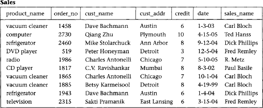
Figure 6.1 Single table database
Such a situation is shown in Figure 6.1, where products, salespersons, customers, and orders are all stored in a single table called Sales. In this table, we see that certain product and customer information is stored redundantly, wasting storage space. Certain queries, such as “Which customers ordered vacuum cleaners last month?” would require a search of the entire table. Also, updates such as changing the address of the customer Dave Bachmann would require changing many rows. Finally, deleting an order by a valued customer such as Qiang Zhu (who bought an expensive computer), if that is his only outstanding order, deletes the only copy of his address and credit rating as a side effect. Such information may be difficult (or sometimes impossible) to recover. These problems also occur for situations in which the database has already been set up as a collection of many tables, but some of the tables are still too large.
If we had a method of breaking up such a large table into smaller tables so that these types of problems would be eliminated, the database would be much more efficient and reliable. Classes of relational database schemes or table definitions, called normal forms, are commonly used to accomplish this goal. The creation of a normal form database table is called normalization. Normalization is accomplished by analyzing the interdependencies among individual attributes associated with those tables and taking projections (subsets of columns) of larger tables to form smaller ones.
Let us first review the basic normal forms, which have been well established in the relational database literature and in practice.
6.1.1 First Normal Form
Relational database tables, such as the Sales table illustrated in Figure 6.1, have only atomic values for each row and for each column. Such tables are considered to be in first normal form, the most basic level of normalized tables.
To better understand the definition for 1NF, it helps to know the difference between a domain, an attribute, and a column. A domain is the set of all possible values for a particular type of attribute, but may be used for more than one attribute. For example, the domain of people’s names is the underlying set of all possible names that could be used for either customer-name or salesperson-name in the database table in Figure 6.1. Each column in a relational table represents a single attribute, but in some cases more than one column may refer to different attributes from the same domain. When this occurs, the table is still in 1NF because the values in the table are still atomic. In fact, standard SQL assumes only atomic values and a relational table is by default in 1NF. A nice explanation of this is given in Muller [1999].
6.1.2 Superkeys, Candidate Keys, and Primary Keys
A table in 1NF often suffers from data duplication, update performance, and update integrity problems, as noted above. To understand these issues better, however, we must define the concept of a key in the context of normalized tables. A superkey is a set of one or more attributes, which, when taken collectively, allows us to identify uniquely an entity or table. Any subset of the attributes of a superkey that is also a superkey, and not reducible to another superkey, is called a candidate key. A primary key is selected arbitrarily from the set of candidate keys to be used in an index for that table.
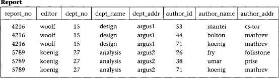
Figure 6.2 Report table
As an example, in Figure 6.2 a composite of all the attributes of the table forms a superkey because duplicate rows are not allowed in the relational model. Thus, a trivial superkey is formed from the composite of all attributes in a table. Assuming that each department address (dept_addr) in this table is single valued, we can conclude that the composite of all attributes except dept_addr is also a superkey. Looking at smaller and smaller composites of attributes and making realistic assumptions about which attributes are single valued, we find that the composite (report_no, author_id) uniquely determines all the other attributes in the table and is therefore a superkey. However, neither report_no nor author_id alone can determine a row uniquely, and the composite of these two attributes cannot be reduced and still be a superkey. Thus, the composite (report_no, author_id) becomes a candidate key. Since it is the only candidate key in this table, it also becomes the primary key.
A table can have more than one candidate key. If, for example, in Figure 6.2, we had an additional column for author_ssn, and the composite of report_no and author_ssn uniquely determine all the other attributes of the table, then both (report_no, author_id) and (report_no, author_ssn) would be candidate keys. The primary key would then be an arbitrary choice between these two candidate keys.
Other examples of multiple candidate keys can be seen in Figure 5.5 (see Chapter 5). In Figure 5.5a the table uses_notebook has three candidate keys: (emp_id, project_name), (emp_id, notebook_no), and (project_name, notebook_no); and in Figure 5.5b the table assigned_to has two candidate keys: (emp_id, loc_name) and (emp_id, project_name). Figures 5.5c and 5.5d each have only a single candidate key.
6.1.3 Second Normal Form
To explain the concept of second normal form (2NF) and higher, we introduce the concept of functional dependence, which was briefly described in Chapter 2. The property of one or more attributes that uniquely determine the value of one or more other attributes is called functional dependence. Given a table (R), a set of attributes (B) is functionally dependent on another set of attributes (A) if, at each instant of time, each A value is associated with only one B value. Such a functional dependence is denoted by A -> B. In the preceding example from Figure 6.2, let us assume we are given the following functional dependencies for the table report:
report: report_no -> editor, dept_no
dept_no -> dept_name, dept_addr
author_id -> author_name, author_addr
Definition. A table is in second normal form (2NF) if and only if it is in 1NF and every nonkey attribute is fully dependent on the primary key. An attribute is fully dependent on the primary key if it is on the right side of an FD for which the left side is either the primary key itself or something that can be derived from the primary key using the transitivity of FDs.
An example of a transitive FD in report is the following:
dept_no -> dept_name
Therefore we can derive the FD (report_no -> dept_name), since dept_name is transitively dependent on report_no.
Continuing our example, the composite key in Figure 6.2, (report_no, author_id), is the only candidate key and is therefore the primary key. However, there exists one FD (dept_no -> dept_name, dept_addr) that has no component of the primary key on the left side, and two FDs (report_no -> editor, dept_no and author_id -> author_name, author_addr) that contain one component of the primary key on the left side, but not both components. As such, report does not satisfy the condition for 2NF for any of the FDs.
Consider the disadvantages of 1NF in table report. Report_no, editor, and dept_no are duplicated for each author of the report. Therefore, if the editor of the report changes, for example, several rows must be updated. This is known as the update anomaly, and it represents a potential degradation of performance due to the redundant updating. If a new editor is to be added to the table, it can only be done if the new editor is editing a report: both the report number and editor number must be known to add a row to the table, because you cannot have a primary key with a null value in most relational databases. This is known as the insert anomaly. Finally, if a report is withdrawn, all rows associated with that report must be deleted. This has the side effect of deleting the information that associates an author_id with author_name and author_addr. Deletion side effects of this nature are known as delete anomalies. They represent a potential loss of integrity, because the only way the data can be restored is to find the data somewhere outside the database and insert it back into the database. All three of these anomalies represent problems to database designers, but the delete anomaly is by far the most serious because you might lose data that cannot be recovered.
These disadvantages can be overcome by transforming the 1NF table into two or more 2NF tables by using the projection operator on the subset of the attributes of the 1NF table. In this example we project report over report_no, editor, dept_no, dept_name, and dept_addr to form report1; and project report over author_id, author_name, and author_addr to form report2; and finally project report over report_no and author_id to form report3. The projection of report into three smaller tables has preserved the FDs and the association between report_no and author_no that was important in the original table. Data for the three tables is shown in Figure 6.3. The FDs for these 2NF tables are:
report1: report_no -> editor, dept_no
dept_no -> dept_name, dept_addr
report2: author_id -> author_name, author_addr
report3: report_no, author_id is a candidate key (no FDs)
We now have three tables that satisfy the conditions for 2NF, and we have eliminated the worst problems of 1NF, especially integrity (the delete anomaly). First, editor, dept_no, dept_name, and dept_addr are no longer duplicated for each author of a report. Second, an editor change results in only an update to one row for report1. And third, the most important, the deletion of the report does not have the side effect of deleting the author information.

Figure 6.3 2NF tables
Not all performance degradation is eliminated, however; report_no is still duplicated for each author, and deletion of a report requires updates to two tables (report 1 and report3) instead of one. However, these are minor problems compared to those in the 1NF table report.
Note that these three report tables in 2NF could have been generated directly from an ER (or UML) diagram that equivalently modeled this situation with entities Author and Report and a many-to-many relationship between them.
6.1.4 Third Normal Form
The 2NF tables we established in the previous section represent a significant improvement over 1NF tables. However, they still suffer from the same types of anomalies as the 1NF tables although for different reasons associated with transitive dependencies. If a transitive (functional) dependency exists in a table, it means that two separate facts are represented in that table, one fact for each functional dependency involving a different left side. For example, if we delete a report from the database, which involves deleting the appropriate rows from report1 and report3 (see Figure 6.3), we have the side effect of deleting the association between dept_no, dept_name, and dept_addr as well. If we could project table report1 over report_no, editor, and dept_no to form table report11, and project report1 over dept_no, dept_name, and dept_addr to form table report12, we could eliminate this problem. Example tables for report11 and report12 are shown in Figure 6.4.
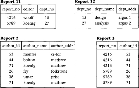
Figure 6.4 3NF tables
Definition. A table is in third normal form (3NF) if and only if for every nontrivial functional dependency X->A, where X and A are either simple or composite attributes, one of two conditions must hold. Either attribute X is a superkey, or attribute A is a member of a candidate key. If attribute A is a member of a candidate key, A is called a prime attribute. Note: a trivial FD is of the form YZ->Z.
In the preceding example, after projecting report1 into report11 and report12 to eliminate the transitive dependency report_no -> dept_no -> dept_name, dept_addr, we have the following 3NF tables and their functional dependencies (and example data in Figure 6.4):
report11: report_no -> editor, dept_no
report12: dept_no -> dept_name, dept_addr
report2: author_id -> author_name, author_addr
report3: report_no, author_id is a candidate key (no FDs)
6.1.5 Boyce-Codd Normal Form
3NF, which eliminates most of the anomalies known in databases today, is the most common standard for normalization in commercial databases and CASE tools. The few remaining anomalies can be eliminated by the Boyce-Codd normal form (BCNF) and higher normal forms defined here and in Section 6.5. BCNF is considered to be a strong variation of 3NF.
Definition. A table R is in Boyce-Codd normal form (BCNF) if for every nontrivial FD X->A, X is a superkey.
BCNF is a stronger form of normalization than 3NF because it eliminates the second condition for 3NF, which allowed the right side of the FD to be a prime attribute. Thus, every left side of an FD in a table must be a superkey. Every table that is BCNF is also 3NF, 2NF, and 1NF, by the previous definitions.
The following example shows a 3NF table that is not BCNF. Such tables have delete anomalies similar to those in the lower normal forms.
Assertion 1. For a given team, each employee is directed by only one leader. A team may be directed by more than one leader.
emp_name, team_name -> leader_name
Assertion 2. Each leader directs only one team.
leader_name -> team_name
This table is 3NF with a composite candidate key emp_id, team_id:

The team table has the following delete anomaly: if Sutton drops out of the Condors team, then we have no record of Bachmann leading the Condors team. As shown by Date [1999], this type of anomaly cannot have a lossless decomposition and preserve all FDs. A lossless decomposition requires that when you decompose the table into two smaller tables by projecting the original table over two overlapping subsets of the scheme, the natural join of those subset tables must result in the original table without any extra unwanted rows. The simplest way to avoid the delete anomaly for this kind of situation is to create a separate table for each of the two assertions. These two tables are partially redundant, enough so to avoid the delete anomaly. This decomposition is lossless (trivially) and preserves functional dependencies, but it also degrades update performance due to redundancy, and necessitates additional storage space. The trade-off is often worth it because the delete anomaly is avoided.
6.2 The Design of Normalized Tables: A Simple Example
The example in this section is based on the ER diagram in Figure 6.5 and the FDs given below. In general, FDs can be given explicitly, derived from the ER diagram, or derived from intuition (that is, from experience with the problem domain).
Our objective is to design a relational database schema that is normalized to at least 3NF and, if possible, minimize the number of tables required. Our approach is to apply the definition of third normal form (3NF) in Section 6.1.4 to the FDs given above, and create tables that satisfy the definition.
If we try to put FDs 1 through 6 into a single table with the composite candidate key (and primary key) (emp_id, start_date), we violate the 3NF definition, because FDs 2 through 6 involve left sides of FDs that are not superkeys. Consequently, we need to separate 1 from the rest of the FDs. If we then try to combine 2 through 6, we have many transitivities. Intuitively, we know that 2, 3, 4, and 5 must be separated into different tables because of transitive dependencies. We then must decide whether 5 and 6 can be combined without loss of 3NF; this can be done because mgr_id and dept_no are mutually dependent and both attributes are superkeys in a combined table. Thus, we can define the following tables by appropriate projections from 1 through 6.
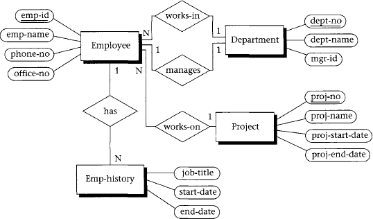
Figure 6.5 ER diagram for employee database
| emp_hist: | emp_id, start_date -> job_title, end_date |
| employee: | emp_id -> emp_name, phone_no, proj_no, dept_no |
| phone: | phone_no -> office_no |
| project: | proj_no -> proj_name, proj_start_date, proj_end_date |
| department: | dept_no -> dept_name, mgr_id mgr_id -> dept_no |
This solution, which is BCNF as well as 3NF, maintains all the original FDs. It is also a minimum set of normalized tables. In Section 6.4, we will look at a formal method of determining a minimum set that we can apply to much more complex situations.
Alternative designs may involve splitting tables into partitions for volatile (frequently updated) and passive (rarely updated) data, consolidating tables to get better query performance, or duplicating data in different tables to get better query performance without losing integrity. In summary, the measures we use to assess the trade-offs in our design are:
- Query performance (time)
- Update performance (time)
- Storage performance (space)
- Integrity (avoidance of delete anomalies)
6.3 Normalization of Candidate Tables Derived from ER Diagrams
Normalization of candidate tables [step II(d) in the database life cycle] is accomplished by analyzing the FDs associated with those tables: explicit FDs from the database requirements analysis (Section 6.2), FDs derived from the ER diagram, and FDs derived from intuition.
Primary FDs represent the dependencies among the data elements that are keys of entities, that is, the interentity dependencies. Secondary FDs, on the other hand, represent dependencies among data elements that comprise a single entity, that is, the intraentity dependencies. Typically, primary FDs are derived from the ER diagram, and secondary FDs are obtained explicitly from the requirements analysis. If the ER constructs do not include nonkey attributes used in secondary FDs, the data requirements specification or data dictionary must be consulted. Table 6.1 shows the types of primary FDs derivable from each type of ER construct.
Table 6.1 Primary FDs Derivable from ER Relationship Constructs

Each candidate table will typically have several primary and secondary FDs uniquely associated with it that determine the current degree of normalization of the table. Any of the well-known techniques for increasing the degree of normalization can be applied to each table to the desired degree stated in the requirements specification. Integrity is maintained by requiring the normalized table schema to include all data dependencies existing in the candidate table schema.
Any table B that is subsumed by another table A can potentially be eliminated. Table B is subsumed by another table A when all the attributes in B are also contained in A, and all data dependencies in B also occur in A. As a trivial case, any table containing only a composite key and no nonkey attributes is automatically subsumed by any other table containing the same key attributes, because the composite key is the weakest form of data dependency. If, however, tables A and B represent the supertype and subtype cases, respectively, of entities defined by the generalization abstraction, and A subsumes B because B has no additional specific attributes, the designer must collect and analyze additional information to decide whether or not to eliminate B.
A table can also be subsumed by the construction of a join of two other tables (a “join” table). When this occurs, the elimination of a subsumed table may result in the loss of retrieval efficiency, although storage and update costs will tend to be decreased. This trade-off must be further analyzed during physical design with regard to processing requirements to determine whether elimination of the subsumed table is reasonable.
To continue our example company personnel and project database, we want to obtain the primary FDs by applying the rules in Table 6.1 to each relationship in the ER diagram in Figure 4.3. The results are shown in Table 6.2.
Next we want to determine the secondary FDs. Let us assume that the dependencies in Table 6.3 are derived from the requirements specification and intuition.
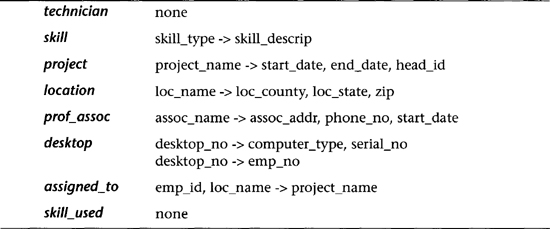
Normalization of the candidate tables is accomplished next. In Table 6.4 we bring together the primary and secondary FDs that apply to each candidate table. We note that for each table except employee, all attributes are functionally dependent on the primary key (denoted by the left side of the FDs) and are thus BCNF. In the case of table employee, we note that spouse_id determines emp_id and emp_id is the primary key; thus spouse_id can be shown to be a superkey (see Superkey Rule 2 in Section 6.4). Therefore, employee is found to be BCNF.
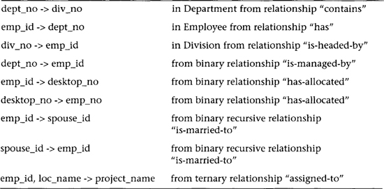
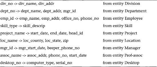
Table 6.3 Secondary FDs Derived from the Requirements Specification
In general, we observe that candidate tables, like the ones shown in Table 6.4, are fairly good indicators of the final schema and normally require very little refinement to get to 3NF or BCNF. This observation is important—good initial conceptual design usually results in tables that are already normalized or are very close to being normalized, and thus the normalization process is usually a simple task.
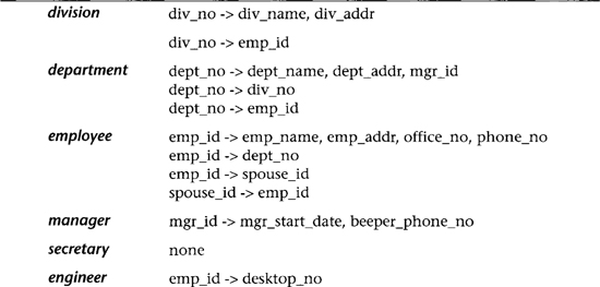
Table 6.4 Candidate Tables (and FDs) from ER Diagram Transformation
6.4 Determining the Minimum Set of 3NF Tables
A minimum set of 3NF tables can be obtained from a given set of FDs by using the well-known synthesis algorithm developed by Bernstein [1976]. This process is particularly useful when you are confronted with a list of hundreds or thousands of FDs that describe the semantics of a database. In practice, the ER modeling process automatically decomposes this problem into smaller subproblems: the attributes and FDs of interest are restricted to those attributes within an entity (and its equivalent table) and any foreign keys that might be imposed upon that table. Thus, the database designer will rarely have to deal with more than ten or twenty attributes at a time, and in fact most entities are initially defined in 3NF already. For those tables that are not yet in 3NF, only minor adjustments will be needed in most cases.
In the following text we briefly describe the synthesis algorithm for those situations where the ER model is not useful for the decomposition. In order to apply the algorithm, we make use of the well-known Armstrong axioms, which define the basic relationships among FDs.
Inference rules (Armstrong axioms)
These axioms can be used to derive two practical rules of thumb for deriving superkeys of tables where at least one superkey is already known.
Superkey Rule 1. Any FD involving all attributes of a table defines a superkey as the left side of the FD.
Given: Any FD containing all attributes in the table R(W, X, Y, Z), i.e., XY -> WZ.
Proof:
Superkey Rule 2. Any attribute that functionally determines a superkey of a table is also a superkey for that table.
Given: Attribute A is a superkey for table R(A, B, C, D, E), and E -> A.
Proof:
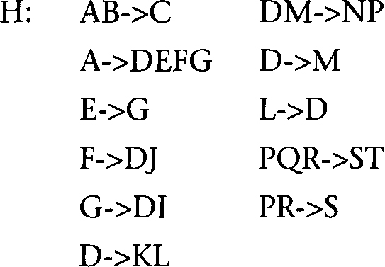
Before we can describe the synthesis algorithm, we must define some important concepts. Let H be a set of FDs that represents at least part of the known semantics of a database. The closure of H, specified by H+, is the set of all FDs derivable from H using the Armstrong axioms or inference rules. For example, we can apply the transitivity rule to the following FDs in set H:
A -> B, B -> C, A -> C, and C -> D
to derive the FDs A -> D and B -> D. All six FDs constitute the closure H+. A cover of H, called H’, is any set of FDs from which H+ can be derived. Possible covers for this example are:
A nonredundant cover of H is a cover of H that contains no proper subset of FDs, which is also a cover. The synthesis algorithm requires nonredundant covers.
3NF Synthesis Algorithm
Given a set of FDs, H, we determine a minimum set of tables in 3NF.
From this point the process of arriving at the minimum set of 3NF tables consists of five steps:
Now we discuss each step in turn, in terms of the preceding set of FDs, H.
Step 1. Elimination of Extraneous Attributes
The first task is to get rid of extraneous attributes in the left sides of the FDs.
The following two relationships (rules) among attributes on the left side of an FD provide the means to reduce the left side to fewer attributes.
Reduction Rule 1. XY->Z and X->Z => Y is extraneous on the left side (applying the reflexivity and transitivity axioms).
Reduction Rule 2. XY->Z and X->Y => Y is extraneous; therefore X->Z (applying the pseudotransitivity axiom).
Applying these reduction rules to the set of FDs in H, we get:
DM->NP and D->M => D->NP
PQR->ST and PR->S => PQR->T
Step 2. Search for a Nonredundant Cover
We must eliminate any FD derivable from others in H using the inference rules.
Transitive FDs to be eliminated:
A->E and E->G => eliminate A->G
A->F and F->D => eliminate A->D
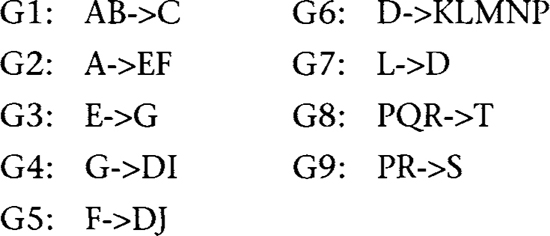
Step 3. Partitioning of the Nonredundant Cover
To partition the nonredundant cover into groups so that all FDs with the same left side are in one group, we must separate the nonfully functional dependencies and transitive dependencies into separate tables. At this point we have a feasible solution for 3NF tables, but it is not necessarily the minimum set.
These nonfully functional dependencies must be put into separate tables:
AB->C
A->EF
Groups with the same left side:
Step 4. Merge of Equivalent Keys (Merge of Tables)
In this step we merge groups with left sides that are equivalent (for example, X->Y and Y->X imply that X and Y are equivalent). This step produces a minimum set.
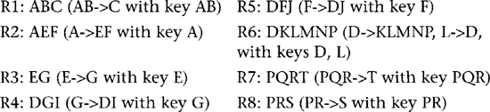
In this example, note that G7 (L->D) has a subset of the attributes of G6 (D->KLMNP). Therefore, we merge to a single table, R6, with FDs D->KLMNP and L->D, because it satisfies 3NF: D is a superkey by Superkey Rule 1, and L is a superkey by Superkey Rule 2.
Step 5. Definition of the Minimum Set of Normalized Tables
The minimum set of normalized tables has now been computed. We define them below in terms of the table name, the attributes in the table, the FDs in the table, and the candidate keys for that table:
Note that this result is not only 3NF, but also BCNF, which is very frequently the case. This fact suggests a practical algorithm for a (near) minimum set of BCNF tables: Use Bernstein’s algorithm to attain a minimum set of 3NF tables, then inspect each table for further decomposition (or partial replication, as shown in Section 6.1.5) to BCNF.
6.5 Fourth and Fifth Normal Forms
Normal forms up to BCNF were defined solely on FDs, and, for most database practitioners, either 3NF or BCNF is a sufficient level of normalization. However, there are in fact two more normal forms that are needed to eliminate the rest of the currently known anomalies. In this section, we will look at different types of constraints on tables: multivalued dependencies and join dependencies. If these constraints do not exist in a table, which is the most common situation, then any table in BCNF is automatically in fourth normal form (4NF), and fifth normal form (5NF) as well. However, when these constraints do exist, there may be further update (especially delete) anomalies that need to be corrected. First, we must define the concept of multivalued dependency.
6.5.1 Multivalued Dependencies
An MVD X ->> Y is trivial if Y is a subset of X, or if X union Y = RS. Finally, an FD implies an MVD, which implies that a single row with a given value of X is also an MVD, albeit a trivial form.
The following examples show where an MVD does and does not exist in a table. In R1, the first four rows satisfy all conditions for the MVDs X->>Y and X->>Z. Note that MVDs appear in pairs because of the cross-product type of relationship between Y and Z=RS-Y as the two right sides of the two MVDs. The fifth and sixth rows of R1 (when the X value is 2) satisfy the row interchange conditions in the above definition. In both rows, the Y value is 2, so the interchanging of Y values is trivial. The seventh row (3,3,3) satisfies the definition trivially.
In table R2, however, the Y values in the fifth and sixth rows are different (1 and 2), and interchanging the 1 and 2 values for Y results in a row (2,2,2) that does not appear in the table. Thus, in R2 there is no MVD between X and Y or between X and Z, even though the first four rows satisfy the MVD definition. Note that for the MVD to exist, all rows must satisfy the criterion for an MVD.
Table R3 contains the first three rows that do not satisfy the criterion for an MVD, since changing Y from 1 to 2 in the second row results in a row that does not appear in the table. Similarly, changing Z from 1 to 2 in the third row results in a nonappearing row. Thus, R3 does not have any MVDs between X and Y or between X and Z.
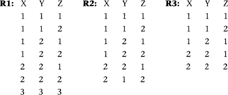
By the same argument, in table R1 we have the MVDs Y->> X and Y->>Z, but none with Z on the left side. Tables R2 and R3 have no MVDs at all.
The following inference rules for MVDs are somewhat analogous to the inference rules for functional dependencies given in Section 6.4 [Beeri, Fagin, and Howard, 1977]. They are quite useful in the analysis and decomposition of tables into 4NF.
Multivalued Dependency Inference Rules

6.5.2 Fourth Normal Form
The goal of 4NF is to eliminate nontrivial MVDs from a table by projecting them onto separate smaller tables, and thus to eliminate the update anomalies associated with the MVDs. This type of normal form is reasonably easy to attain if you know where the MVDs are. In general, MVDs must be defined from the semantics of the database; they cannot be determined from just looking at the data. The current set of data can only verify whether your assumption about an MVD is currently true or not, but this may change each time the data is updated.

Figure 6.6 Ternary relationship with multiple interpretations
Definition. A table R is in fourth normal form (4NF) if and only if it is in BCNF and, whenever there exists an MVD in R (say X ->> Y), at least one of the following holds: the MVD is trivial, or X is a superkey for R.
Applying this definition to the three tables in the example in the previous section, we see that R1 is not in 4NF because at least one nontrivial MVD exists and no single column is a superkey. In tables R2 and R3, however, there are no MVDs. Thus these two tables are at least 4NF.
As an example of the transformation of a table that is not in 4NF to two tables that are in 4NF, we observe the ternary relationship skill-required, shown in Figure 6.6. The relationship skill-required is defined as follows: “An employee must have all the required skills needed for a project to work on that project.” For example, in Table 6.5 the project with proj_no = 3 requires skill types A and B by all employees (see employees 101 and 102). The table skill_required has no FDs, but it does have several nontrivial MVDs, and is therefore only in BCNF. In such a case it can have a lossless decomposition into two many-to-many binary relationships between the entities Employee and Project, and Project and Skill. Each of these two new relationships represents a table in 4NF. It can also have a lossless decomposition resulting in a binary many-to-many relationship between the entities Employee and Skill, and Project and Skill.
A two-way lossless decomposition occurs when skill_required is projected over (emp_id, proj_no) to form skill_reql and projected over (proj_no, skill_type) to form skill_req3. Projection over (emp_id, proj_no) to form skill_req1 and over (emp_id, skill_type) to form skill_req2, however, is not lossless. A three-way lossless decomposition occurs when skill_required is projected over (emp_id, proj_no), (emp_id, skill_type), and (proj_no, skill_type).

Table 6.5 The Table skill_required and Its Three Projections
Tables in 4NF avoid certain update anomalies (or inefficiences). For instance, a delete anomaly exists when two independent facts get tied together unnaturally so that there may be bad side effects of certain deletes. For example, in skill_required, the last row of a skill_type may be lost if an employee is temporarily not working on any projects. An update inefficiency may occur when adding a new project in skill_required, which requires insertions for many rows to include all the required skills for that new project. Likewise, loss of a project requires many deletions. These inefficiencies are avoided when skill_required is decomposed into skill_reql and skill_req3. In general (but not always), decomposition of a table into 4NF tables results in less data redundancy.
6.5.3 Decomposing Tables to 4NF
Algorithms to decompose tables into 4NF are difficult to develop. Let’s look at some straightforward approaches to 4NF from BCNF and lower normal forms. First, if a table is BCNF, it either has no FDs, or each FD is characterized by its left side being a superkey. Thus, if the only MVDs in this table are derived from its FDs, they have only superkeys as their left sides, and the table is 4NF by definition. If, however, there are other nontrivial MVDs whose left sides are not superkeys, the table is only in BCNF and must be decomposed to achieve higher normalization.
The basic decomposition process from a BCNF table is defined by selecting the most important MVD (or if that is not possible, then by selecting one arbitrarily), defining its complement MVD, and decompose the table into two tables containing the attributes on the left and right sides of that MVD and its complement. This type of decomposition is lossless because each new table is based on the same attribute, which is the left side of both MVDs. The same MVDs in these new tables are now trivial because they contain every attribute in the table. However, other MVDs may be still present, and more decompositions by MVDs and their complements may be necessary. This process of arbitrary selection of MVDs for decomposition is continued until only trivial MVDs exist, leaving the final tables in 4NF.
As an example, let R(A, B, C, D, E, F) with no FDs, and with MVDs A ->> B and CD ->> EF. The first decomposition of R is into two tables R1(A, B) and R2(A, C, D, E, F) by applying the MVD A ->> B and its complement A ->> CDEF. Table R1 is now 4NF, because A ->> B is trivial and is the only MVD in the table. Table R2, however, is still only BCNF, because of the nontrivial MVD CD ->> EF. We then decompose R2 into R21(C, D, E, F) and R22(C, D, A) by applying the MVD CD ->> EF and its complement CD ->> A. Both R21 and R22 are now 4NF. If we had applied the MVD complement rule in the opposite order, using CD ->> EF and its complement CD ->> AB first, the same three 4NF tables would result from this method. However, this does not occur in all cases; it only occurs in those tables where the MVDs have no intersecting attributes.
This method, in general, has the unfortunate side effect of potentially losing some or all of the FDs and MVDs. Therefore, any decision to transform tables from BCNF to 4NF must take into account the trade-off between normalization and the elimination of delete anomalies, and the preservation of FDs and possibly MVDs. It should also be noted that this approach derives a feasible, but not necessarily a minimum, set of 4NF tables.
A second approach to decomposing BCNF tables is to ignore the MVDs completely and split each BCNF table into a set of smaller tables, with the candidate key of each BCNF table being the candidate key of a new table and the nonkey attributes distributed among the new tables in some semantically meaningful way. This form of decomposing by candidate key (that is, superkey) is lossless because the candidate keys uniquely join; it usually results in the simplest form of 5NF tables, those with a candidate key and one nonkey attribute, and no MVDs. However, if one or more MVDs still exist, further decomposition must be done with the MVD/MVD-complement approach given above. The decomposition by candidate keys preserves FDs, but the MVD/MVD-complement approach does not preserve either FDs or MVDs.
Tables that are not yet in BCNF can also be directly decomposed into 4NF using the MVD/MVD-complement approach. Such tables can often be decomposed into smaller minimum sets than those derived from transforming into BCNF first and then 4NF, but with a greater cost of lost FDs. In most database design situations, it is preferable to develop BCNF tables first, then evaluate the need to normalize further while preserving the FDs.
6.5.4 Fifth Normal Form
Definition. A table R is in fifth normal form (5NF) or project-join normal form (PJ/NF) if and only if every join dependency in R is implied by the keys of R.
As we recall, a lossless decomposition of a table implies that it can be decomposed by two or more projections, followed by a natural join of those projections (in any order) that results in the original table, without any spurious or missing rows. The general lossless decomposition constraint, involving any number of projections, is also known as a join dependency (JD). A join dependency is illustrated by the following example: in a table R with n arbitrary subsets of the set of attributes of R, R satisfies a join dependency over these n subsets if and only if R is equal to the natural join of its projections on them. A JD is trivial if one of the subsets is R itself.
5NF or PJ/NF requires satisfaction of the membership algorithm [Fagin, 1979], which determines whether a JD is a member of the set of logical consequences of (can be derived from) the set of key dependencies known for this table. In effect, for any 5NF table, every dependency (FD, MVD, JD) is determined by the keys. As a practical matter we note that because JDs are very difficult to determine in large databases with many attributes, 5NF tables are not easily derivable, and logical database design typically produces BCNF tables.
We should also note that by the preceding definitions, just because a table is decomposable does not necessarily mean it is not 5NF. For example, consider a simple table with four attributes (A, B, C, D), one FD (A->BCD), and no MVDs or JDs not implied by this FD. It could be decomposed into three tables, A->B, A->C, and A->D, all based on the same superkey A; however, it is already in 5NF without the decomposition. Thus, the decomposition is not required for normalization. On the other hand, decomposition can be a useful tool in some instances for performance improvement.

Table 6.6 The Table skill_in_common and Its Three Projections
The following example demonstrates that a table representing a ternary relationship may not have any two-way lossless decompositions; however, it may have a three-way lossless decomposition, which is equivalent to three binary relationships, based on the three possible projections of this table. This situation occurs in the relationship skill-in-common (Figure 6.6), which is defined as “The employee must apply the intersection of his or her available skills with the skills needed to work on certain projects.” In this example, skill-in-common is less restrictive than skill-required because it allows an employee to work on a project even if he or she does not have all the skills required for that project.
As Table 6.6 shows, the three projections of skill_in_common result in a three-way lossless decomposition. There are no two-way lossless decompositions and no MVDs; thus, the table skill_in_common is in 4NF.
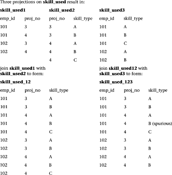
The ternary relationship in Figure 6.6 can be interpreted yet another way. The meaning of the relationship skill-used is “We can selectively record different skills that each employee applies to working on individual projects.” It is equivalent to a table in 5NF that cannot be decomposed into either two or three binary tables. Note by studying Table 6.7 that the associated table, skill_used, has no MVDs or JDs.
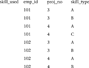
Table 6.7 The Table skill_used, Its Three Projections, and Natural Joins of Its Projections
A table may have constraints that are FDs, MVDs, and JDs. An MVD is a special case of a JD. To determine the level of normalization of the table, analyze the FDs first to determine normalization through BCNF; then analyze the MVDs to determine which BCNF tables are also 4NF; then, finally, analyze the JDs to determine which 4NF tables are also 5NF.
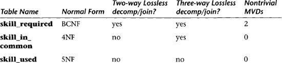
Table 6.8 Summary of Higher Normal Forms
A many-to-many-to-many ternary relationship is:
- BCNF if it can be replaced by two binary relationships
- 4NF if it can only be replaced by three binary relationships
- 5NF if it cannot be replaced in any way (and thus is a true ternary relationship)
We observe the equivalence between certain ternary relationships and the higher normal form tables transformed from those relationships. Ternary relationships that have at least one “one” entity cannot be decomposed (or broken down) into binary relationships, because that would destroy the one or more FDs required in the definition, as shown previously. A ternary relationship with all “many” entities, however, has no FDs, but in some cases may have MVDs, and thus have a lossless decomposition into equivalent binary relationships.
In summary, the three common cases that illustrate the correspondence between a lossless decomposition in a many-to-many-to-many ternary relationship table and higher normal forms in the relational model are shown in Table 6.8.
6.6 Summary
In this chapter, we defined the constraints imposed on tables—most commonly the functional dependencies or FDs. Based on these constraints, practical normal forms for database tables are defined: 1NF, 2NF, 3NF, and BCNF. All are based on the types of FDs present. In this chapter, a practical algorithm for finding the minimum set of 3NF tables is given.
The following statements summarize the functional equivalence between the ER model and normalized tables:
In summary, we observed that a good, methodical conceptual design procedure often results in database tables that are either normalized (BCNF) already, or can be normalized with very minor changes.
6.7 Literature Summary
Good summaries of normal forms can be found in Date [1999], Kent [1983], Dutka and Hanson [1989], and Smith [1985]. Algorithms for normal form decomposition and synthesis techniques are given in Bernstein [1976], Fagin [1977], and Maier [1983]. The earliest work in normal forms was done by Codd [1970, 1974].