
Mode analysis
Abstract
When a steel bar is hit by a hammer, a clear sound can be heard because the steel bar vibrates at its resonant frequency. If the bar is oscillated at this resonant frequency, it will be found that the vibration amplitude of the bar becomes very large. Therefore, when a machine is designed, it is important to know the resonant frequency of the machine. The analysis to obtain the resonant frequency and the vibration mode of an elastic body is called ‘mode analysis’.
The finite element method (FEM) analysis makes it possible to obtain the vibration mode for a various complex shape of an elastic body. In this chapter, vibration modes and resonant frequencies of a straight beam, a HDD suspension, a one axis moving table and a high-speed spindle using elastic hinges are solved by the ANSYS software.
Keywords
Mode analysis; Vibration mode; Resonant frequency; Type of elements
4.1 Introduction
When a steel bar is hit by a hammer, a clear sound can be heard because the steel bar vibrates at its resonant frequency. If the bar is oscillated at this resonant frequency, it will be found that the vibration amplitude of the bar becomes very large. Therefore, when a machine is designed, it is important to know the resonant frequency of the machine. The analysis to obtain the resonant frequency and the vibration mode of an elastic body is called ‘mode analysis’.
It is said that there are two methods for mode analysis. One is the theoretical analysis and the other is the finite element method (FEM). Theoretical analysis is usually used for a simple shape of an elastic body, such as a flat plate and a straight bar but theoretical analysis cannot give us the vibration mode for the complex shape of an elastic body. FEM analysis can obtain the vibration mode for it.
In this chapter, three examples are presented, which use beam elements, shell elements and solid elements, respectively, as shown in Fig. 4.1.

4.2 Mode analysis of a straight bar
4.2.1 Problem description
Obtain the lowest three vibration modes and resonant frequencies in the y direction of the straight steel bar shown in Fig. 4.2 when the bar can move only in the y direction.

Thickness of the bar is 0.005 m; width of the bar is 0.01 m; length of the bar is 0.09 m. Material of the bar is steel with Young's modulus, E = 206 GPa, and Poisson's ratio ν = 0.3. Density ρ = 7.8 × 10³ kg/m3.
Boundary condition: All freedoms are constrained at the left end.
4.2.2 Analytical solution
Before mode analysis is attempted using ANSYS, an analytical solution for resonant frequencies will be obtained to confirm the validity of ANSYS solution. The analytical solution of resonant frequencies for a cantilever beam in y direction is given by,

where length of the cantilever beam, L = 0.09 m, cross section area of the cantilever beam, A = 5 × 10− 5 m2,
Young's modulus E =206 GPa.
The area moment of inertia of the cross section of the beam is
Mass per unit width M = ρAL/L = ρA = 7.8 × 10³ kg/m3 × 5 × 10− 5 m2 = 0.39 kg/m.
λ1 = 1.875, λ2 = 4.694, λ3 = 7.855.
For that set of data the following solutions is obtained: f1 = 512.5 Hz; f2 = 3212 Hz; f3 = 8994 Hz.
Fig. 4.3 shows the vibration modes and the positions of nodes obtained by Eq. (4.1).

4.2.3 Model for FE analysis
4.2.3.1 Element type selection
In FEM analysis, it is very important to select a proper element type which influences the accuracy of solution, working time for model construction and CPU time. In this example, the two-dimensional elastic beam, as shown in Fig. 4.4, is selected for the following reasons:
- (a) Vibration mode is constrained in the two-dimensional plane.
- (b) Number of elements can be reduced; the time for model construction and CPU time are both shortened.

A two-dimensional elastic beam has three degrees of freedom at each node (i, j), which are translatory deformations in the x and y directions and rotational deformation around the z axis. This beam can be subject to extension or compression bending due to its length and the magnitude of the area moment of inertia of its cross section.
From the ANSYS Main Menu, select Preprocessor → Element Type → Add/Edit/Delete.
Then the Element Types window, as shown in Fig. 4.5, is opened.
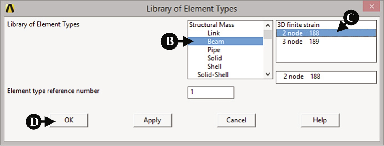
- 1. Click [A] Add. Then the Library of Element Types window as shown in Fig. 4.6 opens.
- 2. Select [B] Beam in the Library of Element Types table, and then select [C] 2 node 188.
- 3. Ensure Element type reference number is set to 1 and click the [D] OK button. Then the Library of Element Types window is closed.
- 4. Click the [E] Close button in the window of Fig. 4.7.


4.2.3.2 Sections for beam element
From the ANSYS Main Menu, select Preprocessor → Sections → Beam → Common Sections.
- 1. The Beam Tool window opens. Input beam1 to the [A] Name box, and select rectangular shape [B] in the Sub-Type box. Input the following values of [C] B = 0.005 and [D] H = 0.01, respectively, as shown in Fig. 4.8.
- 2. After inputting these values, click [E] OK.

4.2.3.3 Material properties
This section describes the procedure of defining the material properties of the beam element.
From the ANSYS Main Menu, select Preprocessor → Material Props → Material Models.
- 1. Click the above buttons in specified order and the Define Material Model Behavior window as shown in Fig. 4.9 opens.
- 2. Click the following terms in the window: [A] Structural → Linear → Elastic → Isotropic. As a result, the window of Linear Isotropic Properties for Material Number 1 as shown in Fig. 4.10 opens.
- 3. Input Young's modulus of 206e9 to the [B] EX box and Poisson ratio of 0.3 to the [C] PRXY box. Then click the [D] OK button.


Next, define the value of density of material.
- 1. Click the term [E] Density in Fig. 4.9 and the window Density for Material Number 1, Fig. 4.11, opens.
- 2. Input the value of density, 7800, to the [F] DENS box and click the [G] OK button. Finally, close the window Define Material Model Behavior by clicking the [H] X mark at the upper right corner).

4.2.3.4 Create keypoints
To draw a cantilever beam for analysis, the method of using keypoints is described.
From the ANSYS Main Menu, select Preprocessor → Modeling → Create → Keypoints → In Active CS.
The Create Keypoints in Active Coordinate System window, Fig. 4.12, opens.
- 1. Input 1 to the [A] NPT Key Point number box, 0, 0, 0 to the [B] X,Y,Z Location in active CS box, and then click the [C] Apply button. Do not click the OK button at this stage. If you do, the window will be closed. In this case, open the Create Keypoints in Active Coordinate System window as shown in Fig. 4.13 and then proceed to step 2.
- 2. In the same window, input 2 to the [D] NPT Key Point number box, 0.09, 0, 0 to the [E] X,Y,Z Location in active CS box, and then click the [F] OK button.
- 3. After finishing the above steps, two keypoints appear in the window as shown in Fig. 4.14.


4.2.3.5 Create a line for beam element
By implementing the following steps, a line between two keypoints is created.
From the ANSYS Main Menu, select Preprocessor → Modeling → Create → Lines → Lines → Straight Line.
The window Create Straight Line, shown in Fig. 4.15, is opened.
- 1. Pick the keypoints, [A] 1 and [B] 2, shown in Fig. 4.16, and click the [C] OK button in the window Create Straight Line shown in Fig. 4.15. A line is created as shown in Fig. 4.16.


4.2.3.6 Create mesh in a line
From the ANSYS Main Menu, select Preprocessor → Meshing → Size Cntrls → Manual Size → Lines → All Lines.
The window Element Sizes on All Selected Lines, shown in Fig. 4.17, is opened.
- 1. Input [A] the number of 20 to the NDIV box. This means that a line is divided into 20 elements.
- 2. Click the [B] OK button and close the window.

From the ANSYS Graphic Window, the preview of the divided line is available, as shown in Fig. 4.18, but the line is not really divided at this stage.

From the ANSYS Main Menu, select Preprocessor → Meshing → Mesh → Lines.
The Mesh Lines window, shown in Fig. 4.19, opens.
- 1. Click [C] the line shown in the ANSYS Graphic Window, as seen in Fig. 4.18, and then the [D] OK button to finish dividing the line.

4.2.3.7 Boundary conditions
The left end of nodes is fixed in order to constrain the left end of the cantilever beam.
From the ANSYS Main Menu, select Solution → Define Loads → Apply → Structural → Displacement → On Nodes.
The Apply U, ROT on Nodes window, shown in Fig. 4.20, opens.
- 1. Pick [A] the node at the left end in Fig. 4.21 and click the [B] OK button. Then the window Apply U, ROT on Nodes, shown in Fig. 4.22, opens.
- 2. In order to set the boundary condition, select [C] All DOF in the Lab2 box. In the VALUE box, input 0, and then click the [E] OK button. After these steps, the ANSYS Graphic Window is changed as shown in Fig. 4.23.


In order to obtain the vibration modes only in the y direction, the following boundary conditions are set.
From the ANSYS Main Menu, select Solution → Define Loads → Apply → Structural → Displacement → On Lines.
The window Apply U, ROT on Nodes, shown in Fig. 4.24, opens.
- 3. Pick [A] the line in Fig. 4.25 and click the [B] OK button. Then the window Apply U, ROT on Lines, shown in Fig. 4.26, opens. Select [C] UZ in the Lab2 box. In the VALUE box, input 0, and then click the [E] Apply button. After these steps, the ANSYS Graphic Window is changed as shown in Fig. 4.27.
- 4. Pick [A] the line again as indicated in Fig. 4.25, and click the [B] OK button as shown in Fig. 4.28. Then the window Apply U, ROT on Lines, shown in Fig. 4.29, opens again. Select [C] ROTX in the Lab2 box. In the VALUE box input 0, and then click the [E] OK button. After these steps, the ANSYS Graphic Window is changed as shown in Fig. 4.30.


4.2.4 Execution of the analysis
4.2.4.1 Definition of the type of analysis
The following steps are used to define the type of analysis.
From the ANSYS Main Menu, select Solution → Analysis Type → New Analysis.
The New Analysis window, shown in Fig. 4.31, opens.
- 1. Check [A] Modal, and then click the [B] OK button.

In order to define the number of modes to extract, the following procedure is used.
From the ANSYS Main Menu, select Solution → Analysis Type → Analysis Options.
The Modal Analysis window, shown in Fig. 4.32, opens.
- 1. Check [C] Supernode of MODOPT and input [D] 3 in the No. of modes to extract box, then click the [E] OK button.
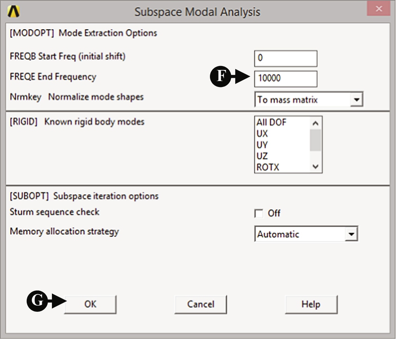
- 2. Then, the window Subspace Modal Analysis, shown in Fig. 4.33 opens. Input [F] 10000 in the FREQE box and click the [G] OK button.

4.2.4.2 Execute calculation
From the ANSYS Main Menu, select Solution → Solve → Current LS.
The Solve Current Load Step window, shown in Fig. 4.34, opens.
- 1. Click the [A] OK button to initiate calculation. When the Note window, shown in Fig. 4.35, appears, then the calculation is finished.
- 2. Click the [B] Close button and to close the window. The /STATUS Command window, shown in Fig. 4.36, also opens but this window can be closed by clicking [C] the mark X at the upper right-hand corner of the window.


4.2.5 Postprocessing
4.2.5.1 Read the calculated results of the first mode of vibration
From the ANSYS Main Menu, select General Postproc → Read Results → First Set.
4.2.5.2 Plot the calculated results
From the ANSYS Main Menu, select General Postproc → Plot Results → Deformed Shape.
The window Plot Deformed Shape, shown in Fig. 4.37, opens.
- 1. Select [A] Def + Undeformed and click [B] OK.
- 2. Calculated result for the first mode of vibration is displayed (ANSYS Graphic Window) as shown in Fig. 4.38. The resonant frequency is shown as FRQE at the upper left-hand side on the window.


4.2.5.3 Read the calculated results from the second and third modes of vibration
From the ANSYS Main Menu, select General Postproc → Read Results → Next Set.
Follow the same steps outlined in Section 4.2.5.2 and calculate the results for the second and third modes of vibration. The results are plotted in Figs 4.39 and 4.40.


4.3 Modal analysis of a suspension for hard disc drive
4.3.1 Problem description
A suspension of HDD has many resonant frequencies with various vibration modes and it is said that the vibration mode with large radial displacement causes the tracking error. So the suspension has to be operated with frequencies of less than this resonant frequency.
Obtain the resonant frequencies and determine the vibration mode with large radial displacement of the HDD suspension as shown in Fig. 4.41.

Material: Steel.
Young's modulus, E = 206 GPa, Poisson's ratio ν = 0.3.
Density ρ = 7.8 × 10³ kg/m3.
Boundary condition: All freedoms are constrained at the edge of a hole formed in the suspension.
4.3.2 Create a model for analysis
4.3.2.1 Element type selection
In this example, the three-dimensional elastic shell is selected for calculations as shown in Fig. 4.41. Shell element is very suitable for analysing the characteristics of thin material.
From the ANSYS Main Menu, select Preprocessor → Element Type → Add/Edit/Delete.
Then the Element Types window, as shown in Fig. 4.42, is opened.
- 1. Click [A] add. Then the Library of Element Types window as shown in Fig. 4.43 opens.
- 2. Select [B] Shell in the Library of Element Types table, and then select [C] 3D 8node 281.
- 3. Ensure the Element type reference number is set to 1 and click the [D] OK button. Then the window Library of Element Types is closed.
- 4. Click the [E] Close button in the window of Fig. 4.44.


4.3.2.2 Material properties
This section describes the procedure of defining the material properties of shell element.
From the ANSYS Main Menu, select Preprocessor → Material Props → Material Models.
- 1. Click the above buttons in order and the Define Material Model Behavior window opens, as shown in Fig. 4.9.
- 2. Double-click the following terms in the window: Structural → Linear → Elastic → Isotropic. Then the window Linear Isotropic Properties for Material Number 1, Fig. 4.45, opens.
- 3. Input Young's Modulus of 206e9 to the [A] EX box and Poisson ratio of 0.3 to the [B] PRXY box. Then click the [C] OK button.

Next, define the value of density of material.
- 1. Double-click the term Density, and the window Density for Material Number 1, Fig. 4.46, opens.
- 2. Input the value of Density, 7800, to the [D] DENS box and click the [E] OK button. Finally close the window Define Material Model Behavior by clicking the X mark at the upper right end.

4.3.2.3 Sections for shell element
From the ANSYS Main Menu, select Preprocessor → Sections → Shell → Lay-up → Add/Edit.
- 1. The window Create and Modify Shell Sections, shown in Fig. 4.47, opens. Input the thickness of Shell section, 5.e-5, to [A] Thickness and click the [B] OK button to close the window.

4.3.2.4 Create keypoints
To draw a suspension for analysis, the method using keypoints on the window are described in this section.
From the ANSYS Main Menu, select Preprocessor → Modeling → Create → Keypoints → In Active CS.
- 1. The window Create Keypoints in Active Coordinate System, shown in Fig. 4.48, opens.
- 2. Input [A] 0, -0.6e-3, 0 to the X, Y, Z Location in active CS box, and then click the [B] Apply button. Do not click the OK button at this stage. If any figure is not inputted into the [C] NPT Key Point number box, the number of key point is automatically assigned in order.
- 3. In the same window, input the values as shown in Table 4.1 in order. When all values are inputted, click the OK button.
- 4. Then all inputted keypoints appears on the ANSYS Graphic Window as shown in Fig. 4.49.


Table 4.1
| KP No. | X | Y | Z | KP No. | X | Y | Z |
|---|---|---|---|---|---|---|---|
| 1 | 0 | − 0.6e − 3 | 9 | 8.3e − 3 | − 0.8e − 3 | ||
| 2 | 8.3e − 3 | − 2.15e − 3 | 10 | 10.5e − 3 | − 0.8e − 3 | ||
| 3 | 8.3e − 3 | − 1.4e − 3 | 11 | 10.5e − 3 | 0.8e − 3 | ||
| 4 | 13.5e − 3 | − 1.4e − 3 | 12 | 8.3e − 3 | 0.8e − 3 | ||
| 5 | 13.5e − 3 | 1.4e − 3 | 13 | 0 | − 0.6e − 3 | 0.3e − 3 | |
| 6 | 8.3e − 3 | 1.4e − 3 | 14 | 8.3e − 3 | − 2.15e − 3 | 0.3e − 3 | |
| 7 | 8.3e − 3 | 2.15e − 3 | 15 | 8.3e − 3 | 2.15e − 3 | 0.3e − 3 | |
| 8 | 0 | 0.6e − 3 | 16 | 0 | 0.6e − 3 | 0.3e − 3 |

4.3.2.5 Create areas for suspension
Areas are created from keypoints by performing the following steps.
From the ANSYS Main Menu, select Preprocessor → Modeling → Create → Area → Arbitrary → Through KPs.
- 1. The Create Area thru KPs window, shown in Fig. 4.50, opens.
- 2. Pick the keypoints [A] 9, 10, 11, and 12 in Fig. 4.51 in order and click the [B] Apply button in Fig. 4.50. An area is created on the window as shown in Fig. 4.51.
- 3. By performing the same steps, other areas are made on the window. Click the keypoints listed in Table 4.2 and make other areas. When you make areas No. 3 and 4, you have to rotate the drawing of suspension, using PlotCtrls—Pan Zoom Rotate in the Utility Menu.
- 4. When all areas are made on the window, click the [C] OK button in Fig. 4.50. Then the drawing of the suspension in Fig. 4.52 appears.
- 5. From the ANSYS Main Menu, select Preprocessor → Modeling → Create → Area → Circle → Solid Circle.


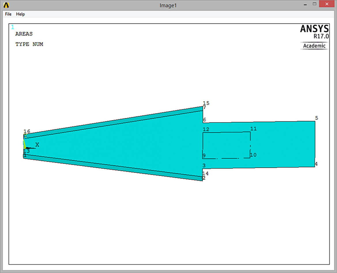
Table 4.2
| Area No. | Keypoint Number |
|---|---|
| 1 | 9, 10, 11, 12 |
| 2 | 1, 2, 3, 4, 5, 6, 7, 8 |
| 3 | 1, 2, 14, 13 |
| 4 | 8, 7, 15, 16 |
The Solid Circle Area window, shown in Fig. 4.53, opens. Input [D] the values of 12.0e-3, 0, and 0.6e-3 to the X, Y, and Radius boxes as shown in Fig. 4.53, respectively, and click the [E] OK button. Then the solid circle is made in the drawing of suspension as shown in Fig. 4.54.


4.3.2.6 Boolean operation
In order to make a spring region and the fixed region of the suspension, the rectangular and circle areas in the suspension are subtracted by Boolean operation.
From the ANSYS Main Menu, select Preprocessor → Modeling → Operate → Booleans → Subtract → Areas.
- 1. The Subtract Areas window, shown in Fig. 4.55, opens.
- 2. Click [A] the area of the suspension in the ANSYS Graphic Window as shown in Fig. 4.56 and click the [B] OK button, as in Fig. 4.55. Then click the [C] rectangular and [D] circular areas as shown in Fig. 4.57 and click the [B] OK button, as in Fig. 4.55. The drawing of the suspension appears as shown in Fig. 4.58.
- 3. In analysis, all areas have to be glued.


From the ANSYS Main Menu, select Preprocessor → Modeling → Operate → Booleans → Glue → Areas.
The Glue Areas window, shown in Fig. 4.59, opens. Click the [E] Pick All button.

4.3.2.7 Create mesh in areas
From the ANSYS Main Menu, select Preprocessor → Meshing → Size Cntrls → Manual Size → Areas → All Areas.
The window Element Sizes on All Selected Areas, shown in Fig. 4.60, opens.
- 1. Input [A] 0.0002 to the SIZE box. This means that areas are divided by meshes of edge length of 0.0002 m.
- 2. Click the [B] OK button and close the window.

From the ANSYS Main Menu, select Preprocessor → Meshing → Mesh → Areas → Free.
The Mesh Lines window, shown in Fig. 4.61, opens.
- 1. Click [C] Pick ALL and then the [D] OK button to finish dividing the areas as shown in Fig. 4.62.


4.3.2.8 Boundary conditions
The suspension is fixed at the edge of the circle.
From the ANSYS Main Menu, select Solution → Define Loads → Apply → Structural → Displacement → On Lines.
The window Apply U, ROT on Nodes, shown in Fig. 4.63, opens.
- 1. Pick [A] four lines included in the circle in Fig. 4.64 and click the [B] OK button in Fig. 4.63. Then the window Apply U, ROT on Lines, shown in Fig. 4.65, opens.
- 2. In order to set the boundary condition, select [C] All DOF in the Lab2 box. Input [D] 0 to the VALUE box, and then click the [E] OK button. After these steps, the ANSYS Graphic Window is changed as seen in Fig. 4.66.


4.3.3 Execute the analysis
4.3.3.1 Define the type of analysis
The following steps are performed to define the type of analysis.
From the ANSYS Main Menu, select Solution → Analysis Type → New Analysis.
The New Analysis window, shown in Fig. 4.67, opens.
- 1. Check [A] Modal, and then click the [B] OK button.

In order to define the number of modes to extract, the following steps are performed.
From the ANSYS Main Menu, select Solution → Analysis Type → Analysis Options.
The Modal Analysis window, shown in Fig. 4.68, opens.
- 1. Check [C] Subspace of MODOPT and input [D] 10 in the No. of modes to extract box, then click the [E] OK button.
- 2. The window Subspace Modal Analysis, as shown in Fig. 4.69, then opens. Input [F] 20000 in the FREQE box and click the [G] OK button.


4.3.3.2 Execute calculation
From the ANSYS Main Menu, select Solution → Solve → Current LS.
4.3.4 Postprocessing
4.3.4.1 Read the calculated results of the first mode of vibration
From the ANSYS Main Menu, select General Postproc → Read Results → First Set.
4.3.4.2 Plot the calculated results
From the ANSYS Main Menu, select General Postproc → Plot Results → Deformed Shape.
The Plot Deformed Shape window, shown in Fig. 4.70, opens.
- 1. Select [A] Def + Undeformed and click [B] OK.
- 2. The calculated result for the first mode of vibration appears on the ANSYS Graphic Window as shown in Fig. 4.71. The resonant frequency is shown as FRQE at the upper left side on the window.


4.3.4.3 Read the calculated results of higher modes of vibration
From the ANSYS Main Menu, select General Postproc → Read Results → Next Set.
Perform the same steps indicated in Section 4.2.4.2 and calculated results from the second mode to the sixth mode of vibration are displayed on the windows as shown in Figs 4.72–4.76.


4.4 Modal analysis of a one axis precision moving table using elastic hinges
4.4.1 Problem description
A one-axis table using elastic hinges has been often used in various precision equipment, and the position of a table is usually controlled at nanometer order accuracy using a piezoelectric actuator or a voice coil motor. Therefore, it is necessary to confirm the resonant frequency in order to determine the controllable frequency region.
Obtain the resonant frequency of a one-axis moving table using elastic hinges when the bottom of the table is fixed and a piezoelectric actuator is selected as an actuator.
Material: Steel, thickness of the table: 5 mm.
Young's modulus, E = 206 GPa, Poisson's ratio ν = 0.3.
Density ρ = 7.8 × 10³ kg/m3.
Boundary condition: All freedoms are constrained at the bottom of the table and the region A indicated in Fig. 4.77, where a piezoelectric actuator is glued.

4.4.2 Create a model for analysis
4.4.2.1 Select element type
In this example, the solid element is selected to analyse the resonant frequency of the moving table.
From the ANSYS Main Menu, select Preprocessor → Element Type → Add/Edit/Delete.
Then the Element Types window, as shown in Fig. 4.78, opens.
- 1. Click the [A] Add button. Then Library of Element Types window as shown in Fig. 4.79 opens.
- 2. Select [B] Solid in the Library of Element Types table, and then select [C] Quad 4node 182. Ensure the Element type reference number is set to 1 and click [D] Apply. Next, select [E] Brick 8node 185 as shown in Fig. 4.80.
- 3. Ensure the Element type reference number is set to 2 and click the [F] OK button. Then the Library of Element Types window is closed.
- 4. Click the [G] Close button in the window of Fig. 4.81 where the names of selected elements are indicated.


4.4.2.2 Material properties
This section describes the procedure of defining the material properties of solid element.
From the ANSYS Main Menu, select Preprocessor → Material Props → Material Models.
- 1. Click the above buttons in order and the window Define Material Model Behavior opens as shown in Fig. 4.82.
- 2. Double-click the following terms in the window: Structural → Linear → Elastic → Isotropic. Then the window Linear Isotropic Properties for Material Number 1 opens.
- 3. Input Young's Modulus of 206e9 to the EX box and Poisson ratio of 0.3 to the PRXY box.

Next, define the value of density of material.
- 1. Double-click the term Density, and the Density for Material Number 1 window opens.
- 2. Input the value of Density, 7800, to the DENS box and click the OK button. Finally close the Define Material Model Behavior window by clicking the X mark at the upper right end.
4.4.2.3 Create keypoints
To draw the moving table for analysis, the method using keypoints on the window are described in this section.
From the ANSYS Main Menu, select Preprocessor → Modeling → Keypoints → In Active CS.
The window Create Keypoints in Active Coordinate System, shown in Fig. 4.83, opens.
- 1. Input [A] 0, 0 to the X, Y, Z Location in active CS box, and then click the [B] Apply button. Do not click the OK button at this stage.
- 2. In the same window, input the values as shown in Table 4.3 in order. When all values are inputted, click the OK button.
- 3. Then all input keypoints appear on the ANSYS Graphic Window, as shown in Fig. 4.84.


4.4.2.4 Create areas for the table
Areas are created from keypoints by carrying out the following steps.
From the ANSYS Main Menu, select Preprocessor → Modeling → Create → Areas → Arbitrary → Through KPs.
The window Create Area thru KPs, shown in Fig. 4.85, opens.
- 1. Pick the keypoints, 1, 2, 3, and 4, in order and click the [A] Apply button in Fig. 4.85. Then pick keypoints 5, 6, 7, and 8, and click the [B] OK button. Fig. 4.86 appears.


From the ANSYS Main Menu, select Preprocessor → Modeling → Operate → Booleans → Subtract → Areas.
- 2. Click the area of KP no. 1–4 and the OK button. Then click the area of KP no. 5–8 and the OK button. The drawing of the table appears as shown in Fig. 4.87.

From the ANSYS Main Menu, select Preprocessor → Modeling → Create → Areas → Arbitrary → Through KPs.
- 3. Pick the keypoints 9, 10, 11, and 12 in order and click the [A] Apply button in Fig. 4.85. Then pick keypoints 13, 14, 15, and 16 and click the [B] OK button. Fig. 4.88 appears.

From the ANSYS Main Menu, select Preprocessor → Modeling → Operate → Booleans → Add → Areas.
The window Create Area thru KPs, shown in Fig. 4.89, opens.
- 4. Pick three areas on the ANSYS graphic window and click the [A] OK button. Then three areas are added as shown in Fig. 4.90.


From the ANSYS Main Menu, select Preprocessor → Modeling → Create → Area → Circle → Solid Circle.
The Solid Circle Area window, shown in Fig. 4.91, opens.
- 5. Input the values of 0, 12.2e-3, and 2.2e-3 to the X, Y, and Radius boxes as shown in Fig. 4.91 and click the [A] Apply button. Then continue to input the coordinates of the solid circle as shown in Table 4.4. When all values are inputted, the drawing of the table appears as shown in Fig. 4.92 Click the [B] OK button.


Table 4.4
| No. | X | Y | Radius |
|---|---|---|---|
| 1 | 0 | 0.0122 | 0.0022 |
| 2 | 0.005 | 0.0122 | |
| 3 | 0.035 | 0.0122 | |
| 4 | 0.04 | 0.0122 | |
| 5 | 0 | 0.0428 | |
| 6 | 0.005 | 0.0428 | |
| 7 | 0.035 | 0.0428 | |
| 8 | 0.04 | 0.0428 | |
| 9 | 0.0072 | 0.015 | |
| 10 | 0.0072 | 0.02 |

From the ANSYS Main Menu, select Preprocessor → Modeling → Operate → Booleans → Subtract → Areas.
- 1. Subtract all circular areas from the rectangular area by executing the above steps. Then Fig. 4.93 is displayed.

4.4.2.5 Create mesh in areas
From the ANSYS Main Menu, select Preprocessor → Meshing → Mesh Tool.
The Mesh Tool window, shown in Fig. 4.94, opens.
- 1. Click [A] Lines Set and the window Element Size on Picked Lines, shown in Fig. 4.95, opens.
- 2. Click the [B] Pick All button and the window Element Sizes on Picked Lines, shown in Fig. 4.96, opens.
- 3. Input [C] 0.001 to the SIZE box and click the [D] OK button.
- 4. Click [E] Mesh of the Mesh Tool window Fig. 4.97, and then the Mesh Areas window, shown in Fig. 4.98, opens.
- 5. Pick the area of the table on the ANSYS Graphic Window and click the [F] OK button in Fig. 4.98. Then the meshed drawing of the table appears on the ANSYS Graphic Window, as shown in Fig. 4.99.


Next, by performing the following steps, the thickness of 5 mm and the mesh size are determined for the drawing of the table.
From the ANSYS Main Menu, select Preprocessor → Modeling → Operate → Extrude → Elem Ext Opts.
The window Element Extrusion Options, shown in Fig. 4.100, opens.
- 1. Input [A] 5 to the VAL1 box. This means that the number of element division is 5 in the thickness direction. Then, click the [B] OK button.

From the ANSYS Main Menu, select Preprocessor → Modeling → Operate → Extrude → Areas → By XYZ Offset.
The window Extrude Areas by Offset, shown in Fig. 4.101, opens.
- 1. Pick the area of the table on the ANSYS Graphic Window and click the [A] OK button.
- 2. In The window Extrude Areas by XYZ Offset, shown in Fig. 4.102, opens. Input [B] 0, 0, 0.005 to the DX,DY,DZ box and click the [C] OK button. Then, the drawing of the table meshed in the thickness direction appears as shown in Fig. 4.103.


4.4.2.6 Boundary conditions
The table is fixed at both the bottom and the region A of the table.
From the ANSYS Main Menu, select Solution → Define Loads → Apply → Structural → Displacement → On Areas.
The Apply U, ROT on Areas window, shown in Fig. 4.104, opens.
- 1. Pick [A] the side wall for a piezoelectric actuator in Fig. 4.105 and [B] the bottom of the table. Then click the [C] OK button and the window Apply U, ROT on Areas, shown in Fig. 4.106, opens.
- 2. Select [D] All DOF in the Lab2 box and input [E] 0 to the VALUE box, then, click the [F] OK button. After these steps, the ANSYS Graphic Window is changed, as seen in Fig. 4.107.


4.4.3 Execute the analysis
4.4.3.1 Define the type of analysis
The following steps are performed to define the type of analysis.
From the ANSYS Main Menu, select Solution → Analysis Type → New Analysis.
The New Analysis window, shown in Fig. 4.108, opens.
- 1. Check [A] Modal, and then click the [B] OK button.

In order to define the number of modes to extract, the following steps are performed.
From the ANSYS Main Menu, select Solution → Analysis Type → Analysis Options.
The Modal Analysis window, shown in Fig. 4.109, opens.
- 1. Check [A] Subspace of MODOPT and input [B] 3 in the No. of modes to extract box and click the [C] OK button.
- 2. Then, the Subspace Modal Analysis window as shown in Fig. 4.110 opens. Input [D] 5000 in the FREQE box and click the [E] OK button.


4.4.3.2 Execute calculation
From the ANSYS Main Menu, select Solution → Solve → Current LS.
The Solve Current Load Step window opens.
- 1. Click the OK button and calculation starts. When the Note window appears, the calculation is finished.
- 2. Click the Close button, and the window is closed. The /STATUS Command window is also open, but this window can be closed by clicking the X mark at the upper right side of the window.
4.4.4 Postprocessing
4.4.4.1 Read the calculated results of the first mode of vibration
From the ANSYS Main Menu, select General Postproc → Read Results → First Set.
4.4.4.2 Plot the calculated results
From the ANSYS Main Menu, select General Postproc → Plot Results → Deformed Shape.
The Plot Deformed Shape window, shown in Fig. 4.111, opens.
- 1. Select [A] Def + Undeformed and click [B] OK.
- 2. The calculated result for the first mode of vibration appears on the ANSYS Graphic Window, as shown in Fig. 4.112.


4.4.4.3 Read the calculated results of the second and third modes of vibration
From the ANSYS Main Menu, select General Postproc → Read Results → Next Set.
Perform the same steps indicated in Section 4.4.4.2, and the calculated results for the higher modes of vibration are displayed on the windows as shown in Figs 4.113 and 4.114.


4.4.4.4 Animate the vibration mode shape
In order to easily judge the vibration mode shape, the animation of mode shape can be used.
From the Utility Menu, select PlotCtrls → Animate → Mode Shape.
The Animate Mode Shape window, shown in Fig. 4.115, opens.
- 1. Input [A] 0.1 to the Time delay box and click the [B] OK button. Then the animation of the mode shape is indicated on the ANSYS Graphic Window.
