Search in book...
Toggle Font Controls
Create new playlist

Name your new playlist

Playlist description (optional)
Sign In

Email address

Password

Forgot Password?

or

Continue with Facebook

Continue with Google
Sign Up

Full Name

Email address

Confirm Email Address

Password

or

Continue with Facebook

Continue with Google

Fundamentals of the finite element method

Abstract

Various phenomena treated in science and engineering are often described in terms of differential equations formulated by using their continuum. Solving differential equations under various conditions such as boundary or initial conditions leads to the understanding of the phenomena and can predict the future of these phenomena (determinism). Exact solutions for differential equations, however, are generally difficult to obtain. Numerical methods are adopted to obtain approximate solutions for differential equations. Among those numerical methods, those that approximate continua with infinite degree of freedom by discrete body with finite degree of freedom are called ‘discrete analysis’. Popular discrete analyses are the finite difference method, the method of weighted residuals, and the Rayleigh–Ritz method. Via these methods of discrete analysis, differential equations are reduced to simultaneous linear algebraic equations and thus can be solved numerically.

This chapter will explain first the method of weighted residuals and the Rayleigh–Ritz method, which furnishes a basis for the finite element method by taking examples of one-dimensional boundary-value problems. The chapter will then compare the results with those by the one-dimensional finite element method in order to acquire a deep understanding of the basis for the finite element method.

Keywords

Partial differential equations; Numerical methods; Variational method; Method of weighted residuals; Rayleigh–Ritz method; Finite element method; Interpolation; Node; Elastostatic problems; Equations of equilibrium; Constitutive equations; Boundary conditions; Principle of virtual work; Stiffness equations; Simultaneous equations; Matrix algebra

1.1 Method of weighted residuals

Differential equations are generally formulated so as to be satisfied at any points that belong to regions of interest. The method of weighted residuals determines the approximate solution $\bar{u}$ to a differential equation such that the integral of the weighted error of the differential equation of the approximate function $\bar{u}$ over the region of interest be zero. In other words, this method determines the approximate solution that satisfies the differential equation of interest on average over the region of interest.

$\{\begin{cases} L [u (x)] = f (x) (a \leq x \leq b) \\ B . C . (Boundary conditions) : u (a) = u_{a}, u (b) = u_{b} \end{cases}$

si3_e (1.1)

Now, let us suppose an approximate solution to the function u to be

$\bar{u} (x) = ϕ_{0} (x) + \sum_{i = 1}^{n} a_{i} ϕ_{i} (x) .$

si4_e (1.2)

where ϕ_i are called trial functions (i = 1, 2, …, n) which are chosen arbitrarily as any function ϕ₀(x) and a_i some parameters which are computed so as to obtain a good ‘fit’.

The substitution of $\bar{u}$ into Eq. (1.1) makes the right-hand side nonzero, but some error R:

$L [\bar{u} (x)] - f (x) = R .$

(1.3)

The method of weighted residuals determines $\bar{u}$ such that the integral of the error R over the region of interest weighted by arbitrary functions w_i (i = 1, 2, …, n) be zero, i.e. the coefficients a_i in Eq. (1.2) are determined so as to satisfy the following equation:

$\int_{D} w_{i} Rdv = 0$

si8_e (1.4)

where D is the region considered.

1.1.1 Subdomain method (finite volume method)

The choice of the following weighting function brings about the subdomain method or finite volume method.

$w_{i} (x) = \{\begin{array}{c} 1 (for x \in D) \\ 0 (for x \notin D) \end{array}$

si9_e (1.5)

Example 1.1

Consider a boundary-value problem described by the following one-dimensional differential equation:

$\{\begin{cases} \frac{d^{2} u}{{dx}^{2}} - u = 0 (0 \leq x \leq 1) \\ B . C . : u (0) = 0, u (1) = 1 \end{cases}$

si10_e (1.6)

where L is a linear differential operator, f(x) a function of x, and u_a and u_b the values of a function u(x) of interest at the endpoints, or the one-dimensional boundaries of the region D. The linear operator is defined as follows:

$L [\cdot] ≡ \frac{d^{2} (\cdot)}{{d x}^{2}}, f (x) ≡ u (x) .$

si11_e (1.7)

For simplicity, let us choose the power series of x as the trial functions ϕ_i, i.e.

$\bar{u} (x) = \sum_{i = 0}^{n + 1} c_{i} x^{i} .$

si12_e (1.8)

For satisfying the required boundary conditions,

$c_{0} = 0, \sum_{i = 1}^{n + 1} c_{i} = 1$

si13_e (1.9)

so that

$\bar{u} (x) = x + \sum_{i = 1}^{n} A_{i} (x^{i + 1} - x) .$

si14_e (1.10)

If only the second term of the right-hand side of Eq. (1.10) is chosen as a first-order approximate solution,

${\bar{u}}_{1} (x) = x + A_{1} (x^{2} - x),$

(1.11)

the error, or residual is obtained as

$R = \frac{d^{2} \bar{u}}{{d x}^{2}} - \bar{u} = - A_{1} x^{2} + (A_{1} - 1) x + 2 A_{1} \neq 0 .$

si16_e (1.12)

$\int_{0}^{1} w_{i} Rdx = \int_{0}^{1} 1 \cdot [- A_{1} x^{2} + (A_{1} - 1) x + 2 A_{1}] dx = \frac{13}{6} A_{1} - \frac{1}{2} = 0$

si17_e (1.13)

Consequently, the first-order approximate solution is obtained as

${\bar{u}}_{1} (x) = x + \frac{3}{13} x (x - 1)$

si18_e (1.14)

which agrees well with the exact solution

$u (x) = \frac{e^{x} - e^{- x}}{e - e^{- 1}}$

si19_e (1.15)

as shown by the solid line in Fig. 1.1.

1.1.2 Galerkin method

When the weighting function w_i in Eq. (1.4) is equal to the trial function ϕ_i, this is called the Galerkin method, i.e.,

$w_{i} (x) = ϕ_{i} (x) (i = 1 2 \dots n)$

(1.16)

and thus Eq. (1.4) is changed to

$\int_{D} ϕ_{i} R d v = 0 .$

si21_e (1.17)

This method determines the coefficients a_i by directly using Eq. (1.17) or by integrating it by parts.

Example 1.2

Let us solve the same boundary-value problem described by Eq. (1.6) as in Section 1.1.1 by the Galerkin method.

The trial function ϕ_i is chosen as the weighting function w_i in order to find the first-order approximate solution.

$w_{1} (x) = ϕ_{1} (x) = x (x - 1)$

(1.18)

Integrating Eq. (1.4) by parts,

$\int_{0}^{1} w_{i} Rdx = \int_{0}^{1} w_{i} (\frac{d^{2} \bar{u}}{{dx}^{2}} - \bar{u}) dx = {[w_{i} \frac{d \bar{u}}{dx}]}_{0}^{1} - \int_{0}^{1} \frac{{dw}_{i}}{dx} \frac{d \bar{u}}{dx} dx - \int_{0}^{1} w_{i} \bar{u} dx = 0$

si23_e (1.19)

is obtained. Choosing ${\bar{u}}_{1}$ in Eq. (1.11) as the approximate solution $\bar{u}$ , the substitution of Eq. (1.18) into Eq. (1.19) gives

$\int_{0}^{1} ϕ_{1} R d x = - \int_{0}^{1} \frac{d ϕ_{1}}{d x} \frac{d \bar{u}}{d x} d x - \int_{0}^{1} ϕ_{1} \bar{u} d x = - \int_{0}^{1} (2 x - 1) [1 + A_{1} (2 x - 1)] d x - \int_{0}^{1} (x^{2} - x) [1 + A_{1} (x^{2} - x)] d x = - \frac{A_{1}}{3} + \frac{1}{12} - \frac{A_{1}}{30} = 0 .$

si26_e (1.20)

Thus, the following approximate solution is obtained

${\bar{u}}_{1} (x) = x + \frac{5}{22} x (x - 1) .$

si27_e (1.21)

Fig. 1.1 shows that the approximate solution obtained by the Galerkin method also agrees well with the exact solution throughout the region of interest.

1.2 Rayleigh–Ritz method

When there exists the functional which is equivalent to a given differential equation, the Rayleigh–Ritz method can be used.

Let us consider an example of functional illustrated in Fig. 1.2, where a particle having a mass of M slide from a point P₀ to a lower point P₁ along a curve in a vertical plane under the force of gravity. The time t that the particle needs for sliding from the points P₀ to P₁ varies with the shape of a curve denoted by y(x) which connects the two points. Namely, the time t can be considered as a kind of function t = F[y], which is determined by a function y(x) of an independent variable x. The function of a function F[y] is called a functional. The method for determining the maximum or the minimum of a given functional is called the variational method. In the case of Fig. 1.2, the method determines the shape of the curve y(x) which gives the possible minimum time t_min in which the particle slides from P₀ to P₁.

The principle of the virtual work or the minimum potential energy in the field of the solid mechanics is one of the variational principles that guarantee the existence of the function which makes the functional minimum or maximum. For unsteady thermal conductivity problems and for viscous flow problems, no variational principle can be established; in such a case, the method of weighting residuals can be applied instead.

Now, let Π[u] be the functional which is equivalent to the differential equation in Eq. (1.1). The Rayleigh–Ritz method assumes that an approximate solution $\bar{u} (x)$ of u(x) is a linear combination of trial functions ϕ_i, as shown in the following equation:

$\bar{u} (x) = \sum_{i = 1}^{n} a_{i} ϕ_{i} (x)$

si29_e (1.22)

where a_i (i = 1, 2, …, n) are arbitrary constants, ϕ_i are C⁰-class functions which have continuous first-order derivatives for a ≤ x ≤ b and are chosen such that the following boundary conditions are satisfied:

$\sum_{i = 1}^{n} a_{i} ϕ_{i} (a) = u_{a}, \sum_{i = 1}^{n} a_{i} ϕ_{i} (b) = u_{b} .$

si30_e (1.23)

The approximate solution $\bar{u} (x)$ in Eq. (1.22) is the function which makes the functional Π[u] take stationary value, and is called the admissible function.

Next, integrating the functional Π after substituting Eq. (1.22) into the functional, the constants a_i are determined by the stationary conditions:

$\frac{\partial Π}{\partial a_{i}} = 0 (i = 1 2 \dots n) .$

si32_e (1.24)

The Rayleigh–Ritz method determines the approximate solution $\bar{u} (x)$ by substituting the constants a_i into Eq. (1.22). The method is generally understood to be a method which determines the coefficients a_i so as to make the distance between the approximate solution $\bar{u} (x)$ and the exact one u(x) minimum.

Example 1.3

Let us solve again the boundary-value problem described by Eq. (1.6) by the Rayleigh–Ritz method. The functional equivalent to the first equation of Eq. (1.6) is written as

$Π [u] = \int_{0}^{1} [\frac{1}{2} {(\frac{d u}{d x})}^{2} + \frac{1}{2} u^{2}] d x .$

si35_e (1.25)

Eq. (1.25) is obtained by intuition, but Eq. (1.25) is shown to really give the functional of the first equation of Eq. (1.6) as follows: first, let us take the first variation of Eq. (1.25) in order to obtain the stationary value of the equation:

$δ Π = \int_{0}^{1} [\frac{d u}{d x} δ (\frac{d u}{d x}) + u δ u] d x .$

si36_e (1.26)

Then, integrating the above equation by parts, we have

$δ Π = \int_{0}^{1} (\frac{d u}{d x} \frac{d δ u}{d x} + u δ u) d x = [\frac{d u}{d x} δ u] - \int_{0}^{1} [\frac{d}{d x} (\frac{d u}{d x}) δ u - u δ u] d x = - \int_{0}^{1} (\frac{d^{2} u}{{d x}^{2}} - u) δudx .$

si37_e (1.27)

For satisfying the stationary condition that δΠ = 0, the rightmost-hand side of Eq. (1.27) should be identically zero over the interval considered (a ≤ x ≤ b), so that

$\frac{d^{2} u}{{d x}^{2}} - u = 0 .$

si38_e (1.28)

This is exactly the same as the first equation of Eq. (1.6).

Now, let us consider the following first-order approximate solution ${\bar{u}}_{1}$ which satisfies the following boundary conditions:

${\bar{u}}_{1} (x) = x + a_{1} x (x - 1) .$

(1.29)

Substitution of Eq. (1.29) into Eq. (1.25) and integration of Eq. (1.25) lead to

$\begin{array}{l} Π [{\bar{u}}_{1}] = \int_{0}^{1} \{\frac{1}{2} {[1 + a_{1} (2 x - 1)]}^{2} + \frac{1}{2} {[x + a_{1} (x^{2} - x)]}^{2}\} d x \\ = \frac{2}{3} - \frac{1}{12} a_{1} + \frac{1}{3} a_{1}^{2} . \end{array}$

si41_e (1.30)

Since the stationary condition for Eq. (1.30) is written by

$\frac{\partial Π}{\partial a_{1}} = - \frac{1}{12} + \frac{2}{3} a_{1} = 0,$

si42_e (1.31)

the first-order approximate solution can be obtained as follows:

${\bar{u}}_{1} (x) = x + \frac{1}{8} x (x - 1) .$

si43_e (1.32)

Fig. 1.1 shows that the approximate solution obtained by the Rayleigh–Ritz method agrees well with the exact solution throughout the region considered.

1.3 Finite element method

There are two ways of the formulation of the finite element method; one is based on the direct variational method such as the Rayleigh–Ritz method and the other on the method of weighted residuals such as the Galerkin method. In the formulation based on the variational method, the fundamental equations are derived from the stationary conditions of the functional for the boundary-value problems. This formulation has an advantage that the process of deriving functionals is not necessary, so it is easy to formulate the finite element method based on the method of the weighted residuals. In the formulation based on the variational method, however, it is generally difficult to derive the functional except for the case where the variational principles are already established, as in the case of the principle of the virtual work or the principle of the minimum potential energy in the field of the solid mechanics.

This section will explain how to derive the fundamental equations for the finite element method based on the Galerkin method.

Let us consider again the boundary-value problem stated by Eq. (1.1).

$\{\begin{cases} L [u (x)] = f (x) (a \leq x \leq b) \\ B . C . (Boundary conditions) : u (a) = u_{a}, u (b) = u_{b} \end{cases}$

si44_e (1.33)

First, divide the region of interest (a ≤ x ≤ b) into n subregions, as illustrated in Fig. 1.3. These subregions are called ‘elements’ in the finite element method.

Now, let us assume that an approximate solution $\bar{u}$ of u can be expressed by piecewise linear functions which form a straight line in each subregion, i.e.,

$\bar{u} (x) = \sum_{i = 1}^{n + 1} u_{i} N_{i} (x)$

si46_e (1.34)

where u_i represents the value of u in element ‘e’ at a boundary point, or a nodal point ‘i’ between two one-dimensional elements. Functions N_i(x) are the following piecewise linear functions and are called interpolation or shape functions of the nodal point ‘i’:

$\{\begin{cases} N_{1 e}^{(e)} = \frac{x_{e + 1} - x}{x_{e + 1} - x_{e}} = \frac{x_{2 e} - x}{x_{2 e} - x_{1 e}} = \frac{h^{(e)} - ξ}{h^{(e)}} \\ N_{2 e}^{(e)} = \frac{x - x_{e}}{x_{e + 1} - x_{e}} = \frac{x - x_{1 e}}{x_{2 e} - x_{1 e}} = \frac{ξ}{h^{(e)}} \end{cases}$

si47_e (1.35)

where e (e = 1, 2, …, n) denotes the element number, x_i the global coordinate of the nodal point i (i = 1, …, e − 1, e, …n, n + 1), N_ie^(e) is the value of the interpolation function at the nodal point i_e (i_e = 1_e, 2_e) which belongs to the eth element, and 1_e and 2_e are the numbers of two nodal points of the eth element. The symbol ξ is the local coordinate of an arbitrary point in the eth element, ξ = x − x_e = x − x_1e (0 ≤ ξ ≤ h^(e)), h^(e) is the length of the eth element, and h^(e) is expressed as h^(e) = x − x_e = x − x_1e.

As the interpolation function, the piecewise linear or quadric function is often used. Generally speaking, the quadric interpolation function gives better solutions than the linear one.

The Galerkin-method-based finite element method adopts the weighting functions w_i(x) equal to the interpolation functions N_i(x), i.e.,

$w_{i} (x) = N_{i} (x) (i = 1 2 \dots n + 1) .$

(1.36)

Thus, Eq. (1.4) becomes

$\int_{D} N_{i} R d v = 0 .$

si49_e (1.37)

In the finite element method, a set of simultaneous algebraic equations for unknown variables of u(x) at the ith nodal point u_i and those of its derivatives du/dx, (du/dx)_i are derived by integrating Eq. (1.37) by parts and then by taking boundary conditions into consideration. The simultaneous equations can be easily solved by digital computers to determine the unknown variables u_i and (du/dx)_i at all the nodal points in the region considered.

Example 1.4

Let us solve the boundary-value problem stated in Eq. (1.6) by the finite element method.

First, the integration of Eq. (1.37) by parts gives

$\int_{0}^{1} w_{i} R d x = \int_{0}^{1} w_{i} (\frac{d^{2} \bar{u}}{{d x}^{2}} - \bar{u}) d x = {[w_{i} \frac{d \bar{u}}{d x}]}_{0}^{1} - \int_{0}^{1} (\frac{{d w}_{i}}{d x} \frac{d \bar{u}}{d x} + w_{i} \bar{u}) d x = 0 (i = 1 2 \dots n + 1) .$

si50_e (1.38)

Then, the substitution of Eqs (1.34), (1.36) into Eq. (1.38) gives

$\sum_{j = 1}^{n + 1} \int_{0}^{1} (\frac{{d N}_{i}}{d x} \frac{{d N}_{j}}{d x} + N_{i} N_{j}) u_{j} d x - {[N_{i} \frac{d \bar{u}}{d x}]}_{0}^{1} = 0 (i = 1 2 \dots n + 1) .$

si51_e (1.39)

Eq. (1.39) is a set of simultaneous linear algebraic equations composed of (n + 1) nodal values u_i of the solution u and also (n + 1) nodal values (du/dx)_i of its derivative du/dx. The matrix notation of the simultaneous equations above is written in a simpler form as follows:

$[K_{ij}] \{u_{j}\} = \{f_{i}\}$

(1.40)

where [K_ij] is a square matrix of (n + 1) by (n + 1), {f_i} is a column vector of (n + 1) by 1 and each component of the matrix K_ij and the vector f_i are expressed as

$\{\begin{cases} K_{i j} ≡ \int_{0}^{1} (\frac{{d N}_{i}}{d x} \frac{{d N}_{j}}{d x} + N_{i} N_{j}) d x & (1 \leq i, j \leq n + 1), \\ f_{i} ≡ {[N_{i} \frac{d \bar{u}}{d x}]}_{0}^{1} & (1 \leq i \leq n + 1) . \end{cases}$

si53_e (1.41)

1.3.1 One-element case

As a first example, let us compute Eq. (1.37) by regarding the whole region as one finite element as shown in Fig. 1.4. From Eqs (1.34), (1.35), since x₁ = 0 and x₂ = 1, the approximate solution $\bar{u}$ and the interpolation functions N_i (i = 1, 2) become

$\bar{u} (x) = u_{1} N_{1} + u_{2} N_{2}$

(1.42)

and

$\{\begin{cases} N_{1} = N_{11}^{(1)} = \frac{x_{2} - x}{x_{2} - x_{1}} = 1 - x \\ N_{2} = N_{21}^{(1)} = \frac{x - x_{1}}{x_{2} - x_{1}} = x \end{cases}$

si56_e (1.43)

Thus, from Eq. (1.41),

$\begin{array}{l} K_{i j} ≡ K_{i j}^{(1)} ≡ \int_{0}^{1} (\frac{{d N}_{i}}{d x} \frac{{d N}_{j}}{d x} + N_{i} N_{j}) d x = \{\begin{array}{c} 4 / 3 & (i = j) \\ - 5 / 6 & (i \neq j) \end{array}, \\ f_{i} ≡ {[N_{i} \frac{d \bar{u}}{d x}]}_{0}^{1} = \{\begin{array}{r} {- \frac{d \bar{u}}{d x}|}_{x = 0} \\ {\frac{d \bar{u}}{d x}|}_{x = 1} \end{array} . \end{array}$

si57_e (1.44)

The global simultaneous equations are obtained as

$[\begin{array}{c} \frac{4}{3} & - \frac{5}{6} \\ - \frac{5}{6} & \frac{4}{3} \end{array}] \{\begin{array}{c} u_{1} \\ u_{2} \end{array}\} = \{\begin{array}{r} {- \frac{d \bar{u}}{d x}|}_{x = 0} \\ {\frac{d \bar{u}}{d x}|}_{x = 1} \end{array}\} .$

si58_e (1.45)

According to the boundary conditions, u₁ = 0 and u₂ = 1 in the left-hand side of the above equations are known variables, whereas (du/dx)_x = 0 and (du/dx)_x = 1 in the left-hand side are unknown variables. The substitution of the boundary conditions into Eq. (1.45) directly gives the nodal values of the approximate solution, i.e.,

$\{\begin{cases} {\frac{d \bar{u}}{dx}|}_{x = 0} = 0.8333 \\ {\frac{d \bar{u}}{dx}|}_{x = 1} = 1.3333 \end{cases}$

si59_e (1.46)

which agree well with those of the exact solution:

$\{\begin{cases} {\frac{du}{dx}|}_{x = 0} = \frac{2}{e - e^{- 1}} = 0.8509 \\ {\frac{du}{dx}|}_{x = 1} = \frac{e + e^{- 1}}{e - e^{- 1}} = 1.3130 \end{cases}$

si60_e (1.47)

The approximate solution in this example is determined as

$\bar{u} (x) = x$

(1.48)

and agrees well with the exact solution throughout the whole region of interest as depicted in Fig. 1.1.

1.3.2 Three-element case

In this subsection, let us compute the approximate solution $\bar{u}$ by dividing the whole region considered into three subregions having the same length as shown in Fig. 1.5. From Eqs (1.34), (1.35), the approximate solution $\bar{u}$ and the interpolation functions N_i (i = 1, 2) are written as

Fig. 1.5 Three-element model of one-dimensional finite element method.

$\bar{u} (x) = \sum_{i = 1}^{4} u_{i} N_{i}$

si64_e (1.49)

and

$\{\begin{cases} N_{1 e} = \frac{x_{2 e} - x}{x_{2 e} - x_{1 e}} = \frac{h^{(e)} - ξ}{h^{(e)}} \\ N_{2 e} = \frac{x - x_{1 e}}{x_{2 e} - x_{1 e}} = \frac{ξ}{h^{(e)}} \end{cases}$

si65_e (1.50)

where h^(e) = 1/3 and 0 ≤ ξ ≤ 1/3(e = 1, 2, 3).

Calculating all the components of the K-matrix in Eq. (1.41), the following equation is obtained:

$\begin{array}{l} K_{i j}^{(e)} ≡ \int_{0}^{1} (\frac{{d N}_{i}^{(e)}}{d x} \frac{{d N}_{j}^{(e)}}{d x} + N_{i}^{(e)} N_{j}^{(e)}) d x \\ = \{\begin{cases} \frac{1}{h^{(e)}} + \frac{h^{(e)}}{3} = \frac{28}{9} & (i = m j and i, j = 1 e, 2 e) \\ - \frac{1}{h^{(e)}} + \frac{h^{(e)}}{6} = - \frac{53}{18} & (i \neq j and i, j = 1 e, 2 e) \\ 0 & (i, j \neq 1 e, 2 e) \end{cases} \end{array}$

si66_e (1.51a)

The components relating to the first derivative of the function u in Eq. (1.41) are calculated as follows:

$f_{i} \equiv {[N_{i} \frac{d \bar{u}}{dx}]}_{0}^{1} = \{\begin{cases} {- \frac{d \bar{u}}{dx}|}_{x = 0} & (i = 1) \\ 0 & (i = 2, 3) \\ {\frac{d \bar{u}}{dx}|}_{x = 1} & (i = 4) \end{cases}$

si67_e (1.51b)

The coefficient matrix in Eq. (1.51a) calculated for each element is called the ‘element matrix’, and the components of the matrix are obtained as follows:

$[K_{ij}^{(1)}] = [\begin{array}{c} \frac{1}{h^{(1)}} + \frac{h^{(1)}}{3} & - \frac{1}{h^{(1)}} + \frac{h^{(1)}}{6} & 0 & 0 \\ - \frac{1}{h^{(1)}} + \frac{h^{(1)}}{6} & \frac{1}{h^{(1)}} + \frac{h^{(1)}}{3} & 0 & 0 \\ 0 & 0 & 0 & 0 \\ 0 & 0 & 0 & 0 \end{array}]$

si68_e (1.52a)

$[K_{ij}^{(2)}] = [\begin{array}{c} 0 & 0 & 0 & 0 \\ 0 & \frac{1}{h^{(2)}} + \frac{h^{(2)}}{3} & - \frac{1}{h^{(2)}} + \frac{h^{(2)}}{6} & 0 \\ 0 & - \frac{1}{h^{(2)}} + \frac{h^{(2)}}{6} & \frac{1}{h^{(2)}} + \frac{h^{(2)}}{3} & 0 \\ 0 & 0 & 0 & 0 \end{array}]$

si69_e (1.52b)

$[K_{ij}^{(3)}] = [\begin{array}{c} 0 & 0 & 0 & 0 \\ 0 & 0 & 0 & 0 \\ 0 & 0 & \frac{1}{h^{(3)}} + \frac{h^{(3)}}{3} & - \frac{1}{h^{(3)}} + \frac{h^{(3)}}{6} \\ 0 & 0 & - \frac{1}{h^{(3)}} + \frac{h^{(3)}}{6} & \frac{1}{h^{(3)}} + \frac{h^{(3)}}{3} \end{array}]$

si70_e (1.52c)

From Eqs (1.52a)–(1.52c), it is concluded that only the components of the element matrix relating to the nodal points which belong to the corresponding element is nonzero and that the other components are zero. Namely, for example, element 2 is composed of nodal points 2 and 3 and among the components of the element matrix only K₂₂⁽²⁾, K₂₃⁽²⁾, K₃₂⁽²⁾, and K₃₃⁽²⁾ are nonzero and the other components are zero. The superscript (2) of the element matrix components above indicates that the components are computed in element 2, and the subscripts indicate that the components are calculated for nodal points 2 and 3 in element 2.

A matrix that relates all the known and unknown variables for the problem concerned is called the global matrix. The global matrix can be obtained only by summing up Eqs (1.52a)–(1.52c) as follows:

$\begin{array}{l} [K_{ij}] = [\sum_{e = 1}^{3} K_{ij}^{(e)}] \\ = [\begin{array}{c} \frac{1}{h^{(1)}} + \frac{h^{(1)}}{3} & - \frac{1}{h^{(1)}} + \frac{h^{(1)}}{6} & 0 & 0 \\ - \frac{1}{h^{(1)}} + \frac{h^{(1)}}{6} & \sum_{e = 1}^{2} (\frac{1}{h^{(e)}} + \frac{h^{(e)}}{3}) & - \frac{1}{h^{(2)}} + \frac{h^{(2)}}{6} & 0 \\ 0 & - \frac{1}{h^{(2)}} + \frac{h^{(2)}}{6} & \sum_{e = 2}^{3} (\frac{1}{h^{(e)}} + \frac{h^{(e)}}{3}) & - \frac{1}{h^{(3)}} + \frac{h^{(3)}}{6} \\ 0 & 0 & - \frac{1}{h^{(3)}} + \frac{h^{(3)}}{6} & \frac{1}{h^{(3)}} + \frac{h^{(3)}}{3} \end{array}] \end{array}$

si71_e (1.53)

Consequently, the global simultaneous equation becomes

$[\begin{array}{c} \frac{1}{h^{(1)}} + \frac{h^{(1)}}{3} & - \frac{1}{h^{(1)}} + \frac{h^{(1)}}{6} & 0 & 0 \\ - \frac{1}{h^{(1)}} + \frac{h^{(1)}}{6} & \sum_{e = 1}^{2} (\frac{1}{h^{(e)}} + \frac{h^{(e)}}{3}) & - \frac{1}{h^{(2)}} + \frac{h^{(2)}}{6} & 0 \\ 0 & - \frac{1}{h^{(2)}} + \frac{h^{(2)}}{6} & \sum_{e = 2}^{3} (\frac{1}{h^{(e)}} + \frac{h^{(e)}}{3}) & - \frac{1}{h^{(3)}} + \frac{h^{(3)}}{6} \\ 0 & 0 & - \frac{1}{h^{(3)}} + \frac{h^{(3)}}{6} & \frac{1}{h^{(3)}} + \frac{h^{(3)}}{3} \end{array}] \{\begin{array}{c} u_{1} \\ u_{2} \\ u_{3} \\ u_{4} \end{array}\} = \{\begin{array}{c} {- \frac{d \bar{u}}{dx}|}_{x = 0} \\ 0 \\ 0 \\ {\frac{d \bar{u}}{dx}|}_{x = 1} \end{array}\}$

si72_e (1.54)

Note that the coefficient matrix [K_ij] in the left-hand side of Eq. (1.54) is symmetric with respect to the nondiagonal components (i ≠ j), i.e., K_ij = K_ji. Only the components in the band region around the diagonal of the matrix are nonzero, and the others are zero. Due to this nature, the coefficient matrix is called the sparse or band matrix.

From the boundary conditions, the values of u₁ and u₄ in the left-hand side of Eq. (1.54) are known, i.e. u₁ = 0 and u₄ = 1 and, from Eq. (1.51), the values of f₂ and f₃ in the right-hand side are also known, i.e. f₂ = 0 and f₃ = 0. On the other hand, u₂ and u₃ in the left-hand side, and ${\frac{d \bar{u}}{dx}|}_{x = 0}$ and ${\frac{d \bar{u}}{dx}|}_{x = 1}$ in the right-hand side are unknown variables. By changing unknown variables ${\frac{d \bar{u}}{dx}|}_{x = 0}$ and ${\frac{d \bar{u}}{dx}|}_{x = 1}$ with the first and the fourth components of the vector in the left-hand side of Eq. (1.54), and by substituting h⁽¹⁾ = h⁽²⁾ = h⁽³⁾ = 1/3 into Eq. (1.54), after rearrangement of the equation, the global simultaneous equation is rewritten as follows:

$[\begin{array}{c} - 1 & - \frac{53}{18} & 0 & 0 \\ 0 & \frac{56}{9} & - \frac{53}{18} & 0 \\ 0 & - \frac{53}{18} & \frac{56}{9} & 0 \\ 0 & 0 & - \frac{53}{18} & - 1 \end{array}] \{\begin{array}{c} {\frac{d \bar{u}}{dx}|}_{x = 0} \\ u_{2} \\ u_{3} \\ {\frac{d \bar{u}}{dx}|}_{x = 1} \end{array}\} = \{\begin{array}{c} 0 \\ 0 \\ \frac{53}{18} \\ - \frac{28}{9} \end{array}\}$

si77_e (1.55)

where the new vector in the left-hand side of the equation is an unknown vector and the one in the right-hand side is a known vector.

After solving Eq. (1.55), it is found that u₂ = 0.2885, u₃ = 0.6098, ${\frac{d \bar{u}}{dx}|}_{x = 0} = 0.8496$ si78_e , and ${\frac{d \bar{u}}{dx}|}_{x = 1} = 1.3157$ . The exact solutions for u₂ and u₃ can be calculated as u₂ = 0.2889 and u₃ = 0.6102 from Eq. (1.15). The relative errors for u₂ and u₃ are as small as 0.1% and 0.06%, respectively. The calculated values of the derivative, ${\frac{d \bar{u}}{dx}|}_{x = 0}$ and ${\frac{d \bar{u}}{dx}|}_{x = 1}$ are improved when compared to those by the one-element finite element method.

In this subsection, only the one-dimensional finite element method was described. The finite element method can be applied to two- and three-dimensional continuum problems of various kinds, which are described in terms of ordinary and partial differential equations. There is no essential difference between the formulation for one-dimensional problems and the formulations for higher dimensions, except for the intricacy of formulation.

1.4 FEM in two-dimensional elastostatic problems

Generally speaking, elasticity problems are reduced to solving the partial differential equations known as the equilibrium equations together with the stress–strain relations or the constitutive equations, the strain–displacement relations, and the compatibility equation under given boundary conditions. The exact solutions can be obtained in quite limited cases only, and exact solutions in general cannot be solved in closed forms. In order to conquer these difficulties, the finite element method (FEM) has been developed as a powerful numerical method to obtain approximate solutions for various kinds of elasticity problems. The finite element method assumes an object of analysis as an aggregate of elements having arbitrary shapes and finite sizes (called finite elements), approximates partial differential equations by simultaneous algebraic equations, and numerically solves various elasticity problems. Finite elements take the form of a line segment in one-dimensional problems as shown in the preceding section, a triangle or rectangle in two-dimensional problems and tetrahedron, and a cuboid or prism in three-dimensional problems. Since the procedure of the finite element method is mathematically based on the variational method, it can be applied not only to elasticity problems of structures, but also to various problems relating to thermodynamics, fluid dynamics, and vibrations, which are described by partial differential equations.

1.4.1 Elements of finite-element procedures in the analysis of plane elastostatic problems

Limited to static (without time variation) elasticity problems, the procedure described in the preceding section is essentially the same as that of the stress analyses by the finite element method. The procedure is summarised as follows:

Procedure 1: Discretisation: Divide an object of analysis into a finite number of finite elements.
Procedure 2: Selection of the interpolation function: Select the element type or the interpolation function which approximates displacements and strains in each finite element.
Procedure 3: Derivation of element stiffness matrices: Determine the element stiffness matrix which relates forces and displacements in each element.
Procedure 4: Assembly of stiffness matrices into the global stiffness matrix: Assemble the element stiffness matrices into the global stiffness matrix which relates forces and displacements in the whole elastic body to analyse.
Procedure 5: Rearrangement of the global stiffness matrix: Substitute prescribed applied forces (mechanical boundary conditions) and displacements (geometrical boundary conditions) into the global stiffness matrix, and rearrange the matrix by collecting unknown variables for forces and displacements, say, in the left-hand side and known values of the forces and displacements in the right-hand side in order to set up the simultaneous equations.
Procedure 6: Derivation of unknown forces and displacements: Solve the simultaneous equations set up in Procedure 5 above to solve the unknown variables for forces and displacements. The solutions for unknown forces are reaction forces and those for unknown displacements are deformations of the elastic body of interest for given geometrical and mechanical boundary conditions, respectively.
Procedure 7: Computation of strains and stresses: Compute the strains and stresses from the displacements obtained in Procedure 6 by using the strain–displacement relations and the stress–strain relations explained later.

1.4.2 Fundamental formulae in plane elastostatic problems

1.4.2.1 Equations of equilibrium

Consider the static equilibrium state of an infinitesimally small rectangle with its sides parallel to the coordinate axes in a two-dimensional elastic body as shown in Fig. 1.6. If the body forces F_x and F_y act in the directions of the x- and y-axes, respectively, the equations of equilibrium in the elastic body can be derived as follows:

Fig. 1.6 Stress states in an infinitesimal element of two-dimensional elastic body.

$\{\begin{array}{c} \frac{\partial σ_{x}}{\partial x} + \frac{\partial τ_{xy}}{\partial y} + F_{x} = 0 \\ \frac{\partial τ_{yx}}{\partial x} + \frac{\partial σ_{y}}{\partial y} + F_{y} = 0 \end{array}$

si82_e (1.56)

where σ_x and σ_y are normal stresses in the x- and y-axes, respectively, and τ_xy and τ_yx shear stresses acting in the x–y plane. The shear stresses τ_xy and τ_yx are generally equal to each other due to the rotational equilibrium of the two-dimensional elastic body around its centre of gravity.

1.4.2.2 Strain–displacement relations

If the deformation of a two-dimensional elastic body is infinitesimally small under the applied load, the normal strains ɛ_x and ɛ_y in the directions of the x- and the y-axes and the engineering shearing strain γ_xy in the x–y plane are expressed by the following equations:

$\{\begin{cases} ɛ_{x} = \frac{\partial u}{\partial x} \\ ɛ_{y} = \frac{\partial v}{\partial y} \\ γ_{xy} = \frac{\partial v}{\partial x} + \frac{\partial u}{\partial y} \end{cases}$

si83_e (1.57)

where u and v are infinitesimal displacements in the directions of the x- and the y-axes, respectively.

1.4.2.3 Stress–strain relations (constitutive equations)

The stress–strain relations describe states of deformation, or strains induced by the internal forces, or stresses resisting against applied loads. Unlike the other fundamental equations shown in Eqs (1.56), (1.57), which can be determined mechanistically or geometrically, these relations depend on the properties of the material and they are determined experimentally and often called as constitutive relations or constitutive equations. One of the most popular relations is the generalised Hooke's law, which relates three components of the two-dimensional stress tensor with those of strain tensor through the following simple linear expressions:

$\{\begin{cases} σ_{x} = \frac{νE}{(1 + ν) (1 - 2 ν)} e_{v} + 2 G ɛ_{x} \\ σ_{y} = \frac{νE}{(1 + ν) (1 - 2 ν)} e_{v} + 2 G ɛ_{y} \\ σ_{y} = \frac{νE}{(1 + ν) (1 - 2 ν)} e_{v} + 2 G ɛ_{z} \\ τ_{xy} = G γ_{xy} = \frac{E}{2 (1 + ν)} γ_{xy} \\ τ_{yz} = G γ_{yz} = \frac{E}{2 (1 + ν)} γ_{yz} \\ τ_{zx} = G γ_{zx} = \frac{E}{2 (1 + ν)} γ_{zx} \end{cases}$

si84_e (1.58a)

or inversely

$\{\begin{cases} ɛ_{x} = \frac{1}{E} [σ_{x} - ν (σ_{y} + σ_{z})] \\ ɛ_{y} = \frac{1}{E} [σ_{y} - ν (σ_{z} + σ_{x})] \\ ɛ_{z} = \frac{1}{E} [σ_{z} - ν (σ_{x} + σ_{y})] \\ γ_{xy} = \frac{τ_{xy}}{G} \\ γ_{yz} = \frac{τ_{yz}}{G} \\ γ_{zx} = \frac{τ_{zx}}{G} \end{cases}$

si85_e (1.58b)

where E is Young's modulus, ν is Poisson's ratio, G is the shear modulus, and e_v is the volumetric strain expressed by the sum of the three normal components of strain, i.e., e_V = ɛ_x + ɛ_y + ɛ_z. In other words, the volumetric strain e_V can be written as e_v = ΔV/V where V is the initial volume of the elastic body of interest in an undeformed state and ΔV the change of the volume after deformation.

In the two-dimensional elasticity theory, the three-dimensional Hooke's law is converted into two-dimensional form by using the two types of approximations, i.e. plane stress and plane strain approximations.

1. Plane stress approximation: For thin plates, for example, one can assume the plane stress approximation that all the stress components in the direction perpendicular to the plate surface vanish, i.e. σ_z = τ_zx = τ_yz = 0. The stress–strain relations in this approximation are written by the following two-dimensional Hooke's law:

$\{\begin{cases} σ_{x} = \frac{E}{1 - ν^{2}} (ɛ_{x} + {νɛ}_{y}) \\ σ_{y} = \frac{E}{1 - ν^{2}} (ɛ_{y} + {νɛ}_{x}) \\ τ_{xy} = G γ_{xy} = \frac{E}{2 (1 + ν)} γ_{xy} \end{cases}$

si86_e (1.59a)

$\{\begin{cases} ɛ_{x} = \frac{1}{E} (σ_{x} - {νσ}_{y}) \\ ɛ_{y} = \frac{1}{E} (σ_{y} - {νσ}_{x}) \\ γ_{xy} = \frac{τ_{xy}}{G} = \frac{2 (1 + ν)}{E} τ_{xy} \end{cases}$

si87_e (1.59b)

However, the normal strain component ɛ_z in the thickness direction is not zero, but ɛ_z = − ν(σ_x + σ_y)/E.

The plane stress approximation satisfies the equations of equilibrium (1.56), nevertheless the normal strain in the direction of the z-axis, ɛ_z must take a special form, i.e., ɛ_z must be a linear function of coordinate variables x and y in order to satisfy the compatibility condition which ensures the single-valuedness and continuity conditions of strains. Since this approximation impose a special requirement for the form of the strain ɛ_z and thus the forms of the normal stresses σ_x and σ_y, this approximation cannot be considered as a general rule. Strictly speaking, the plane stress state does not exist in reality.

2. Plane strain approximation: In the case where plate thickness (in the direction of the z-axis) is so large that the displacement is subjected to large constraints in the direction of the z-axis such that ɛ_z = γ_zx = γ_yz = 0. This case is called the plane stress approximation. The generalised Hooke's law can be written as follows:

$\{\begin{cases} σ_{x} = \frac{E}{(1 + ν) (1 - 2 ν)} [(1 - ν) ɛ_{x} + {νɛ}_{y}] \\ σ_{y} = \frac{E}{(1 + ν) (1 - 2 ν)} [{νɛ}_{x} + (1 - ν) ɛ_{y}] \\ τ_{xy} = G γ_{xy} = \frac{E}{2 (1 + ν)} γ_{xy} \end{cases}$

si88_e (1.60a)

$\{\begin{cases} ɛ_{x} = \frac{1 + ν}{E} [(1 - ν) σ_{x} - {νσ}_{y}] \\ ɛ_{y} = \frac{1 + ν}{E} [- {νσ}_{x} + (1 - ν) σ_{y}] \\ γ_{xy} = \frac{τ_{xy}}{G} = \frac{2 (1 + ν)}{E} τ_{xy} \end{cases}$

si89_e (1.60b)

The normal stress component σ_z in the thickness direction is not zero, but σ_z = νE(σ_x + σ_y)/[(1 + ν)(1 − 2ν)]. Since the plane strain state satisfies the equations of equilibrium (1.56) and the compatibility condition, this state can exist in reality.

If we redefine Young's modulus and Poisson's ratio by the following formulae:

$E^{'} = \{\begin{array}{c} E & (plane stress) \\ \frac{E}{1 - ν^{2}} & (plane strain) \end{array}$

si90_e (1.61a)

$ν^{'} = \{\begin{array}{c} ν & (plane stress) \\ \frac{ν}{1 - ν} & (plane strain) \end{array}$

si91_e (1.61b)

the two-dimensional Hooke's law can be expressed in a unified form:

$\{\begin{cases} σ_{x} = \frac{E^{'}}{1 - {ν^{'}}^{2}} (ɛ_{x} + ν^{'} ɛ_{y}) \\ σ_{y} = \frac{E^{'}}{1 - {ν^{'}}^{2}} (ɛ_{y} + ν^{'} ɛ_{x}) \\ τ_{xy} = G γ_{xy} = \frac{E^{'}}{2 (1 + ν^{'})} γ_{xy} \end{cases}$

si92_e (1.62a)

$\{\begin{cases} ɛ_{x} = \frac{1}{E^{'}} (σ_{x} - ν^{'} σ_{y}) \\ ɛ_{y} = \frac{1}{E^{'}} (σ_{y} - ν^{'} σ_{x}) \\ γ_{xy} = \frac{τ_{xy}}{G} = \frac{2 (1 + ν^{'})}{E^{'}} τ_{xy} \end{cases}$

si93_e (1.62b)

The shear modulus G is invariant under this transformations as shown in Eqs (1.61a), (1.61b), i.e.,

$G = \frac{E}{2 (1 + ν)} = \frac{E^{'}}{2 (1 + ν^{'})} = G^{'}$

si94_e

1.4.2.4 Boundary conditions

When solving the partial differential equations (1.56), there remains indefiniteness in the form of integral constants. In order to eliminate this indefiniteness, prescribed conditions on stress and/or displacements must be imposed on the bounding surface of the elastic body. These conditions are called boundary conditions. There are two types of boundary conditions: mechanical boundary conditions prescribing stresses or surface tractions, and geometrical boundary conditions prescribing displacements.

Let us denote a portion of the surface of the elastic body where stresses are prescribed by S_σ and the remaining surface where displacements are prescribed by S_u. The whole surface of the elastic body is denoted by S = S_σ + S_u. Note that it is not possible to prescribe both stresses and displacements on a portion of the surface of the elastic body.

The mechanical boundary conditions on S_σ are given by the following equations:

$\{\begin{cases} t_{x}^{*} = {\bar{t}}_{x}^{*} \\ t_{y}^{*} = {\bar{t}}_{y}^{*} \end{cases}$

si95_e (1.63)

where t_x^∗ and t_y^∗ are the x- and y-components of the traction force t⁎, respectively, and the bar over t_x^∗ and t_y^∗ indicates that those quantities are prescribed on that portion of the surface. Taking n = [cos α, sin α] as the outward unit normal vector at a point of a small element of the surface portion S_σ, the Cauchy relations which represent the equilibrium conditions for surface traction forces and internal stresses:

$\{\begin{cases} {\bar{t}}_{x}^{*} = σ_{x} cos α + τ_{xy} sin α \\ {\bar{t}}_{y}^{*} = τ_{xy} cos α + σ_{y} sin α \end{cases}$

si96_e (1.64)

where α is the angle between the normal vector n and the x-axis. For free surfaces where no forces are applied, t_x^∗ = 0 and t_y^∗ = 0.

The geometrical boundary conditions on S_u are given by the following equations:

$\{\begin{cases} u = \bar{u} \\ v = \bar{v} \end{cases}$

si97_e (1.65)

where $\bar{u}$ and $\bar{v}$ are the x- and y-components of prescribed displacements u on S_u. One of the most popular geometrical boundary conditions, i.e., clamped end condition, is denoted by u = 0 and/or v = 0 as shown in Fig. 1.7.

Fig. 1.7 Finite-element discretisation of two-dimensional elastic body by triangular elements.

1.4.3 Variational formulae in elastostatic problems: The principle of virtual work

The variational principle used in two-dimensional elasticity problems is the principle of virtual work, which is expressed by the following integral equation:

$\iint_{D} (σ_{x} {δ ɛ}_{x} + σ_{y} {δ ɛ}_{y} + τ_{x y} {δ γ}_{x y}) tdxdy - \iint_{D} (F_{x} δ u + F_{y} δ v) tdxdy - \int_{S_{σ}} ({\bar{t}}_{x}^{*} δ u + {\bar{t}}_{y}^{*} δ v) t d s = 0$

si100_e (1.66)

where D denotes the whole region of a two-dimensional elastic body of interest, S the whole portion of the surface of the elastic body S(= S_σ ∪ S_u) where the boundary conditions are prescribed, and t the thickness.

The first term in the left-hand side of Eq. (1.66) represents the increment of the strain energy of the elastic body, the second term the increment of the work done by the body forces, and the third term the increment of the work done by the surface traction forces. Therefore, Eq. (1.66) claims that the increment of the strain energy of the elastic body is equal to the work done by the forces applied.

The fact that the integrand in each integral in the left-hand side of Eq. (1.66) is identically equal to zero brings about the equations of equilibrium (1.56) and the boundary conditions (1.63) and/or (1.65). Therefore, instead of solving the partial differential equations (1.56) under the boundary conditions of Eqs (1.63) and/or (1.65), two-dimensional elasticity problems can be solved by using the integral equation (1.66).

1.4.4 Formulation of the fundamental finite-element equations in plane elastostatic problems

1.4.4.1 Strain–displacement matrix or [B] matrix

Let us use the constant-strain triangular element (see Fig. 1.8A) to derive the fundamental finite element equations in plane elastostatic problems. The constant-strain triangular element assumes the displacements within the element to be expressed by the following linear functions of the coordinate variables (x, y):

$\{\begin{cases} u = α_{0} + α_{1} x + α_{2} y \\ v = β_{0} + β_{1} x + β_{2} y \end{cases}$

si101_e (1.67)

The above interpolation functions for displacements convert straight lines joining arbitrary two points in the element into straight lines after deformation. Since the boundaries between neighbouring elements are straight lines joining the apices or nodal points of triangular elements, any incompatibility does not occur along the boundaries between adjacent elements, and displacements are continuous everywhere in the domain to analyse as shown in Fig. 1.8B. For the eth triangular element consisting of three apices or nodal points (1_e, 2_e, 3_e) having the coordinates (x_1e, y_1e), (x_2e, y_2e), and (x_3e, y_3e) and the nodal displacements (u_1e, v_1e), (u_2e, v_2e), and (u_3e, v_3e), the coefficients α₀, α_1, α_2, β₀, β₁, and β₂ in Eq. (1.67) are obtained by the following equations:

$\{\begin{cases} \{\begin{array}{c} α_{0} \\ α_{1} \\ α_{2} \end{array}\} = (\begin{array}{c} a_{1 e} & a_{2 e} & a_{3 e} \\ b_{1 e} & b_{2 e} & b_{3 e} \\ c_{1 e} & c_{2 e} & c_{3 e} \end{array}) \{\begin{array}{c} u_{1 e} \\ u_{2 e} \\ u_{3 e} \end{array}\} \\ \{\begin{array}{c} β_{0} \\ β_{1} \\ β_{2} \end{array}\} = (\begin{array}{c} a_{1 e} & a_{2 e} & a_{3 e} \\ b_{1 e} & b_{2 e} & b_{3 e} \\ c_{1 e} & c_{2 e} & c_{3 e} \end{array}) \{\begin{array}{c} v_{1 e} \\ v_{2 e} \\ v_{3 e} \end{array}\} \end{cases}$

si102_e (1.68)

where

$\{\begin{cases} a_{1 e} = \frac{1}{2 Δ^{(e)}} (x_{2 e} y_{3 e} - x_{3 e} y_{2 e}) \\ b_{1 e} = \frac{1}{2 Δ^{(e)}} (y_{2 e} - y_{3 e}) \\ c_{1 e} = \frac{1}{2 Δ^{(e)}} (x_{3 e} - x_{2 e}) \end{cases}$

si103_e (1.69a)

$\{\begin{cases} a_{2 e} = \frac{1}{2 Δ^{(e)}} (x_{3 e} y_{1 e} - x_{1 e} y_{3 e}) \\ b_{2 e} = \frac{1}{2 Δ^{(e)}} (y_{3 e} - y_{1 e}) \\ c_{2 e} = \frac{1}{2 Δ^{(e)}} (x_{1 e} - x_{3 e}) \end{cases}$

si104_e (1.69b)

$\{\begin{cases} a_{3 e} = \frac{1}{2 Δ^{(e)}} (x_{1 e} y_{2 e} - x_{2 e} y_{1 e}) \\ b_{3 e} = \frac{1}{2 Δ^{(e)}} (y_{1 e} - y_{2 e}) \\ c_{3 e} = \frac{1}{2 Δ^{(e)}} (x_{2 e} - x_{1 e}) \end{cases}$

si105_e (1.69c)

The numbers with subscript ‘e’—1_e, 2_e, and 3_e—in the above equations are called element nodal numbers and denote the numbers of three nodal points of the eth element. Nodal points should be numbered counter-clockwise. These three numbers are used only in the eth element. Nodal numbers of the other type called global nodal numbers are also assigned to the three nodal points of the eth element numbered throughout the whole model of the elastic body. The symbol Δ^(e) represent the area of the eth element and can be expressed only by the coordinates of the nodal points of the element, i.e.,

$Δ^{(e)} = \frac{1}{2} [(x_{1 e} - x_{3 e}) (y_{2 e} - y_{3 e}) - (y_{3 e} - y_{1 e}) (x_{3 e} - x_{2 e})] = \frac{1}{2} |\begin{array}{c} 1 & x_{1 e} & y_{1 e} \\ 1 & x_{2 e} & y_{2 e} \\ 1 & x_{3 e} & y_{3 e} \end{array}|$

si106_e (1.69d)

Consequently, the components of the displacement vector [u, v] can be expressed by the components of the nodal displacement vectors [u_1e, v_1e], [u_2e, v_2e], and [u_3e, v_3e] as follows:

$\{\begin{cases} u = (a_{1 e} + b_{1 e} x + c_{1 e} y) u_{1 e} + (a_{2 e} + b_{2 e} x + c_{2 e} y) u_{2 e} + (a_{3 e} + b_{3 e} x + c_{3 e} y) u_{3 e} \\ v = (a_{1 e} + b_{1 e} x + c_{1 e} y) v_{1 e} + (a_{2 e} + b_{2 e} x + c_{2 e} y) v_{2 e} + (a_{3 e} + b_{3 e} x + c_{3 e} y) v_{3 e} \end{cases}$

si107_e (1.70)

The matrix notation of Eq. (1.70) is

$\{\begin{array}{c} u \\ v \end{array}\} = [\begin{array}{c} N_{1 e}^{(e)} & 0 & N_{2 e}^{(e)} & 0 & N_{3 e}^{(e)} & 0 \\ 0 & N_{1 e}^{(e)} & 0 & N_{2 e}^{(e)} & 0 & N_{3 e}^{(e)} \end{array}] \{\begin{array}{c} u_{1 e} \\ v_{1 e} \\ u_{2 e} \\ v_{2 e} \\ u_{3 e} \\ v_{3 e} \end{array}\} = [N] {\{δ\}}^{(e)}$

si108_e (1.71)

where

$\{\begin{cases} N_{1 e}^{(e)} = a_{1 e} + b_{1 e} x + c_{1 e} y \\ N_{2 e}^{(e)} = a_{2 e} + b_{2 e} x + c_{2 e} y \\ N_{3 e}^{(e)} = a_{3 e} + b_{3 e} x + c_{3 e} y \end{cases}$

si109_e (1.72)

and the superscript of {δ}^(e), (e), indicates that {δ}^(e) is the displacement vector determined by the three displacement vectors at the three nodal points of the eth triangular element. Eq. (1.72) formulates the definitions of the interpolation functions or shape functions N_ie^(e)(i = 1, 2, 3) for the triangular constant-strain element.

Now, let us consider strains derived from the displacements given by Eq. (1.71). Substitution of Eq. (1.71) into Eq. (1.57) gives.

$\begin{array}{l} \{ɛ\} = \{\begin{array}{c} ɛ_{x} \\ ɛ_{y} \\ γ_{x y} \end{array}\} = \{\begin{array}{c} \frac{\partial u}{\partial x} \\ \frac{\partial v}{\partial y} \\ \frac{\partial v}{\partial x} + \frac{\partial u}{\partial y} \end{array}\} = [\begin{array}{c} \frac{\partial N_{1 e}^{(e)}}{\partial x} & 0 & \frac{\partial N_{2 e}^{(e)}}{\partial x} & 0 & \frac{\partial N_{3 e}^{(e)}}{\partial x} & 0 \\ 0 & \frac{\partial N_{1 e}^{(e)}}{\partial y} & 0 & \frac{\partial N_{2 e}^{(e)}}{\partial y} & 0 & \frac{\partial N_{3 e}^{(e)}}{\partial y} \\ \frac{\partial N_{1 e}^{(e)}}{\partial x} & \frac{\partial N_{1 e}^{(e)}}{\partial y} & \frac{\partial N_{2 e}^{(e)}}{\partial x} & \frac{\partial N_{2 e}^{(e)}}{\partial y} & \frac{\partial N_{3 e}^{(e)}}{\partial x} & \frac{\partial N_{3 e}^{(e)}}{\partial y} \end{array}] \{\begin{array}{c} u_{1 e} \\ v_{1 e} \\ u_{2 e} \\ v_{2 e} \\ u_{3 e} \\ v_{3 e} \end{array}\} \\ = [\begin{array}{c} b_{1 e} & 0 & b_{2 e} & 0 & b_{3 e} & 0 \\ 0 & c_{1 e} & 0 & c_{2 e} & 0 & c_{3 e} \\ c_{1 e} & b_{1 e} & c_{2 e} & b_{2 e} & c_{3 e} & b_{3 e} \end{array}] \{\begin{array}{c} u_{1 e} \\ v_{1 e} \\ u_{2 e} \\ v_{2 e} \\ u_{3 e} \\ v_{3 e} \end{array}\} = [B] {\{δ\}}^{(e)} \end{array}$

si110_e (1.73)

where [B] establishes the relationship between the nodal displacement vector {δ}^(e) and the element strain vector {ɛ}, and is called the strain–displacement matrix or [B] matrix. All the components of the [B] matrix are expressed only by the coordinate values of the three nodal points consisting of the element.

From the discussion above, it can be concluded that strains are constant throughout a three-node triangular element since its interpolation functions are linear functions of the coordinate variables within the element. For this reason, a triangular element with three nodal points is called a ‘constant strain’ element. Hence, three-node triangular elements cannot satisfy the compatibility condition in the strict sense, since strains are discontinuous among elements. It is demonstrated, however, that the results obtained by elements of this type converge to exact solutions as the size of the elements becomes smaller.

It is known that elements must fulfil the following three criteria for the finite element solutions to converge to the exact solutions as the subdivision into even smaller elements is attempted. Namely, the elements must:

1. represent rigid body displacements;
2. represent constant strains; and
3. ensure the continuity of displacements among elements.

1.4.4.2 Stress–strain matrix or [D] matrix

Substitution of Eq. (1.73) into Eq. (1.62a) gives

$\begin{array}{l} \{σ\} = \{\begin{array}{c} σ_{x} \\ σ_{y} \\ τ_{xy} \end{array}\} = \frac{E^{'}}{1 - {v^{'}}^{2}} [\begin{array}{c} 1 & v^{'} & 0 \\ v^{'} & 1 & 0 \\ 0 & 0 & \frac{1 - v^{'}}{2} \end{array}] \{\begin{array}{c} ɛ_{x} \\ ɛ_{y} \\ γ_{xy} \end{array}\} = [D^{e}] \{ɛ\} \\ = [D^{e}] [B] {\{δ\}}^{(e)} \end{array}$

si111_e (1.74)

where [D^e] establishes the relationship between stresses and strains, or the constitutive relations. The matrix [D^e] is for elastic bodies and thus is called the elastic stress–strain matrix or just [D] matrix. In the case where initial strains {ɛ₀} such as plastic strains, thermal strains, and residual strains exist, {ɛ} − {ɛ₀} is used instead of {ɛ}.

1.4.4.3 Element stiffness equations

First, let {P}^(e) define the equivalent nodal forces which are statically equivalent to the traction forces t⁎ = [t_x⁎, t_y⁎] on the element boundaries and the body forces {F}^(e) in the element:

${\{F\}}^{(e) T} = [F_{x}, F_{y}]$

(1.75)

${\{P\}}^{(e) T} = [X_{1 e}, Y_{1 e}, X_{2 e}, Y_{2 e}, X_{3 e}, Y_{3 e}]$

(1.76)

In the above equations, {•} represents a column vector, [•] a row vector, and the superscript T transpose of a vector or a matrix.

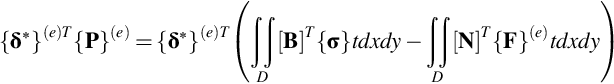
In order to make differentiations shown in Eq. (1.57), displacements assumed by Eq. (1.71) must be continuous everywhere in an elastic body of interest. The remaining conditions to satisfy are the equations of equilibrium (1.56) and the mechanical boundary conditions (1.63); nevertheless, these equations generally cannot be satisfied in the strict sense. Hence, defining the equivalent nodal forces, for instance, (X_1e, Y_1e), (X_2e, Y_2e), and (X_3e, Y_3e) on the three nodal points of the eth element and determining these forces by the principle of the virtual work in order to satisfy the equilibrium and boundary conditions element by element. Namely, the principle of the virtual work to be satisfied for arbitrary virtual displacements {δ⁎}^(e) of the eth element is derived from Eq. (1.66) as

${\{δ^{*}\}}^{(e) T} {\{P\}}^{(e)} = \iint_{D} ({\{ɛ^{*}\}}^{T} \{δ\} - {\{f^{*}\}}^{T} {\{F\}}^{(e)}) tdxdy$

si114_e (1.77)

where

$\{ɛ^{*}\} = [B] {\{δ^{*}\}}^{(e)}$

(1.78)

$\{f^{*}\} = [N] {\{δ^{*}\}}^{(e)}$

(1.79)

Substitution of Eqs (1.78), (1.79) into Eq. (1.77) gives.

${\{δ^{*}\}}^{(e) T} {\{P\}}^{(e)} = {\{δ^{*}\}}^{(e) T} (\iint_{D} {[B]}^{T} \{σ\} tdxdy - \iint_{D} {[N]}^{T} {\{F\}}^{(e)} tdxdy)$

si117_e (1.80)

Since Eq. (1.80) holds true for any virtual displacements {δ⁎}^(e), the equivalent nodal forces can be obtained by the following equation:

${\{P\}}^{(e)} = \iint_{D} {[B]}^{T} \{σ\} tdxdy - \iint_{D} {[N]}^{T} {\{F\}}^{(e)} tdxdy$

si118_e (1.81)

From Eqs (1.73), (1.74),

$\{σ\} = [D^{e}] (\{ɛ\} - \{ɛ_{0}\}) = [D^{e}] [B] {\{δ\}}^{(e)} - [D^{e}] \{ɛ_{0}\}$

(1.82)

Substitution of Eq. (1.82) into Eq. (1.81) gives

${\{P\}}^{(e)} = (\iint_{D} {[B]}^{T} [D^{e}] [B] tdxdy) {\{δ\}}^{(e)} - \iint_{D} {[B]}^{T} [D^{e}] \{ɛ_{0}\} tdxdy - \iint_{D} {[N]}^{T} {\{F\}}^{(e)} tdxdy$

si120_e (1.83)

Eq. (1.83) is rewritten in the form

${\{P\}}^{(e)} = [k^{(e)}] {\{δ\}}^{(e)} + {\{F_{ɛ_{0}}\}}^{(e)} + {\{F_{F}\}}^{(e)}$

(1.84)

where

$[k^{(e)}] \equiv \iint_{D} {[B]}^{T} [D^{e}] [B] tdxdy = Δ^{(e)} {[B]}^{T} [D^{e}] [B] t$

si122_e (1.85)

${\{F_{ɛ_{0}}\}}^{(e)} \equiv - \iint_{D} {[B]}^{T} [D^{e}] \{ɛ_{0}\} tdxdy$

si123_e (1.86)

${\{F_{F}\}}^{(e)} \equiv - \iint_{D} {[N]}^{T} {\{F\}}^{(e)} tdxdy$

si124_e (1.87)

Eq. (1.84) is called the element stiffness equation for the eth triangular finite element and [k^(e)] defined by Eq. (1.85) the element stiffness matrix. Since the matrices [B] and [D^e] are constant throughout the element, they can be taken out of the integral and the integral is simply equal to the area of the element Δ^(e) so that the rightmost side of Eq. (1.85) is obtained. The forces {F_ɛ₀}^(e) and {F_F}^(e) are the equivalent nodal forces due to initial strains and to body forces, respectively. Since the integrand in Eq. (1.85) is generally a function of the coordinate variables x and y except for the case of three-node triangular elements, the integrals appearing in Eq. (1.85) are often evaluated by numerical integration scheme such as the Gaussian quadrature.

The element stiffness matrix [k^(e)] in Eq. (1.85) is a 6 × 6 square matrix which can be decomposed into nine 2 × 2 submatrices, as shown in the following equation:

$[k_{ieje}^{(e)}] = [\begin{array}{c} k_{1 e 1 e}^{(e)} & k_{1 e 2 e}^{(e)} & k_{1 e 3 e}^{(e)} \\ k_{2 e 1 e}^{(e)} & k_{2 e 2 e}^{(e)} & k_{2 e 3 e}^{(e)} \\ k_{3 e 1 e}^{(e)} & k_{3 e 2 e}^{(e)} & k_{3 e 3 e}^{(e)} \end{array}]$

si125_e (1.88)

$k_{ieje}^{(e)} = k_{jeie}^{(e) T}$

(1.89)

$k_{ieje}^{(e)} = \int_{Δ^{(e)}} {[B_{ie}]}^{T} [D^{e}] [B_{je}] tdxdy \{\begin{cases} (2 \times 2) asymmetric matrix (i_{e} \neq j_{e}) \\ (2 \times 2) symmetric matrix (i_{e} = j_{e}) \end{cases}$

si127_e (1.90)

where

$[B_{ie}] \equiv \frac{1}{2 Δ^{(e)}} [\begin{array}{c} b_{ie} & 0 \\ 0 & c_{ie} \\ c_{ie} & b_{ie} \end{array}] (i_{e} = 1, 2, 3)$

si128_e (1.91)

and the subscripts i_e and j_e of k_ieje^(e) refers to element nodal numbers, and

$k_{ieje}^{(e)} = {[B_{ie}]}^{T} [D^{e}] [B_{je}] t Δ^{(e)}$

(1.92)

In the above discussion, the formulae have been obtained for just one triangular element, but are available for any types of elements, if necessary, with some modifications.

1.4.4.4 Global stiffness equations

Element stiffness equations as shown in Eq. (1.84) are determined element by element, and then they are assembled into the global stiffness equations for the whole elastic body of interest. Since nodal points which belong to different elements but have the same coordinates are the same points, the following points during the assembly procedure of the global stiffness equations should be noted:

1. The displacement components u and v of the same nodal points which belong to different elements are the same; i.e. there exist no incompatibilities such as cracks between elements.
2. For nodal points on the bounding surfaces and for those in the interior of the elastic body to which no forces are applied, the sums of the nodal forces are to be zero.
3. Similarly, for nodal points to which forces are applied, the sums of the nodal forces are equal to the sums of the forces applied to those nodal points.

The same global nodal numbers are to be assigned to the nodal points which have the same coordinates. Taking the points described above into consideration, let us rewrite the element stiffness matrix [k^(e)] in Eq. (1.88) by using the global nodal numbers I, J and K (I, J, K = 1, 2, …, 2n) instead of the element nodal numbers i_e, j_e and k_e (i_e, j_e, k_e = 1, 2, 3); i.e.,

$[k^{(e)}] = [\begin{array}{c} k_{II}^{(e)} & k_{IJ}^{(e)} & k_{IK}^{(e)} \\ k_{JI}^{(e)} & k_{JJ}^{(e)} & k_{JK}^{(e)} \\ k_{KI}^{(e)} & k_{KJ}^{(e)} & k_{KK}^{(e)} \end{array}]$

si130_e (1.93)

Then, let us embed the element stiffness matrix in a square matrix having the same size as the global stiffness matrix of 2n × 2n, as shown in Eq. (1.94):

eq01-01-9780081021644 (1.94)

where n denotes the number of degrees of freedom. This procedure is called the method of extended matrix. The number of degrees of freedom here means the number of unknown variables. In two-dimensional elasticity problems, since two displacements and forces in the x- and y-directions are unknown variables for one nodal point, every nodal point has two degrees of freedom. Hence, the number of degrees of freedom for a finite element model consisting of n nodal points is 2n.

By summing up the element stiffness matrices for all the n_e elements in the finite element model, the global stiffness matrix [K] is obtained as shown in the following equation:

$[K] \equiv [K_{ij}] = \sum_{e = 1}^{ne} [K^{(e)}] (i j = 1 2 \dots 2 n and e = 1 2 \dots n_{e})$

si131_e (1.95)

Since the components of the global nodal displacement vector {δ} are common for all the elements, they remain unchanged during the assembly of the global stiffness equations. By rewriting the components of {δ}, u₁, u₂, …, u_n as u₁, u₃, …, u_2i − 1, …, u_2n − 1 and v₁, v₂, …, v_n as u₂, u₄, …, u_2i, …, u_2n, the following expression for the global nodal displacement vector {δ} is obtained:

$\{δ\} = {[u_{1}, u_{2}, \dots, u_{2 I - 1}, u_{2 I}, \dots, u_{2 J - 1}, u_{2 J}, \dots, u_{2 K - 1}, u_{2 K}, \dots, u_{2 n - 1}, u_{2 n}]}^{T}$

(1.96)

The global nodal force of a node is the sum of the nodal forces for all the elements to which the node belongs. Hence, the global nodal force vector {P} can be written as

$\{P\} = {[X_{1}, Y_{1}, \dots, X_{I}, Y_{I}, \dots, X_{J}, Y_{J}, \dots, X_{K}, Y_{K}, \dots, X_{n}, Y_{n}]}^{T}$

(1.97)

where

$X_{I} = \sum X_{I}^{(e)}, Y_{I} = \sum Y_{I}^{(e)} (I = 1 2 \dots n)$

(1.98)

By rewriting the global nodal force vector {P} in a similar way to {δ} in Eq. (1.96) as

$\{P\} = {[X_{1}, X_{2}, \dots, X_{2 I - 1}, X_{2 I}, \dots, X_{2 J - 1}, X_{2 J}, \dots, X_{2 K - 1}, X_{2 K}, \dots, X_{2 n - 1}, X_{2 n}]}^{T}$

(1.99)

where

$X_{I} = \sum X_{I}^{(e)} (I = 1 2 \dots 2 n)$

(1.100)

The symbol Σ in Eqs (1.98), (1.100) indicate that the summation is taken over all the elements that possess the node in common. The values of X_I in Eq. (1.100), however, are zero for the nodes inside of the elastic body and for those on the bounding surfaces which are subjected to no applied loads.

Consequently, the following formula is obtained as the governing global stiffness equation:

$[K] \{δ\} = \{P\}$

(1.101)

which is the 2nth degree simultaneous linear equations for 2n unknown variables of nodal displacements and/or forces.

..................Content has been hidden....................

You can't read the all page of ebook, please click here login for view all page.

Table of Contents for 1: Fundamentals of the finite element method

Create new playlist

Sign In

Sign Up

1.1 Method of weighted residuals

1.1.1 Subdomain method (finite volume method)

1.1.2 Galerkin method

1.2 Rayleigh–Ritz method

1.3 Finite element method

1.3.1 One-element case

1.3.2 Three-element case

1.4 FEM in two-dimensional elastostatic problems

1.4.1 Elements of finite-element procedures in the analysis of plane elastostatic problems

1.4.2 Fundamental formulae in plane elastostatic problems

1.4.2.1 Equations of equilibrium

1.4.2.2 Strain–displacement relations

1.4.2.3 Stress–strain relations (constitutive equations)

1.4.2.4 Boundary conditions

1.4.3 Variational formulae in elastostatic problems: The principle of virtual work

1.4.4 Formulation of the fundamental finite-element equations in plane elastostatic problems

1.4.4.1 Strain–displacement matrix or [B] matrix

1.4.4.2 Stress–strain matrix or [D] matrix

1.4.4.3 Element stiffness equations

1.4.4.4 Global stiffness equations

Table of Contents for
1: Fundamentals of the finite element method