3. The Origins of Asserted Versioning
Computer Science Research
We begin this chapter with an overview of the three sources of Asserted Versioning: computer science work on temporal data; best practices in the IT profession related to versioning; and original work by the authors themselves. We then spend the rest of this chapter discussing computer science contributions to temporal data management, and the relevance of some of these concepts to Asserted Versioning.
The Roots of Asserted Versioning
Over the last three decades, the computer science community has done extensive work on temporal data, and especially on bi-temporal data. During that same period of time, the IT community has developed various forms of versioning, all of which are methods of managing one of the two kinds of uni-temporal data.
Asserted Versioning may be thought of as a method of managing both uni- and bi-temporal data which, unlike the standard model of temporal data management, recognizes that rows in bi-temporal tables represent versions of things and that, consequently, these rows do not stand alone as semantic objects. Versions that are versions of the same thing are related to one another by that very fact. Versions that are versions of the same thing, and also that together represent an unbroken period of time in the life of that thing, are even more closely related to one another. Groups of temporally contiguous versions of the same thing are semantic objects that must be managed as single temporal objects, even though they may consist of any number of physical rows. These single semantic objects are what we call episodes.
Asserted Versioning may also be thought of as a form of versioning, a technique for managing historical data that has evolved in the IT industry over the last quarter-century. But unlike existing best practice variations on that theme, Asserted Versioning supports the full semantics of versions, i.e. everything that it is conceptually possible to do with versions. In addition, Asserted Versioning also integrates the management of versions with the management of assertions and with the management of bi-temporal data. As we pointed out earlier, it directly manages bi-temporal physical tables, and manages both forms of uni-temporal tables, as well as conventional tables, as views over those bi-temporal tables.
Besides embracing contributions from computer science research and from business IT best practices, we believe that Asserted Versioning introduces three new concepts to the field of temporal data management. The first concept is that of an episode. In making episodes central to its management of temporal data, Asserted Versioning breaks with a basic component of the relational model, which is that integrity constraints apply only to individual rows. For example, referential integrity, in the relational model, requires that every foreign key in one row expresses a valid relationship which that row has to one other row. In Asserted Versioning, a temporalized foreign key expresses a relationship which one row, called a version, has to an episode, not to any single row which is part of that episode.
The second concept is that of the internalization of pipeline datasets. We define a pipeline dataset as any collection of business data that is not a production table, but that contains data whose destination or origin is such a table. 1 Pipeline datasets which contains data destined for production tables are inflow pipeline datasets. Pipeline datasets which contain data derived from production tables are outflow pipeline datasets.
1The term “production” indicates that these tables contain “real” data. Regularly scheduled processes are being carried out to maintain these tables, and to keep their contents as accurate, secure and current as possible. Regularly scheduled processes, as well as non-scheduled ones, are being carried out to access this data to obtain needed information. So production tables are the tables that the business tries to keep accurate, current and secure, and from which it draws the information it needs to carry out its mission and meet its objectives.
History tables are one example of a pipeline dataset. Sets of transactions, accumulated in files or tables and waiting to be applied to their target tables, are another example. While the use of versions eliminates history tables by internalizing them within the tables whose history they track, the use of deferred transactions and deferred assertions eliminates batch files of transactions waiting to be applied to a database by also internalizing them within their target tables. In this book, we will show how the use of these internalized managed objects reduces the costs of maintaining databases by replacing external files or tables such as history tables, transaction files and logfiles, with structures internalized within production tables rather than being external to them.
The third concept is that of encapsulation, as it applies to the management of temporal data. Asserted Versioning fully encapsulates the complexities of maintaining temporal tables by distinguishing between temporal transactions and physical transactions. Temporal transactions are inserts, updates and deletes, as written by their authors, whose targets are asserted version tables. They are submitted to the Asserted Versioning Framework (AVF), not directly to the DBMS. The AVF translates them into physical insert and update transactions which it submits to the DBMS. These physical transactions implement the intentions expressed in those temporal transactions, and we note that, except for temporal insert transactions, one temporal transaction will always be translated into multiple physical transactions. In Part 3, we discuss several temporal transactions, and show both the physical transactions the AVF creates to implement these temporal transactions, and also how the AVF knows how to map between the two.
The practical orientation of Asserted Versioning is manifest in its encapsulation of the complexities of temporal data structures and the processes that manage them. Asserted Versioning is an integrated method of managing temporal data which relieves data modelers of the burden of designing and maintaining data models that must explicitly define temporal data structures and integrity constraints on them. It also relieves developers of the burden of designing, writing and maintaining code that enforces the rules which provide the semantics of temporal data. And it relieves query authors, whether developers or end users, of the burden of writing complex queries that must explicitly check for temporal gaps or overlaps, along one or two temporal dimensions, among a set of rows accessed by the query.
The origins of Asserted Versioning in computer science research, in IT best practices, and in contributions from the authors, are illustrated in Figure 3.1. Although deferred transactions and deferred assertions are the mechanisms for the internalization of several pipeline datasets, they are shown as a separate item in Figure 3.1 because of their particular importance.
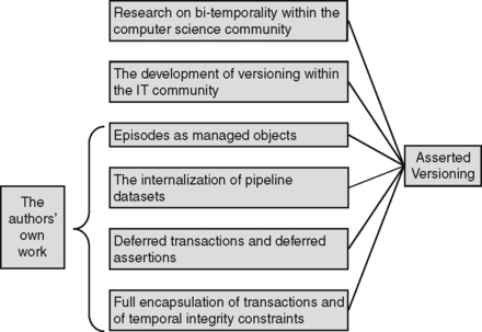 |
| Figure 3.1 The Origins of Asserted Versioning. |
Computer Science Research
In 2000, Dr. Rick Snodgrass stated that academics had published, at that time, over 1500 articles on temporal data management [2000, Snodgrass, xviii]. And over the last decade, much additional work has been done. For our purposes, this work falls into two categories: (i) research relevant to our task of designing and building a method of temporal data management that works with today's technology; and (ii) research on future directions for the implementation of temporal functions in commercial DBMSs, and for the specification of these functions in extensions to the current SQL standard.
Clocks and Clock Ticks
An atomic clock tick is the smallest interval of time recognized by the DBMS that can elapse between any two physical modifications to a database. 2 We note that the standard computer science term for an atomic clock tick is a chronon. A clock tick is an interval of time defined on the basis of atomic clock ticks, and that is used in an Asserted Versioning database to delimit the two time periods of rows in asserted version tables, and also to indicate several important points in time. In asserted version tables, clock ticks are used for effective time begin and end dates and for episode begin dates; and atomic clock ticks are used for assertion time begin and end dates, and for row create dates.
2We are not referring here to the cesium-based atomic clock on which standard time is based. An atomic clock tick, in the sense being defined here, is a logical concept, not a physical one.
Clock ticks may be defined at any level of granularity supported by the underlying DBMS. A timestamp is a typical clock tick. A date represents a daily clock tick. A 1-month clock tick represents a situation in which a database is updated from a collection of transactions at most once a month.
When time periods measured in clock ticks of different granularities are compared, the technical issues involved in the comparison are complex, even if the conceptual issues are not. In our own implementation of Asserted Versioning, we finesse these issues by requiring that all asserted version tables in the same database use clock ticks of the same granularity. In this book, we assume, albeit somewhat unrealistically, that all asserted version tables use a clock that ticks once a month (except where otherwise noted), and we will use the first day of each month to represent those clock ticks. This means that changes to these asserted version tables happen on the first of each month and, by the same token, that the state of the database after each monthly update will remain unaltered for the rest of the month.
But no matter what granularity we choose for our clock ticks, there is the issue of how clock ticks of one level of granularity are mapped onto those of another level. For example, if we choose a clock tick of one day, when does that day start? Does June 1st, 2012 begin at 2012-06-01-12:00:00.000, or perhaps at 2012-06-01-12:00:00.001, or perhaps even at 2012-05-31-11:59:59.999? The simplest solution is to let the DBMS determine the mapping for us; and in most cases this is perfectly adequate. But IT data management professionals should at least be aware that issues like these do exist.
They should also be aware that another issue exists, that of how SQL timestamps map to when things happen in the real world. SQL uses Universal Coordinated Time (UTC), which is based on cesium clocks, which might lead us to conclude that SQL timestamps are extremely accurate. Precise they may be; but issues of accuracy involved in their use do exist.
For example, suppose we know that an astronomical event which has just happened will happen again in exactly 725 days, 5 hours and 23 seconds. If we know the SQL timestamp when the event occurred, can we calculate exactly what the SQL timestamp will be when the event happens again? We can, of course, calculate the number of seconds that will have elapsed between the two events, that number being 62,658,023.
But it is a mistake to conclude that from knowing the timestamp of the first event and also knowing the number of seconds until the second event, we can calculate the timestamp of the second event. In fact, we cannot reliably do that. The reason is that from the moment the first timestamp is current to the moment that the second timestamp is current, one or more leap seconds may have been added to or subtracted from the count of cesium clock ticks between those two timestamps, and for the same reason that a leap day is added to the Gregorian calendar once every four years. But unlike the leap year adjustment, which is regular enough to count on, we do not know, in advance, how many leap seconds might be added or subtracted between now and the next occurrence of that astronomical event, or when those adjustments may occur.
The unpredictable adjustment of UTC and its SQL timestamps by means of leap seconds is seldom an issue in business IT. The reason is that for business purposes, we all tag our data with SQL timestamps, and we all regard those timestamps as an accurate record of when business events happen in the real world. In addition, for most business purposes, we assume that a SQL timestamp plus a defined interval of time will result in a second timestamp that represents when some second event will occur. 3
Time Periods and Date Pairs
SQL does not recognize a period of time as a managed object. Instead, we have to use a pair of dates. There are four ways we can use a pair of dates to do this. Either the beginning date, or the ending date, or both, may or may not be included in the time period they delimit. If a date is not included, the time period is said to be open on that end; otherwise it is said to be closed.
A discussion of all four ways of representing time periods with begin and end dates can be found in the book presenting the standard temporal model [2000, Snodgrass] and also in the book presenting the alternative temporal model [2002, Date, Darwen, Lorentzos]. Here, we discuss just two of the four combinations: closed-open and closed-closed. This is because the closed-open representation is actually the best way of representing time periods, whereas the closed-closed representation appears to be the best way of doing that.
Consider two versions of the same object, V1 and V2. In both cases, in this example, the first time period for the object starts on 2/19/2011 and ends on 5/22/2011, and the second starts on 5/23/2011 and ends on 10/14/2012. 4 Consequently there is no gap in time between these two time periods. 5/22/2011 and 5/23/2011 are contiguous clock ticks.
How are we to represent this? Two of the possibilities are shown in Figures 3.2 and 3.3.
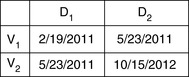 |
| Figure 3.2 A Closed-Open Representation of Two Time Periods. |
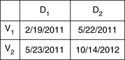 |
| Figure 3.3 A Closed-Closed Representation of Two Time Periods. |
Given that the first time period starts on 2/19/2011 and ends on 5/22/2011, and that the second time period starts on 5/23/2011 and ends on 10/14/2012, it might seem that the closed-closed representation is obviously the correct one, and that the closed-open representation is obviously wrong. But that is not the case.
If we wanted to argue in support of the closed-closed representation, we could try to show that the closed-open representation should not be used by querying for the time period that contains the date 5/23/2011. On the closed-open representation, it might seem that we can't tell to which version 5/23/2011 belongs. But in fact, we can. We just need the following WHERE clause predicate in our SQL query:
WHERE D1 <= ‘05/23/2011’ AND ‘05/23/2011’ < D2
With this predicate, the query will correctly pick out V2 from Figure 3.2.
So one reason we might have thought that the closed-closed representation is right is that its begin and end dates are the same dates we used to set up the example when we said that one period begins and ends on one set of dates and the other period begins and ends on the other set of dates. Another reason we might have thought that the closed-closed representation is right is that we are looking for a pair of dates that a third date is between.
Between, in one sense, is on display in the statement “Pick a number between 1 and 10”. We all know that 1 and 10 are both numbers that we can pick. And the SQL BETWEEN operator corresponds to this sense of the word. So if we use the closed-closed representation, we can write:
WHERE ‘05/23/2011’ BETWEEN D1 AND D2
In other words, when a closed-closed representation is used, we can rely on SQL's BETWEEN to express what we ordinarily mean by “between”, which is what we might call the inclusive sense of “between”.
But there is another sense of between, which is on display in the statement “The abandoned car is somewhere between mileposts 6 and 10, along I-65N, heading out of Pensacola”. We all know that to find the car, we should start at milepost 6 and continue up to milepost 10. In particular, we know that we don't need to search past milepost 10, i.e. past the start of the tenth mile heading out of Pensacola.
This is the sense of between used in the closed-open convention. The closest English equivalent would be “from . . . . . up to”, in the sense of “from” and then “up to but not including”. But since each SQL predicate returns the correct result, provided each is used with its corresponding method of representing periods of time, each method is correct.
What, then, is the advantage of using the closed-open representation? Well, look again at the two ways of representing V1 and V2. In both cases, V1 and V2 are contiguous. We know this because we have set up the example that way. And with the closed-open representation, we can immediately see that there is no gap between V1 and V2. But with the closed-closed representation, we don't know whether there is a gap or not. To make that determination, we also need to know at what rate the clock ticks. Assuming for this particular example that the clock ticks once a day, then only when given this additional information can we determine, from a closed-closed representation, that V1 and V2 have no gap between them.
This difficulty of determining whether or not two consecutive versions of the same object are contiguous is not just a problem for the human beings trying to understand the data. It is also a problem for the code which will often be called upon to determine, of two consecutive versions, whether or not they are contiguous, i.e. whether or not there is a clock tick between them. With a closed-open representation, the code only has to compare two values to see whether or not they are EQUAL.
Making matters worse, the granularity of DBMS timestamp datatypes has changed over time. Originally, these timestamps were seconds. Later, they were expressed as milliseconds, then partial microseconds, then microseconds, and now we are almost at the point where timestamps will be expressed in nanoseconds. With this sliding scale, across DBMSs and DBMS upgrades, we might not even know the granularity at which to try to determine if two versions are or are not contiguous. With a closed-open representation, the code to make this determination is trivial. With a closed-open representation, it may actually be impossible.
Once the SQL standards groups can agree on temporal extensions to the SQL standard, part of that agreement will certainly be a way of representing time periods directly, without relying on the confusing circumlocutions of various ways of using pairs of dates to represent time periods. But our concern, in this book, is with today's SQL, and so we must choose a date-pair method of representation. 5 Therefore, from this point forward, we will use the closed-open representation for time periods.
5Support for a PERIOD datatype has been introduced by such vendors as Oracle and Teradata. But what that support means may differ from vendor to vendor. Can a unique index be defined on a PERIOD datatype? Which of the Allen relationship comparisons are also supported? So, lacking a standard for the PERIOD datatype, we will continue the practice of defining periods of time in terms of their begin and end points in time.
9999 and 12/31/9999
We will use the notation 9999 in our illustrations, to represent the latest date that the DBMS can recognize and manipulate. That latest date cannot be used in effective or assertion begin dates. If it is used as business data, then it has whatever meaning its users assign to it, which will probably be as the designation of a day which is still a long way off. But if it is used in effective or assertion end dates, it is treated as a date by the DBMS but is not interpreted as a date by the users of the system. Instead, to those users, it means “later than now”. Equivalently, we can say that it means “end of the time period not known, but assumed to not have happened yet”. We will generally use the phrase until further notice to represent this semantics—in effect until further notice, or asserted as true until further notice.
When we specify an insert or an update against a conventional table, we normally do not know when, if ever, the target row will be next updated or deleted. By the same token, when we specify a temporal insert or a temporal update against a bi-temporal table, we normally do not know when, if ever, the effective time period of the new version will end, because we don't know when, if ever, a subsequent update or deletion will occur.
Some data modelers will argue that NULL should be used for unknown data. While logically, this is true, the performance of the physical model will benefit from this non-null datatype, as will be explained in Chapter 15. Moreover, we do know one thing about this unknown date. For as long as it is unknown, we choose to assume that it has not happened yet. In other words, for as long as it is unknown, we want the DBMS to tell us that it is greater than the value of Now(), whenever we ask that question. If we used NULL instead of a data value, the DBMS would not give us that answer to that question.
If an effective end date is unknown, then, instead of using NULL, we will set it to 12/31/9999, or to whatever value represents the future-most date that the particular DBMS can manage. So the semantics is date unknown (but still in the future), but the implementation is a real date, one in this case that is nearly 8000 years from now. How does a date like that represent semantics like that?
First, we assume that the date 12/31/9999 will not be required to represent that far-off New Year's Eve. So it is available to use for a special purpose. In the case of an effective end date, we often insert or update versions without knowing when the effective time period of the new version may end. So in this case, 12/31/9999 means that the end of the effective time period of the version thus marked is unknown, and that the time period will remain in effect until further notice. For example, when a customer's address is added to the database, we usually will not know when that customer will move from that address. So the status of that address is that it will remain in effect until that customer moves, at some unknown date in the future.
In the case of an assertion end date, that date is always set to 12/31/9999 when a row is created. This reflects the assumption that we would never want to assert that a version is true, while also knowing that, at some later point in time, we will change our minds and no longer be willing to make that assertion. While we adopt this assumption in this book, and in the software which is our implementation of these concepts, we note that a more robust semantics might not include this assumption and that, consequently, later releases of our Asserted Versioning Framework may permit non-12/31/9999 assertion end dates to be specified on temporal transactions. 6
6As we briefly allude to, later on, what we assert by means of a row in a table is not so much that the statement made by the row is true. It is, rather, that the statement is actionable. An actionable statement, roughly, is one which is good enough to base a business decision on. Presumably, statements about the past or the present must be true in order to be actionable. But statements about the future, such as financial forecasts, lack a known truth value until the future time about which they are forecasting comes to pass, at which point those statements become either true or false. Such statements may be actionable when first made, and thus be actionable without being true. Moreover, they may be actionable when first made but, over time, become outdated, even prior to becoming true or false. (See, later in this chapter, the section The Very Concept of Bi-Temporality. See also Chapter 13, the section Posted Projections: Past Claims About the Future.)
An effective end date may be changed, i.e. the time period it ends may be shortened or lengthened, as long as the change does not violate temporal integrity constraints, which we will discuss in Part 3. As for an assertion end date, it may be changed for one of four reasons.
First, an assertion end date may be changed because we realize that the assertion is incorrect, and we have the correction for that error. In that case, the incorrect assertion will cease to be asserted, i.e. it will be withdrawn, as part of the same atomic unit of work that inserts the correcting assertion, and the same date will be used both for the assertion end date of the incorrect assertion and the assertion begin date of the correcting assertion.
Second, an assertion end date may be changed because we realize that an assertion is incorrect even though we do not know what the correct data is, or else just because, for some reason, we do not wish to make that assertion any longer. Third, we may conclude that an assertion about the future is no longer actionable, probably because both we and our competitors have more recent and presumably more accurate forecasts. In either case, the row representing that assertion will cease to be asserted on that date even if no correcting assertion is supplied to replace it.
The last reason an assertion end date may be changed is to lock an assertion which has been updated or deleted by a deferred transaction, until the resulting deferred assertion becomes current. We will have more to say about deferred transactions, deferred assertions and locking in Chapter 13.
Now() and UTC
Keeping our notation DBMS agnostic, and keeping the clock tick granularity generic, we will refer to the current moment, to right now, as Now(). 7 SQL Server may use getdate(), and DB2 may use Current Timestamp or Current Date. Depending on our clock tick duration, we might need to use a date formatting function to set the current granularity. In our examples, we generally use one month as our clock tick granularity. However for our purposes, Now() can take on values at whatever level of granularity we choose to use, including day, second or microsecond.
7Now() is a function that returns the current date. It is not a value. However, we will often use it to designate a specific point in time. For example, we may say that a time period starts at Now() and continues on until 12/31/9999. This is a shorthand way of emphasizing that, whenever that time period was created, it was given as its begin date the value returned by Now() at that moment.
Now() is usually assumed to represent the current moment by using local time. But local time may change because of entering or leaving Daylight Savings Time. And another issue is time zone. At any one time, data about to update a database may exist in a different time zone than the database itself. Users about to retrieve data from a database may exist in a different time zone than the database itself. And, of course, federated queries may attempt to join data from databases located in different time zones.
So the data values returned by Now() can change for reasons other than the passage of time. Daylight Savings Time can change those values. At any one point in time, those values can differ because of time zones. Clearly, we need a reference framework, and a set of values, that will not change for any reason other than the passage of time, and that will be the same value, at any point in time, the world over and year around.
This reference framework is Universal Coordinated Time (UTC). 8 To make use of UTC, our Asserted Versioning Framework will convert local time to UTC on maintenance and queries, and will store Asserted Versioning temporal parameters, such as begin and end dates, in UTC. For example, with Policy_AV being an asserted version table of insurance policies, we would insert a policy like this:
INSERT INTO Policy_AV (oid, asr_beg_dt . . . . .)
VALUES (55, CURRENT TIMESTAMP - CURRENT TIMEZONE . . . . .)
8However, even in UTC, some variations in time values do not reflect the passage of time. We are referring here to the periodic adjustments in UTC made by adding or removing leap seconds, as we described in an earlier section of this chapter.
For queries, they will perform better if we do the time conversion before using the value as a selection predicate in the SQL itself. This is because most optimizers treat functions that appear in predicates as non-indexable. For example, in DB2, we should write:
SET :my-cut = TIMESTAMP(:my-local-time-value) - CURRENT TIMEZONE
SELECT . . . . . FROM . . . . .
WHERE oid = 55
AND asr_beg_dt <= :my-cut
AND asr_end_dt > :my-cut
rather than
SELECT . . . . . FROM . . . . .
WHERE oid = 55
AND asr_beg_dt <=
TIMESTAMP(:my-local-time-value) - CURRENT TIMEZONE
AND . . . . .
However, if these functions are used for display purposes, then there is no reason to exclude them from the queries. For example:
SELECT asr_beg_dt + CURRENT TIMEZONE AS my_local_asr_beg_dt . . . . . FROM . . . . .
It would also be useful to add alternate columns for the temporal dates in our views that have the translation to local time performed already.
The Very Concept of Bi-Temporality
Business IT professionals were using tables with both an effective date and a physical row create date by the early 90s. 9 But they were doing so with apparently no knowledge of academic work on bi-temporality. At that time, these version tables which also contained a row create date were state of the art in best practice methods for managing temporal data. We will discuss them in the next chapter.
9Or timestamps, or other datatypes. We remind the reader that, throughout this book, we use the date datatype for all temporal columns, and a first of the month value for all our dates. This simplifies the presentation without affecting any of the semantics. In real business applications, of course, these columns would often be timestamps.
With a row creation date, of course, any query can be restricted to the rows present in a table as of any specific date by including a WHERE clause predicate that qualifies only those rows whose create date is less than or equal to the specified date. With two effective dates, tables like these are also able to specify one of the two temporal dimensions that make up full bi-temporality.
The standard temporal model uses the term “valid time” where we use the term “effective time”. But the difference is purely verbal. We have found no differences between how valid time works in the standard model, and how effective time works in Asserted Versioning. We use “effective time” because it is the preferred term among business IT professionals, and also because it readily adapts itself to other grammatical forms such as “becoming effective” and “in effect”.
The standard model states that “(v)alid time … captur(es) the history of a changing reality, and transaction time . . . . . captur(es) the sequence of states of a changing table . . . . . A table supporting both is termed a “bi-temporal table” [2000, Snodgrass, p. 20]. But as we will see later, Asserted Versioning does not define bi-temporality in exactly the same way. The difference lies primarily in the second of the two temporal dimensions, what computer scientists call “transaction time” and what we call “assertion time”. While a transaction begin date always indicates when a row is physically inserted into a table, an assertion begin date indicates when we are first willing to assert, or claim, that a row is a true statement about the object it represents, during that row's effective (valid) time period, and also that the quality of the row's data is good enough to base business decisions on.
In the standard temporal model, the beginning of a transaction time period is the date on which the row is created. Obviously, once the row is created, that date cannot be changed. But in the Asserted Versioning temporal model, an assertion time period begins either on the date a row is created, or on a later date.
Because an assertion begin date is not necessarily the same as the date on which its row is physically created, Asserted Versioning needs, in addition to the pair of dates that define this time period, an additional date which is the physical creation date of each row. That date serves as an audit trail, and as a means of reconstructing a table as it physically existed at any past point in time.
What are these rows with future assertion begin dates? To take a single example, they might be rows for which we have some of the business data, but not all of it, rows which are in the process of being made ready “for prime time”. These rows—which may be assertions about past, present or future versions—are not yet ready, we will say, to become part of the production data in the table, not yet ready to become rows that we are willing to present to the world and of which we are willing to say “We stand behind the statements these rows make. We claim that the statements they make are (or are likely to become) true, and that the information these rows provide meets the standards of reliability understood (or explicitly stated) to apply to all rows in this table”.
So the semantics of the standard temporal model are fully supported by Asserted Versioning. But Asserted Versioning adds the semantics of what we call deferred assertions, and which we have just briefly described. As we will see in later chapters, deferred assertions are just one kind of internalized pipeline dataset, and the internalization of pipeline datasets can eliminate a large part of the IT maintenance budget by eliminating the need to manage pipeline datasets as distinct physical objects.
Allen Relationships
Allen relationships describe all possible positional relationships between two time periods along a common timeline. This includes the special case of one or both time periods being a point in time, i.e. being exactly one clock tick in length.
There are 13 Allen relationships in total. Six have a corresponding inverse relationship, and one does not. Standard treatments of the Allen relationships may be found in both [2000, Snodgrass] and [2002, Date, Darwen, Lorentzos]. We have found it useful to reconstruct the Allen relationships as a binary taxonomy. Our taxonomy is shown in Figure 3.4.
 |
| Figure 3.4 The Asserted Versioning Allen Relationship Taxonomy. |
In this diagram, the leaf nodes include a graphic in which there are two timelines, each represented by a dashed line. All the leaf nodes but one have an inverse, and that one is italicized; when two time periods are identical, they do not have a distinct inverse. Thus, this taxonomy specifies 13 leaf-node relationships which are, in fact, precisely the 13 Allen relationships.
The names of the Allen relationships are standard, and have been since Allen wrote his seminal article in 1983. But those names, and the names of the higher-level nodes in our own taxonomy of the Allen relationships, are also expressions in ordinary language. In order to distinguish between the ordinary language and the technical uses of these terms, we will include the names of Allen relationships and our other taxonomy nodes in brackets when we are discussing them. We will also underline the non-leaf node relationships in the taxonomy, to emphasize that they are relationships we have defined, and are not one of the Allen relationships.
In the following discussion, the first time period in a pair of them is the one that is either earlier than the other, or not longer than the other.
Given two time periods on a common timeline, either they have at least one clock tick in common or they do not. If they do, we will say that they [intersect] one another. If they do not, we will say that they [exclude] one another.
If there is an [intersects] relationship between two time periods, then either one [fills] the other or each [overlaps] the other. If one time period [fills] another, then all its clock ticks are also in the time period it [fills], but not necessarily vice versa. If one time period [overlaps] another, then the latter also overlaps the former; but, being the later of the two time periods, we say that the latter time period has the inverse relationship, [overlaps−1]. In the overlaps cases, each has at least one clock tick that the other does not have, as well as having at least one clock tick that the other does have.
If two time periods [exclude] one another, then they do not share any clock ticks, and they are either non-contiguous or contiguous. If there is at least one clock tick between them, they are non-contiguous and we say that one is [before] the other. Otherwise they are contiguous and we say that one [meets] the other.
If one time period [fills] the other, then either they are [equal], or one [occupies] the other. If they are [equal], then neither has a clock tick that the other does not have. If one [occupies] the other, then all the clock ticks in the occupying time period are also in the occupied time period, but not vice versa.
If one time period [occupies] the other, then either they share an [aligns] relationship, or one occurs [during] the other. If they are aligned, then they either start on the same clock tick or end on the same clock tick, and we say that one either [starts] or [finishes] the other. Otherwise, one occurs [during] the other, beginning after the other and ending before it. Note that if two time periods are aligned, one cannot both [start] and [finish] the other because if it did, it would be [equal] to the other.
If one time period [starts] another, they both begin on the same clock tick. If one [finishes] the other, they both end on the same clock tick. If one time period [occupies] another, but they are not aligned, then one occurs [during] the other.
Now let's consider the special case in which one of the two time periods is a point in time, i.e. is exactly one clock tick in length, and the other one contains two or more clock ticks. This point in time may either [intersect] or [exclude] the time period. If the point in time [intersects] the time period, it also [fills] and [occupies] that time period. If it [aligns] with the time period, then it either [starts] the time period or [finishes] it. Otherwise, the point in time occurs [during] the time period. If the point in time [excludes] the time period, then either may be [before] the other, or they may [meet].
Finally, let's consider one more special case, that in which both the time periods are points in time. Those two points in time may be [equal], or one may be [before] the other, or they may [meet]. There are no other Allen relationships possible for them.
As we will see later, four of these Allen relationship categories are especially important. They will be discussed in later chapters, but we choose to mention them here.
(i) The [intersects] relationship is important because for a temporal insert transaction to be valid, its effective time period cannot intersect that of any episode for the same object which is already in the target table. By the same token, for a temporal update or delete transaction to be valid, the target table must already contain at least one episode for the same object whose effective time period does [intersect] the time period designated by the transaction.
(ii) The [fills] relationship is important because violations of the temporal analog of referential integrity always involve the failure of a child time period to [fill] a parent time period. We will be frequently discussing this relationship from the parent side, and we would like to avoid having to say things like “. . . . . failure of a parent time period to be filled by a child time period”. So we will use the term “includes” as a synonym for “is filled by”, i.e. as a synonym for [fills−1]. Now we can say “. . . . . failure of a parent time period to include a child time period”.
(iii) The [before] relationship is important because it distinguishes episodes from one another. Every episode of an object is non-contiguous with every other episode of the same object, and so for each pair of them, one of them must be [before] the other.
(iv) The [meets] relationship is important because it groups versions for the same object into episodes. A series of versions for the same object that are all contiguous, i.e. that all [meet], fall within the same episode of that object.
Advanced Indexing Strategies
Indexes are one way to improve performance. And it should be clear that it would be a serious performance handicap if we could not define indexes over either or both of the two time periods of a bi-temporal table. But this proves to be more complex than it might at first sight appear to be.
The issue is that traditional indexes contain pointers to rows, pointers which are based on discrete values, while the two time periods of rows in bi-temporal tables are not discrete values, but rather an unbroken and non-overlapping sequence of such values. Such rows occupy points in effective (valid) time or in assertion (transaction) time only as a limit case. What they really occupy are intervals along those two timelines. That's the reason we need two dates to describe each of them. Traditional balanced-tree indexes work well with discrete values, including such discrete values as dates. But they don't work well with intervals of time, i.e. with time periods.
But indexing methods which manage intervals are being developed. Specifically, some bi-temporal indexing methods manage the two intervals for a bi-temporal object as a single unit, which would appear as a rectangle on a Cartesian graph in which one temporal dimension is represented by the X-axis and the other by the Y-axis.
Another approach is to manage each of the two temporal dimensions separately. One reason for taking this approach is that, for the standard temporal model, the two temporal dimensions behave differently. Specifically, for the standard model, transaction time always moves forwards, whereas valid time can move forwards or backwards. This means that a bi-temporal row can be inserted into a table proactively in valid time, but can never be inserted into a table proactively in transaction time.
Asserted Versioning, as we have already pointed out, supports both forwards and backwards movement in both temporal dimensions. So for Asserted Versioning, there is no difference in behavior which would justify separating the two temporal dimensions for indexing purposes. Specifically, Asserted Versioning supports both proactive (future-dated) versions and proactive assertions (i.e. deferred assertions) and also both retroactive versions and an approval transaction which can move deferred assertions backwards in time, but not prior to Now(). In Chapter 15, we will describe certain indexing strategies that will improve performance using today's DBMS index designs.
Temporal Extensions to SQL
Following [2000, Snodgrass], we will refer to a future release of the SQL language that will contain temporal extensions as SQL3. A more detailed discussion may be found in that book, although we should note that the book is, at the time of publication of this book, 10 years old.
Temporal Upward Compatibility
One issue related to changes in the SQL standard is temporal upward compatibility. In describing SQL3, Snodgrass states that “(t)emporal upward compatibility at its core says this: ‘Take an application that doesn't involve time, that concerns only the current reality . . . . . Alter one or more of the tables so that they now have temporal support . . . . . The application should run as before, without changing a single line of code’” [2000, Snodgrass, p. 449].
This cannot be an objective for Asserted Versioning, because we are limited to current SQL, not to a future release of SQL that builds temporal extensions into the language itself. But we can come close. We can achieve this objective for queries by using a view which filters out all but current data, and by redirecting existing queries to that view. We can achieve this objective for temporal inserts, updates and deletes by defining default effective and assertion dates for these transactions. These will be default dates that cause these transactions, as written by their authors, and as parsed and submitted to the DBMS by the AVF, to physically insert and update current assertions of the current versions of the objects they reference.
The PERIOD Datatype
A second issue related to changes in the SQL standard is the need for a PERIOD datatype. This new datatype will not change the semantics of temporal data management, but it will simplify the expression of those semantics. For one thing, a single column will replace a pair of dates. This will simplify the way that Allen relationships are specified in SQL statements. For example, it will change the expression with which we ask whether a point in time is or is not contained in a period of time. Where P and T are, respectively, a point in time and a period of time, and T1 and T2 are dates delimiting T using the closed-open representation, we currently must ask whether P is a clock tick within T like this:
WHERE T1 <= P AND P < T2
With the PERIOD datatype, and the new Allen relationship operators that will accompany it (including such derivative operators as those used in our taxonomy), we will be able to ask the same question like this:
WHERE T OCCUPIES P
A PERIOD datatype will also make it easier to enforce constraints on time periods, such as insuring that two time periods do not intersect. When representing time periods by means of begin and end dates, this is impossible to do with only an index. Here's why.
Consider the time period represented by the closed-open pair [4/23/2012 – 8/04/2014]. Suppose that we want to define an exclusive index on time periods. The problem is that there is no way, by means of any standards-compliant indexing method available with today's technology, to exclude [3/12/2011 – 4/24/2012], or [10/15/2012 – 9/30/2013], or [6/1/2014 – 12/31/2014], or any other time period that in fact [intersects] the time period designated by [4/23/2012 – 8/04/2014]. The index sees two columns of values, and knows that the combination of values must be unique in each instance. That's all it sees, that's all it knows, and that's all it can enforce.
But if we had a PERIOD datatype, and SQL extensions and indexing methods that could recognize and manage that datatype, then all the Allen relationships among time periods could be easily expressed, and the very important [excludes] relationship could be enforced by means of a unique index. Lacking that future technology, and the standards needed to insure interoperability across different vendor implementations, the AVF contains its own code that effectively turns pairs of dates into a user-defined PERIOD datatype.
Temporal Primary Keys
A third issue related to changes in the SQL standard is support for temporal primary keys. With those temporal extensions, we will be able to declare a temporal primary key to the DBMS and, by the same token, declare temporal foreign keys as well. But what is it we will be declaring? Temporal tags added to physically unique identifiers of rows of otherwise non-temporal tables? Or something more?
If a SQL standard for bi-temporality, when we eventually have one, is a standard for adding two temporal tags to rows in otherwise non-temporal tables, and providing a PERIOD data type and Allen relationship operators to manage the data thus tagged, then most of the semantics of bi-temporality will have been left out of that standard, and left up to developers. The managed objects of temporal data management are not physical rows in physical tables. They are collections of one or more rows which represent temporally delimited claims about temporally delimited statements about what real-world persistent objects were like, are like, or will be like.
As long as every database table contains one and only one row for each instance of the type indicated by the table, it is easy to forget about the semantics and concentrate on the mechanics. Primary key uniqueness is mechanics; its role in eliminating row-level synonyms—and its failure to address the problem of row-level homonyms—is the semantics that are easily and almost always overlooked. Foreign key referential integrity is mechanics; its role in expressing existence dependencies among the objects represented by those rows is the semantics that are easily and almost always overlooked.
It has been this one-to-one correlation between rows and the objects they represent that has made it easy to give short shrift to semantics, and to then get right down to what really fascinates engineering types—the mechanics of making things work. But once we attempt to manage both the epistemological and the ontological temporal dimensions of data, i.e. both assertion time and effective time, we must give up this comfortable one-to-one correlation. We must recognize that rows are no longer an adequate representation of the semantic objects that the bi-temporality of data reveals to us.
From the point of view of the conceptual foundations of Asserted Versioning, the declaration of a bi-temporal primary key must specify (i) a unique identifier for an object, (ii) an assertion time period, and (iii) an effective time period. In particular, that declaration must not specify simply (i) a unique identifier for an otherwise non-temporal row, (ii) a valid time period, and (iii) a transaction time period, one whose begin date is always the date on which the row was physically created.
Temporal Logic
A fourth issue related to changes in the SQL standard is temporal logic. SQL implements a subset of propositional and first-order predicate logic (FOPL). Temporal extensions to SQL are not a matter of simply adding temporal features to SQL until we're pleased with the result. The logical foundations of those temporal extensions must be explored so that, as SQL is extended, we can remain confident that it is logically sound. Examples of work in temporal logic include first-order temporal logic (FOTL). Just as FOPL uses the quantifiers for all X and for some X, FOTL adds the quantifiers at some time in the past, at every time in the past, at some time in the future and at every time in the future, and also adds the binary predicates SINCE and UNTIL.
Glossary References
Glossary entries whose definitions form strong inter-dependencies are grouped together in the following list. The same glossary entries may be grouped together in different ways at the end of different chapters, each grouping reflecting the semantic perspective of each chapter. There will usually be several other, and often many other, glossary entries that are not included in the list, and we recommend that the Glossary be consulted whenever an unfamiliar term is encountered.
We note, in particular, that none of the nodes in our Allen relationships taxonomy are included in this list. In general, we leave taxonomy nodes out of these lists, but recommend that the reader look them up in the Glossary.
clock tick
granularity
PERIOD datatype
point in time
time period
episode
managed object
object
pipeline dataset
inflow pipeline dataset
internalization of pipeline datasets
outflow pipeline dataset
replace
supercede
withdraw
statement
..................Content has been hidden....................
You can't read the all page of ebook, please click here login for view all page.