
4. Data and Methods in Data Mining
The popularity of data mining can be attributed to its ability to discover hidden patterns deep inside large data repositories that organizations are automatically accumulating these days. Data by itself is not valuable to organizations that are desperately looking for ways to make evidence-based intelligent decisions. It is only after methods are applied to data that the invaluable knowledge organizations need can be brought out. A large variety of methods and algorithms can be used to carry out different types of data mining tasks. Each of these methods has advantages and disadvantages for a given project, depending on the specific characteristics of the problem being addressed and the data set being used. Identifying the best method to use usually requires quite a bit of experimentation and sound comparative assessment.
This chapter provides rather detailed yet nontechnical descriptions of these methods and commonly applied assessment techniques. Before we get to that, though we need to first talk about data as it relates to data mining.
The Nature of Data in Data Mining
Data refers to a collection of facts usually obtained as a result of experiences, observations, or experiments. Data may consist of numbers, letters, words, images, voice recordings, and other variables. Data is often viewed as the lowest level of abstraction from which information and then knowledge are derived.
At the highest level of abstraction, one can classify data as structured and unstructured (or semi-structured). Unstructured/semi-structured data is composed of any combination of textual, imagery, voice, and Web content. Unstructured/semi-structured is covered in more detail in Chapter 6, “Text Analytics and Sentiment Analysis.” Structured data is the data that data mining algorithms uses, and it can be classified as categorical or numeric. Categorical data can be subdivided into nominal or ordinal data, whereas numeric data can be subdivided into interval or ratio data. Figure 4.1 shows a simple taxonomy of data as it relates to data mining.
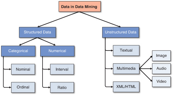
Categorical data falls into multiple classes used to divide a variable into specific groups. Examples of categorical variables include race, sex, age group, and educational level. Although age group and educational level may also be considered in a numerical manner by using exact values for age and highest grade completed, it is often more informative to categorize such variables into a relatively small number of ordered classes. The categorical data may also be called discrete data, implying that it represents a finite number of values with no continuum between them. Even if the values used for the categorical (or discrete) variables are numeric, these numbers are nothing more than symbols and do not imply the possibility of calculating fractional values.
Nominal data includes measurements of simple codes assigned to objects as labels, which are not measurements. For example, the variable marital status can be generally categorized as (1) single, (2) married, or (3) divorced. Nominal data can be represented with binomial values having two possible values (e.g., yes/no, true/false, good/bad), or multinomial values having three or more possible values (e.g., brown/green/blue, white/black/Latino/Asian, single/married/divorced).
Ordinal data includes codes assigned to objects or events as labels that also represent the rank order among them. For example, the variable credit score can be generally categorized as (1) low, (2) medium, or (3) high. Similar ordered relationships can be seen in variables such as age group (i.e., child/young/middle-aged/elderly) and educational level (i.e., high school/college/graduate school). Some data mining algorithms, such as ordinal multiple logistic regression, take into account this additional rank order information to build a better classification model.
Numeric data represents the numeric values of specific variables. Examples of numerically valued variables include age, number of children, total household income (in U.S. dollars), travel distance (in miles), and temperature (in Fahrenheit degrees). Numeric values representing a variable can be integer (taking only whole numbers) or real (taking also the fractional number). Numeric data may also be called continuous data, implying that the variable contains continuous measures on a specific scale that allows insertion of interim values. Unlike a discrete variable, which represents finite, countable data, a continuous variable represents scalable measurements, and it is possible for the data to contain an infinite number of fractional values.
Interval data includes variables that can be measured on interval scales. A common example of interval scale measurement is temperature on the Celsius scale. In this particular scale, the unit of measurement is 1/100 of the difference between the melting temperature and the boiling temperature of water in atmospheric pressure; that is, there is not an absolute zero value.
Ratio data includes measurement variables commonly found in the physical sciences and engineering. Mass, length, time, plane angle, energy, and electric charge are examples of physical measures that are ratio data. The scale type takes its name from the fact that measurement is the estimation of the ratio between a magnitude of a continuous quantity and a unit magnitude of the same kind. Informally, the distinguishing feature of a ratio scale is the possession of a nonarbitrary zero value. For example, the Kelvin temperature scale has a nonarbitrary zero point of absolute zero, which is equal to –273.15 degrees Celsius. This zero point is nonarbitrary because the particles that comprise matter at this temperature have zero kinetic energy.
Other data types, including textual, multimedia (e.g., image, audio, video), and XML/HTML need to be converted into some form of categorical or numeric representation before they can be processed by data mining algorithms. (For more details about how to mine knowledge from unstructured and semi-structured data, see Chapter 6.) Data can also be geographically oriented, so that the numeric and nominal data is enriched with locational/geographic information; this is often referred to as spatial data. Furthermore, regardless of its structure, data can also be classified as static or dynamic (i.e., temporal or time-series), based on its relationship to time.
Some data mining methods and algorithms are very particular about the type of data they can handle. Providing them with incompatible data types may lead to incorrect models or (more often) halt the model development process. For example, some data mining methods (e.g., neural networks, support vector machines, logistic regression) need all the variables (both input and output) represented as numerically valued variables. The nominal or ordinal variables are converted into numeric representations using some type of 1-of-N pseudo variables (e.g., a categorical variable with three unique values may be transformed into three pseudo variables with binary values—1 or 0). Because this process may increase the number of variables, one should be cautious about the effect of such representations, especially for the categorical variables that have large numbers of unique values.
Similarly, some data mining methods, such as ID3 (a classic decision tree algorithm) and rough sets (a relatively new rule-induction algorithm), need all the variables represented as categorically valued variables. Early versions of these methods required the user to discretize numeric variables into categorical representations before processing them with the algorithm. The good news is that most implementations of these algorithms in widely available software tools accept a mix of numeric and nominal variables and internally make the necessary conversions before processing the data.
Preprocessing of Data for Data Mining
The quality and usefulness of models created using data mining methods depends largely on the quality of the data used to build them. In that sense, perhaps the GIGO rule (i.e., garbage-in, garbage-out) is more applicable to data mining than to any other application domain. Therefore, the purpose of data preparation (or more commonly called data preprocessing) is to eliminate the possibility of GIGO errors by methodically cleaning and transforming data into a standard form so that it can be properly analyzed by appropriate data mining methods. Compared to the other activities in the data mining process, data preprocessing demands and consumes the most time and effort, often accounting for more than 80% of the total time spent on a project. Preprocessing requires such an enormous effort because real-world data is generally incomplete (lacking attribute values, lacking certain attributes of interest, or containing only aggregate data), dirty/noisy (containing errors or outliers), and inconsistent (containing discrepancies in codes or names). Therefore, diligent effort is necessary to clean and transform the data into a form that can be mined while making sure that the preprocessing does not bias the data; it is important to preserve the inherent patterns and relationships of the data. Figure 4.2 shows the four-step systematic process commonly followed to convert the raw real-world data into well-formed data sets that can be mined.

In the first phase of data preprocessing, the relevant data is collected from the identified sources, the necessary records and variables are selected (filtering out the unnecessary data, based on an intimate understanding of the data), and the records coming from multiple data sources are integrated. During this phase, domain-specific understanding of the data is applied to properly handle the synonyms and homonyms in the data.
In the second phase of data preprocessing, known as data scrubbing, the data is cleaned. In this step, the values in the data set are identified and dealt with. In some cases, missing values are an anomaly in the data set, in which case they need to be imputed (i.e., filled with a most probable value) or ignored; in other cases, the missing values are a natural part of the data set (e.g., the household income field is often left unanswered by people who are in the top income tier). In this step, the analyst should also identify noisy values in the data (i.e., outliers) and smooth them out. In addition, inconsistencies (unusual values within a variable) in the data should be handled using domain knowledge and/or expert opinion.
In the third phase of data preprocessing, the data is transformed for better processing. For instance, in many cases, data is normalized between a certain minimum and maximum for all variables in order to mitigate the potential bias of one variable dominating other variables having smaller values; for example, the analyst would not want data with large numeric values, such as for household income, to dominate the number of dependents or years in service, which may potentially be more important. Another transformation that takes place at this point is discretization and/or aggregation. In some cases, the numeric variables are converted to categorical values (e.g., low, medium, high); in other cases, a nominal variable’s unique value range is reduced to a smaller set, using concept hierarchies (e.g., instead of using the individual states with 50 different values, using several regions for a variable that shows location) in order to have a data set that is more amenable to computer processing. In yet other cases, one might choose to create new variables based on the existing ones in order to magnify the information found in a collection of variables in the data set. For instance, in an organ transplantation data set, an analyst might choose to use a single variable showing the blood type match (1: match, 0: no match) as opposed to using separate multinomial values for the blood types of the donor and the recipient. Such simplification may increase the information content while reducing the complexity of the relationships in the data.
The final phase of data preprocessing is data reduction. Data miners like to have large data sets, but too much data can be a problem. In the simplest sense, one can visualize the data commonly used in data mining projects as a flat file consisting of two dimensions: variables (the number of columns) and cases/records (the number of rows). In some cases (e.g., image processing, genome projects with complex microarray data), the number of variables can be rather large, and the analyst must reduce the number down to a manageable size. Because the variables are treated as different dimensions that describe the phenomenon from different perspectives, in data mining, this process is commonly called dimensional reduction. Even though there is not a single best way to accomplish this task, an analyst can use the findings from previously published literature, consult domain experts, run appropriate statistical tests (e.g., principal component analysis, independent component analysis), or, ideally, use a combination of these techniques to successfully reduce the dimensions in the data into a more manageable and relevant subset.
In addition to the complications related to multidimensionality, real-world data may also have issues with very large numbers of samples. That is, some data sets may include millions or billions of records (also called samples or cases). Even though computing power is increasing steadily, providing more horsepower for data analysis, processing such a large number of records may still not be feasible or practical; a single analysis may take a prohibitively long time to complete. In such cases, an analyst may need to analyze only a subset of the data. The underlying assumption of sampling is that the subset of the data will contain all relevant patterns of the complete data set. In a homogenous data set, such an assumption may hold well, but real-world data is hardly ever homogenous. The analyst should be extremely careful in selecting a subset of the data that reflects the essence of the complete data set and is not specific to a subgroup or subcategory. The data is usually sorted on some variable, and taking a section of the data from the top or bottom may lead to a biased data set on specific values of the indexed variable; therefore, one should always try to randomly select the records on the sample set. For skewed data, straightforward random sampling may not be sufficient, and stratified sampling—in which a proportional representation of different subgroups in the data is represented in the sample data set—may be required. In addition, it is a good practice to balance highly skewed data by either oversampling the less represented classes or undersampling the more represented classes. Research has shown that balanced data sets tends to produce better prediction models than unbalanced ones.
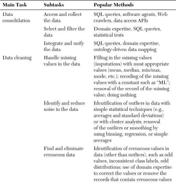
The process shown in Figure 4.2 is not a simple unidirectional, one-pass (top-to-bottom) effort. Rather, it is an iterative process that usually requires going backward (following the feedback loops) to make corrections and adjustments. The quality of outcomes (i.e., how well-formed the data ends up being) depends on the meticulous execution of this highly repetitive process between the later and earlier phases. The core activities in data preprocessing are summarized in Table 4.1, which maps the main tasks (along with their problem descriptions) to a representative list of methods and algorithms.

Data Mining Methods
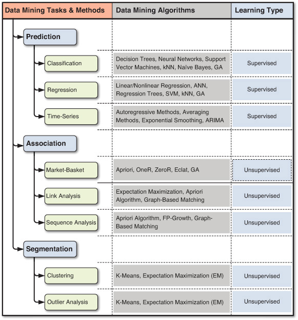
A wide variety of data mining methods and algorithms are being developed and used by businesses and scientific organizations to shed light on a range of complex problems. These problems can be mapped to a few high-level data mining tasks. Depending on the need and the nature of the problem, the data mining task can be classified as prediction (either classification or regression), association, or clustering. Each of these data mining tasks can use a variety of data mining methods and algorithms. Figure 4.3 shows a graphical representation of these data mining tasks, methods, and algorithms. The following sections describe these broad categories of data mining tasks (i.e., prediction, association, and clustering) and the algorithms most commonly used with them (e.g., decision trees for prediction, Apriori algorithm for association, k-means for clustering). Chapter 5, “Data Mining Algorithms,” explains several other data mining algorithms, including k-nearest neighbor, artificial neural networks, support vector machines, linear regression, logistic regression, and time-series forecasting. Most data mining software tools employ more than one technique (or algorithm) for each of these data mining tasks/methods.
Prediction
As discussed in Chapter 1, “Introduction to Analytics,” prediction (or predictive analytics) is used to foresee the future and answer the question “What will happen?” Business planning and problem solving rely heavily on the estimation of the future occurrences. Predictive analytics (and underlying prediction modeling techniques) are the enablers of these estimates. Regardless of the modeling technique used to do the predictive modeling, the underlying assumption is that what we already know about the past (in terms of recorded transaction and events, in the form of historical data) is what we use to predict the future. We assume that the past will repeat itself in the future; if it doesn’t, then there is no way of predicting the future.
Based on what we are predicting, the method of prediction can be labeled as classification (if we are predicting a discrete outcome), regression (if we are predicting a numerical value), or time-series forecasting (if we are predicting the future projection of a time-dependent value series). For instance, predicting whether a stock will close up or down at the end of the day is considered a classification, predicting the value difference of the stock at the end of the day is considered a regression, and predicting tomorrow’s closing price of the stock based on the closing prices in the recent past is a time-series prediction. Even though they all are estimating the future value of the variable, the value type and the nature of the variable determine the classification of the prediction.
Classification
Classification is perhaps the most commonly used data mining method for real-world problems. As a popular member in the machine learning family of techniques, classification learns patterns from past data (a set of information—traits, variables, and features—on characteristics of the previously labeled items, objects, or events) in order to place new instances (with unknown labels) into their respective groups or classes. For example, one could use classification to predict whether the weather on a particular day will be “sunny,” “rainy,” or “cloudy.” Popular classification tasks include credit approval (i.e., good or bad credit risk), store location (e.g., good/moderate/bad), target marketing (e.g., likely customer/no hope), fraud detection (i.e., yes/no), and telecommunication (e.g., likely/not likely to turn to another phone company). If what is being predicted is a class label (e.g., “sunny,” “rainy,” or “cloudy”) the prediction problem is called a classification, whereas if it is a numeric value (e.g., temperature such as 68°F), the prediction problem is called a regression.
Even though clustering (another popular data mining method) can also be used to determine groups (or class memberships) of things, there is a significant difference between the two. Classification learns the function between the characteristics of things (i.e., independent variables) and their membership (i.e., output variable) through a supervised learning process where both types (input and output) of variables are presented to the algorithm; in clustering, the membership of the objects is learned through an unsupervised learning process where only the input variables are presented to the algorithm. Unlike classification, clustering does not have a supervising (or controlling) mechanism that enforces the learning process; instead, clustering algorithms use one or more heuristics (e.g., multidimensional distance measure) to discover natural groupings of objects.
The most common two-step methodology of classification-type prediction involves model development/training and model testing/deployment. In the model development phase, a collection of input data, including the actual class labels, is used. After a model has been trained, the model is tested against the holdout sample for accuracy assessment and eventually deployed for actual use, where it predicts classes of new data instances (where the class label is unknown). Several factors are considered in assessing the model, including the following:
• Classification accuracy. This is the model’s ability to correctly predict the class label of new or previously unseen data. Prediction accuracy is the most commonly used assessment factor for classification models. To compute this measure, actual class labels of a test data set are matched against the class labels predicted by the model. The accuracy can then be computed as the accuracy rate, which is the percentage of test data set samples correctly classified by the model. (More on this topic is provided later in the chapter.)
• Speed. Speed is the computational cost involved in generating and using the model, where faster is deemed to be better.
• Robustness. Robustness refers to a model’s ability to make reasonably accurate predictions, given noisy data or data with missing and erroneous values.
• Scalability. Scalability is the ability to construct a prediction model efficiently, given a rather large amount of data.
• Interpretability. Interpretability is the level of understanding and insight provided by the model (e.g., how and/or what the model concludes on certain predictions).
How to Estimate the True Accuracy of Classification Models
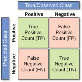
In classification problems, the primary source for accuracy estimation is a confusion matrix, also called a classification matrix or a contingency table. Figure 4.4 shows a confusion matrix for a two-class classification problem. The number of instances recorded along the diagonal from the upper left to the lower right represents correctly made prediction decisions, and the number of instances recorded outside this diagonal represents errors (i.e., incorrectly made predictions).
When the classification problem is not binary, the confusion matrix gets bigger (it becomes an n-by-n square matrix for an output variable with n unique number of class values), and accuracy metrics become limited to per-class accuracy rates and the overall classifier accuracy. Table 4.2 lists some of the most commonly used accuracy metrics for classification models.

Estimating the accuracy of a classification model (or classifier) induced by a supervised learning algorithm is important for two reasons. First, the estimation results can be used to assess the future prediction accuracy, which could imply the level of confidence in the classifier’s output in the actual prediction system. Second, the estimation results can be used for choosing a classifier from a given set (identifying the “best” classification model among the many trained). The following sections describe some of the most popular estimation methodologies used for classification-type data mining models.
Simple Split
The simple split methodology (or holdout methodology or test sample estimation) partitions data into two mutually exclusive subsets called a training set and a test set (or holdout set). It is common to designate two-thirds of the data as the training set and the remaining one-third as the test set. The training set is used by the inducer (model builder), and the built classifier is then tested on the test set. An exception to this rule occurs when the classifier is an artificial neural network. In that case, the data is partitioned into three mutually exclusive subsets: training, validation, and testing. The validation set is used during model building to prevent overfitting. (For more on artificial neural networks, see Chapter 5.) Figure 4.5 shows the simple split methodology.
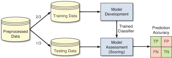
The main criticism of this method is that it makes the assumption that the data in the two subsets is of the same kind (i.e., has exactly the same properties). Because this is a simple random partitioning, in most realistic data sets where the data is skewed on the classification variable, such an assumption may not hold true. In order to improve this situation, stratified sampling is suggested, where the strata become the output variable. Even though this is an improvement over the simple split methodology, it still has a bias associated with the single random partitioning.
k-Fold Cross-Validation
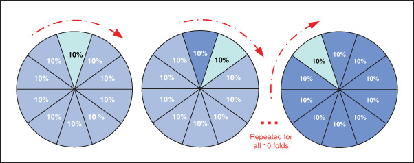
In order to minimize the bias associated with the random sampling of the training and holdout data samples in comparing the predictive accuracy of two or more methods, an analyst can use a methodology called k-fold cross-validation. In this methodology, also called rotation estimation, the complete data set is randomly split into k mutually exclusive subsets of approximately equal size. The classification model is trained and tested k times. Each time, it is trained on all but one fold and then tested on the remaining single fold. The cross-validation estimate of the overall accuracy of a model is calculated by simply averaging the k individual accuracy measures. This is the formula for this aggregation:
A graphical illustration of k-fold cross-validation, where the k is set to 10 (i.e., 10-fold cross-validation) is shown in Figure 4.6.
Other Classification Assessment Methodologies
Although not as common as the ones describe above, there are other assessment techniques used for classification type problems. Here are some of the most popular ones:
• Leave-one-out. The leave-one-out method is similar to a k-fold cross-validation where k takes the value 1; that is, every data point is used for testing once on as many models developed as there are data points. This is a time-consuming methodology, but it can be a viable option for small data sets.
• Bootstrapping. With bootstrapping, a fixed number of instances from the original data is sampled (with replacement) for training, and the rest of the data set is used for testing. This process is repeated as many times as desired.
• Jackknifing. This methodology is similar to the leave-one-out methodology; with it, accuracy is calculated by leaving one sample out at each iteration of the estimation process.
• Area under the ROC curve. The area under the ROC curve is a graphical assessment technique in which the true positive rate is plotted on the y-axis, and the false positive rate is plotted on the x-axis. The area under the ROC curve determines the accuracy measure of a classifier: A value of 1 indicates a perfect classifier, whereas 0.5 indicates no better than random chance, though in reality, the values would range between the two extreme cases. For example, in Figure 4.7, A has a better classification performance than B, while C is not any better than the random chance involved in flipping a coin.

Classification Methods
Many methods and algorithms are used for classification modeling, including the following:
• Decision tree analysis. Decision tree analysis (a machine learning technique) is arguably the most popular classification technique in the data mining arena. A detailed description of this technique is given in the following section.
• Statistical analysis. Statistical techniques were the primary classification algorithm for many years, until the emergence of machine learning techniques. Statistical classification techniques include logistic regression and discriminant analysis, both of which make the assumptions that the relationships between the input and output variables are linear in nature, the data is normally distributed, and the variables are not correlated and are independent of each other. The questionable nature of these assumptions has led to the shift toward machine learning techniques.
• Neural networks. Using neural networks is among the most popular machine learning techniques that can be used for classification-type problems. A detailed description of this technique is presented in Chapter 5.
• Support vector machines. Along with neural networks, support vector machines are also increasing in popularity as powerful classification algorithms. A detailed description of this technique is presented in Chapter 5.
• Nearest-neighbor algorithm. This deceptively simple yet highly efficient algorithm uses similarity as the basis for its classification method. A detailed description of this technique is also presented in Chapter 5.
• Case-based reasoning. Conceptually similar to the nearest-neighbor algorithm, this approach uses historical cases to recognize commonalities in order to assign a new case to the most probable category.
• Bayesian classifiers. This approach uses probability theory to build classification models based on the past occurrences that are capable of placing a new instance into a most probable class (or category).
• Genetic algorithms. Genetic algorithms use the analogy of natural evolution to build directed-search-based mechanisms to classify data samples.
• Rough sets. This method takes into account the partial membership of class labels to predefined categories in building models (collection of rules) for classification problems.
Complete coverage of all these classification techniques is beyond the scope of this book, so here we describe the most popular one, decision trees, and we cover a few of the other ones in Chapter 5.
Decision Trees
Before describing the details of decision trees, we need to discuss some simple terminology. First, decision trees include many input variables that may have an impact on the classification of different patterns. These input variables are usually called attributes. For example, if we were to build a model to classify loan risks on the basis of just two characteristics—income and credit rating—these two characteristics would be the attributes, and the resulting output would be the class label (e.g., low, medium, or high risk). Second, a tree consists of branches and nodes. A branch represents the outcome of a test to classify a pattern (on the basis of a test), using one of the attributes. A leaf node at the end represents the final class choice for a pattern (a chain of branches from the root node to the leaf node, which can be represented as a complex if–then statement).
The basic idea behind a decision tree is that it recursively divides a training set until each division consists entirely or primarily of examples from one class. Each nonleaf node of the tree contains a split point, which is a test on one or more attributes and determines how the data is to be divided further. Decision tree algorithms, in general, build an initial tree from the training data such that each leaf node is pure, and they then prune the tree to increase its generalization and, hence, the prediction accuracy of the test data.
In the growth phase, the tree is built by recursively dividing the data until each division is either pure (i.e., contains members of the same class) or relatively small. The basic idea is to ask questions whose answers provide the most information, as is done in the game “Twenty Questions.”
The split used to partition the data depends on the type of attribute used in the split. For a continuous attribute A, splits are of the form value(A) x, where x is some “optimal” split value of A. For example, the split based on income could be “Income > 50000.” For the categorical attribute A, splits are of the form value(A) belongs to x, where x is a subset of A. For example, the split could be on the basis of gender: male versus female.
A general algorithm for building a decision tree is as follows:
1. Create a root node and assign all the training data to it.
2. Select the best splitting attribute.
3. Add a branch to the root node for each value of the split. Split the data into mutually exclusive (i.e., non-overlapping) subsets along the lines of the specific split of the branches.
4. Repeat steps 2 and 3 for each leaf node until the stopping criteria is reached (e.g., the node is dominated by a single class label).
Many different algorithms have been proposed for creating decision trees. These algorithms differ primarily in terms of the way in which they determine the splitting attribute (and its split values), the order of splitting the attributes (splitting the same attribute only once or many times), the number of splits at each node (binary versus ternary), the stopping criteria, and the pruning of the tree (pre- versus postpruning). Some of the most well-known algorithms are ID3 (followed by C4.5 and C5 as the improved versions of ID3) from machine learning, classification and regression trees (CART) from statistics, and the chi-squared automatic interaction detector (CHAID) from pattern recognition.
When building a decision tree, the goal at each node is to determine the attribute and the split point of that attribute that best divides the training records in order to purify the class representation at that node. To evaluate the goodness of the split, some splitting indices have been proposed. Two of the most common ones are the Gini index and information gain. The Gini index is used in the CART and SPRINT (Scalable Parallelizable Induction of Decision Trees) algorithms. Versions of information gain are used in ID3 (and its newer versions, C4.5 and C5).
The Gini index has been used in economics to measure the diversity of a population. The same concept can be used to determine the purity of a specific class as a result of a decision to branch along a particular attribute or variable. The best split is the one that increases the purity of the sets resulting from a proposed split.
Information gain is the splitting mechanism used in ID3, which is perhaps the most widely known decision tree algorithm. It was developed by Ross Quinlan in 1986, and since then Quinlan has evolved this algorithm into the C4.5 and C5 algorithms. The basic idea behind ID3 and its variants is to use a concept called entropy in place of the Gini index. Entropy measures the extent of uncertainty or randomness in a data set. If all the data in a subset belongs to just one class, there is no uncertainty or randomness in that data set, so the entropy is zero. The objective of this approach is to build subtrees so that the entropy of each final subset is zero or close to zero.
Cluster Analysis for Data Mining
Cluster analysis is an essential data mining method for classifying items, events, or concepts into common groupings called clusters. The method is commonly used in biology, medicine, genetics, social network analysis, anthropology, archaeology, astronomy, character recognition, and even MIS development. As the popularity of data mining has increased, the underlying techniques have been applied to business, especially to marketing. Cluster analysis has been used extensively for fraud detection (both credit card and ecommerce fraud) and market segmentation of customers in contemporary CRM systems. More applications in business continue to be developed as the strength of cluster analysis is recognized and used.
Cluster analysis is an exploratory data analysis tool for solving classification problems. The objective is to sort cases (e.g., people, things, events) into groups, or clusters, so that the degree of association is strong among members of the same cluster and weak among members of different clusters. Each cluster describes the class to which its members belong. An obvious one-dimensional example of cluster analysis is to establish score ranges into which to assign class grades for a college class. This is similar to the cluster analysis problem that the U.S. Treasury faced when establishing new tax brackets in the 1980s. A fictional example of clustering occurs in J. K. Rowling’s Harry Potter books. The Sorting Hat determines to which House (e.g., dormitory) to assign first-year students at the Hogwarts School. Another example involves determining how to seat guests at a wedding. As far as data mining goes, the importance of cluster analysis is that it may reveal associations and structures in data that were not previously apparent but are sensible and useful once found.
Cluster analysis results may be used to:
• Identify a classification scheme (e.g., types of customers)
• Suggest statistical models to describe populations
• Indicate rules for assigning new cases to classes for identification, targeting, and diagnostic purposes
• Provide measures of definition, size, and change in what were previously broad concepts
• Find typical cases to label and represent classes
• Decrease the size and complexity of the problem space for other data mining methods
• Identify outliers in a specific domain (e.g., rare-event detection)
How to Determine the Number of Clusters
Clustering algorithms usually require specifying the number of clusters to find. If this number is not known from prior knowledge, it should be chosen in some way. Unfortunately, there is not an optimal way of calculating what this number is supposed to be. Therefore, several different heuristic methods have been proposed. The following are among the most commonly referenced ones:
• Look at the percentage of variance, expressed as a function of the number of clusters; that is, choose a number of clusters so that adding another cluster would not give much better modeling of the data. Specifically, in graphing the percentage of variance explained by the clusters, there is a point at which the marginal gain will drop (giving an angle in the graph), and this indicates the number of clusters to be chosen.
• Set the number of clusters to (n/2)1/2, where n is the number of data points.
• Use the Akaike information criterion (AIC), which is a measure of the goodness of fit (based on the concept of entropy) to determine the number of clusters.
• Use the Bayesian information criterion (BIC), which is a model-selection criterion (based on maximum likelihood estimation) to determine the number of clusters.
Clustering Methods
Cluster analysis involves grouping a set of records (samples, objects) in such a way that objects in the same group (called a cluster) are more similar to each other than to those in other groups (or clusters). Most cluster analysis methods involve the use of a distance measure to calculate the closeness between pairs of items. Popular distance measures include Euclidian distance (the ordinary distance between two points that one would measure with a ruler) and Manhattan distance (also called rectilinear distance, or taxicab distance, between two points). There are a number of cluster analysis techniques, each having a slightly different way of identifying natural grouping of objects or records. Figure 4.8 shows a simple taxonomy of clustering techniques.

As shown in Figure 4.8, at the highest level, the clustering methods can be classified as hierarchical and partitive. Hierarchical clustering methods are based on the basic idea that nearby objects are more related to each other than are those that are farther away. Therefore, a cluster can be defined by the maximum distance needed to connect all related objects. At different distances, different clusters would form, which can be represented using a dendrogram, which explains where the name hierarchical clustering comes from. In hierarchical clustering, the clusters can be identified either bottom-up (i.e., agglomerative—starting from the bottom, where each object is a cluster of its own and then adding similar objects to create more general clusters) or top-down (i.e., divisive—starting from the top cluster and then splitting the objects into more specific clusters).
Partitive clustering methods, on the other hand, are based on the idea that there are natural groups of objects in a multidimensional space. These methods follow the process of starting from an arbitrary number of clusters, assigning objects to most probable clusters, and then updating the number of clusters and evolving the assignment of objects to clusters until a stable cluster space is reached. The specific algorithms under partitive clustering use different ways to identify the clusters. Since there is not a single best method or algorithm for clustering, an analyst working with a clustering task should try several competing algorithms and assess their goodness of fit and identify the best one.
Assessment of a Clustering Technique
How do we measure the goodness of clusters created by a clustering method? How do we know if they are valid? How do we know to what extent they represent the natural grouping of the data? We need measures to compare how well different clustering algorithms perform on a given set of data. We can then choose the “best” one to use for a classification-type data mining problem. The measures for assessing the goodness of clustering methods are often grouped into two categories: internal assessment and external assessment.
Internal Assessment
Internal assessment methods usually assign the best assessment score to the method (or algorithm) that produces clusters with high similarity within a cluster and low similarity between clusters. The internal evaluation measures are best suited to situations where one algorithm performs better than another, but this may not imply that one algorithm produces more “valid” results than another. Validity is different from comparative assessment because it suggests that the identified cluster structure truly exists in the data set. This assessment methods measures intraclass and interclass similarities using some type of a distance measure in a multidimensional feature space.
One drawback of using internal criteria in cluster evaluation is that high scores on an internal measure do not necessarily result in effective information-retrieval applications. In addition, this evaluation is biased toward algorithms that use the same cluster model. For example, k-means clustering naturally optimizes object distances, and a distance-based internal criterion will likely overrate the resulting clustering.
External Assessment
Whereas in internal evaluation, clustering results are evaluated based on similarity measures, in external evaluation, the cluster results are measured based on data (with known class labels) that was not used for clustering. This assessment consists of a set of preclassified records, with known classes or class labels created by domain experts. Thus, the comparison sets can be thought of as a gold standard for evaluation. These types of evaluation methods measure how close the clustering is to the predetermined labeled classes. As logical as it may sound, widespread practicality of this method is questionable. Finding prelabeled classes for real-world data sets is difficult and may even be impossible. Also, because the true classes contain some type of natural structure, the attributes/variables presented to the clustering algorithm may not be complete enough to allow separation of true clusters.
k-Means Clustering Algorithm
The k-means algorithm (where k is the predetermined number of clusters) is arguably the most referenced clustering algorithm. It has its roots in traditional statistical analysis. As part of the family of centroid-based partitive clustering methods, the k-means algorithm, as its name implies, assigns each data point (e.g., customer, event, object) to the cluster whose center (also called centroid) is the nearest. The center is calculated as the average of all the points in the cluster; that is, its coordinates are the arithmetic mean for each dimension separately over all the points in the cluster. The algorithm steps are listed here and shown graphically in Figure 4.9:
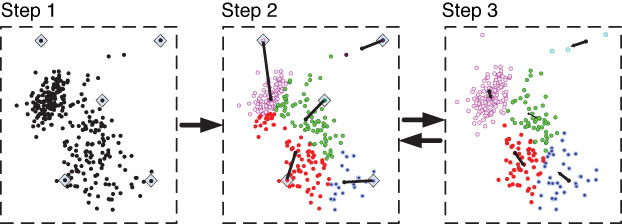
Initialization step: Choose the number of clusters (i.e., the value of k).
1. Randomly generate k random points as initial cluster centers.
2. Assign each point to the nearest cluster center.
3. Recompute the new cluster centers.
Repetition step: Repeat steps 2 and 3 until some convergence criterion is met (usually that the assignment of points to clusters becomes stable).
Association
Association—also known as association rule mining, or affinity analysis, or market-basket analysis—is a popular data mining method that is commonly used as an example to explain what data mining is and what it can do. You might have heard the famous (or infamous, depending on how you look at it) relationship discovered between the sales of beer and diapers at grocery stores. As the story goes, a large supermarket chain (maybe Wal-Mart, maybe not; there is no consensus on which supermarket chain it was) did an analysis of customers’ buying habits and found a statistically significant correlation between purchases of beer and purchases of diapers. It was theorized that the reason for this was that fathers (presumably young men) were stopping off at the supermarket to buy diapers for their babies (especially on Thursdays), and since they could no longer go down to the sports bar as often, they would buy beer as well. As a result of this finding, the supermarket chain is alleged to have placed the diapers next to the beer, resulting in increased sales of both.
In essence, association rule mining aims to find interesting relationships (affinities) between variables (items) in large databases. Because of its successful application to retail business problems, it is commonly called market-basket analysis. The main idea in market-basket analysis is to identify strong relationships among different products (or services) that are usually purchased together (i.e., show up in the same basket together, either a physical basket at a grocery store or a virtual basket at an ecommerce Website). For example, 65% of those who buy comprehensive automobile insurance also buy health insurance; 80% of those who buy books online also buy music online; 60% of those who have high blood pressure and are overweight have high cholesterol; 70% of the customers who buy laptop computer and virus protection software also buy extended service plans.
The input to market-basket analysis is simple point-of-sale transaction data, where a number of products and/or services purchased together (just like the content of a purchase receipt) are tabulated under a single transaction instance. The outcome of the analysis is invaluable information that can be used to better understand customer-purchase behavior in order to maximize the profit from business transactions. A business can take advantage of such knowledge by (1) putting the items next to each other to make it more convenient for the customers to pick them up together and not forget to buy one when buying the others (increasing sales volume); (2) promoting the items as a package (e.g., not putting one on sale if the other is on sale); and (3) placing the items apart from each other so that the customer has to walk the aisles to search for them and by doing so will potentially see and buy other items.
Applications of market-basket analysis include cross-marketing, cross-selling, store design, catalog design, ecommerce site design, optimization of online advertising, product pricing, and sales/promotion configuration. In essence, market-basket analysis helps businesses infer customer needs and preferences from their purchase patterns. Outside the business realm, association rules are successfully used to discover relationships between symptoms and illnesses, diagnosis and patient characteristics and treatments (which can be used in medical decision support systems [DSSs]), and genes and their functions (which can be used in genomics projects), among others. Here are a few common areas and uses for association rule mining:
• Sales transactions. Having knowledge of combinations of retail products purchased together can be used to improve product placement on sales floor (placing products that go together in close proximity) and promotional pricing of products (not having promotions on two products that are often purchased together).
• Credit card transactions. Having knowledge of items purchased with a credit card provides insight into other products the customer is likely to purchase or fraudulent use of a credit card number.
• Banking services. The sequential patterns of services used by customers (e.g., checking account followed by saving account) can be used to identify other services they may be interested in (e.g., investment account).
• Insurance service products. Bundles of insurance products bought by customers (e.g., car insurance followed by a home insurance) can be used to propose additional insurance products (e.g., life insurance); on the other hand, unusual combinations of insurance claims can be a sign of fraud.
• Telecommunication services. Commonly purchased group of options (e.g., call waiting, caller ID, three-way calling) help better structure product bundles to maximize revenue; this is also applicable to multichannel telecom providers with phone, television, and Internet service offerings.
• Medical records. Certain combinations of conditions can indicate increased risk of various complications; or certain treatment procedures at certain medical facilities can be tied to certain types of infection.
A good question to ask with respect to the patterns/relationships that association rule mining can discover is “Are all association rules interesting and useful?” In order to answer such a question, association rule mining uses three common metrics: support, confidence, and lift. Before defining these terms, let us look at what an association rule looks like. For example, in this rule, X (products and/or service; called the left-hand side [LHS], or antecedent) is associated with Y (products and/or service; called the right-hand side [RHS], or consequent):
X ⇒ Y [S(%), C(%)]
S is the support, and C is the confidence for this particular rule. Here are the simple formulas for support, confidence, and lift:

The support (S) of a collection of products and/or services is the measure of how often those products and/or services (i.e., LHS + RHS = laptop computer, antivirus software, and extended service plan) appear together in the same transaction—that is, the proportion of transactions in the data set that contain all the products and/or services mentioned in a specific rule. In this example, 30% of all transactions in the hypothetical store database had all three products present on a single sales ticket. The confidence of a rule is the measure of how often the products and/or services on the RHS (consequent) go together with the products and/or services on the LHS (antecedent)—that is, the proportion of transactions that include LHS while also including the RHS. In other words, it is the conditional probability of finding the RHS of the rule present in transactions where the LHS of the rule already exists. The lift value of an association rule is the ratio of the confidence of the rule and the expected confidence of the rule. The expected confidence of a rule is defined as the product of the support values of the LHS and the RHS divided by the support of the LHS.
Several algorithms are available for discovering association rules. Some well-known algorithms include Apriori, Eclat, and FP-Growth. These algorithms do only half the job, which is to identify the frequent item sets in the database. Once the frequent item sets are identified, they need to be converted into rules with antecedent and consequent parts. Determination of the rules from frequent item sets is a straightforward matching process, but the process may be time-consuming with large transaction databases. Even though there can be many items in each section of the rule, in practice the consequent part usually contains a single item. The following section explains one of the most popular algorithms for identification of frequent item sets.
Apriori Algorithm
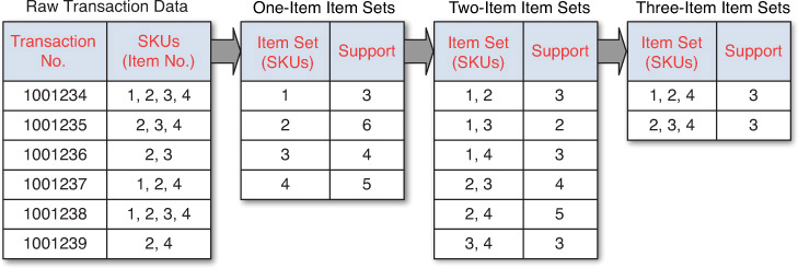
The Apriori algorithm is the algorithm most commonly used to discover association rules. Given a set of item sets (e.g., sets of retail transactions, each listing individual items purchased), the algorithm attempts to find subsets that are common to at least a minimum number of the item sets (i.e., comply with a minimum support). The Apriori algorithm uses a bottom-up approach, where frequent subsets are extended one item at a time (a method known as candidate generation, whereby the size of frequent subsets increases from one-item subsets to two-item subsets, then three-item subsets, etc.), and groups of candidates at each level are tested against the data for minimum support. The algorithm terminates when no further successful extensions are found.
As an illustrative example, consider the following. A grocery store tracks sales transactions by SKU (stock-keeping unit) and thus knows which items are typically purchased together. The database of transactions, along with the subsequent steps in identifying the frequent item sets, is shown in Figure 4.10. Each SKU in the transaction database corresponds to a product, such as “1 = butter,” “2 = bread,” “3 = water,” and so on. The first step in the Apriori algorithm is to count up the frequencies (i.e., the supports) of each item (one-item item sets). For this overly simplified example, let us set the minimum support to 3 (or 50%; meaning an item set is considered to be a frequent item set if it shows up in at least 3 out of 6 transactions in the database). Because all the one-item item sets have at least 3 in the support column, they are all considered frequent item sets. However, if any of the one-item item sets were not frequent, they would not have been included as possible members of possible two-item pairs. In this way, Apriori prunes the tree of all possible item sets. As Figure 4.10 shows, using one-item item sets, all possible two-item item sets are generated, and the transaction database is used to calculate their support values. Because the two-item item set {1, 3} has a support less than 3, it should not be included in the frequent item sets that will be used to generate the next-level item sets (three-item item sets). The algorithm seems deceptively simple, but only for small data sets. In much larger data sets, especially those with huge numbers of items present in low quantities and small numbers of items present in big quantities, the search and calculation become computationally intensive.
Data Mining Misconceptions and Realities
Data mining is a powerful analytical tool that enables business executives to advance from describing the nature of the past to predicting the future. It helps marketers find patterns that unlock the mysteries of customer behavior. The results of data mining can be used to increase revenue, reduce expenses, identify fraud, and locate business opportunities, offering a whole new realm of competitive advantage. As an evolving and maturing field, data mining is often associated with a number of misconceptions, including the ones listed in Table 4.3 (Zaima, 2003).

Data mining visionaries have gained enormous competitive advantage by understanding that these misconceptions are, in fact, misconceptions.
The following 10 data mining mistakes are often made in practice, and you should try to avoid them:
1. Selecting the wrong problem for data mining.
2. Ignoring what your sponsor thinks data mining is and what it really can and cannot do.
3. Leaving insufficient time for data preparation. This stage takes more effort than is generally understood.
4. Looking only at aggregated results and not at individual records. IBM’s DB2 IMS can highlight individual records of interest.
5. Being sloppy about keeping track of the data mining procedure and results.
6. Ignoring suspicious findings and quickly moving on.
7. Running mining algorithms repeatedly and blindly. It is important to think hard about the next stage of data analysis. Data mining is a very hands-on activity.
8. Believing everything you are told about the data.
9. Believing everything you are told about your own data mining analysis.
10. Measuring your results differently from the way your sponsor measures them.
Application Example: Predicting NCAA Bowl Game Results
Methodology
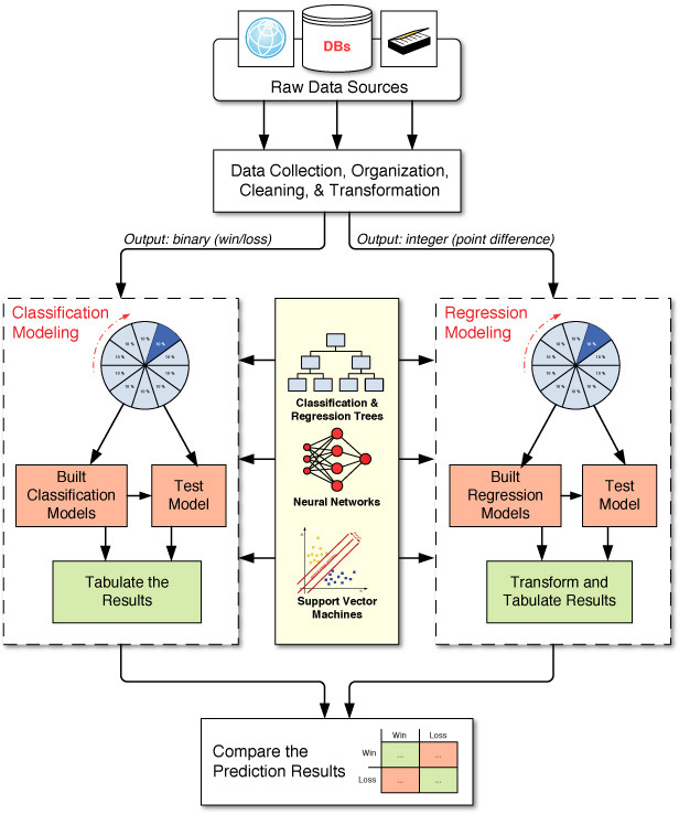
Data


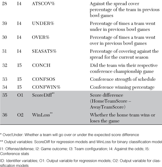
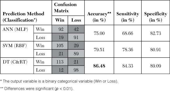
Evaluation
Results

Source: Delen, D., D. Cogdell, & N. Kasap, “A Comparative Analysis of Data Mining Methods in Predicting NCAA Bowl Outcomes,” International Journal of Forecasting, 28 (2012): 543–552.
References
Bhandari, I., et al. (1997). “Advanced Scout: Data Mining and Knowledge Discovery in NBA Data,” Data Mining and Knowledge Discovery, 1(1): 121–125.
Buck, N. (2000/2001, December/January). “Eureka! Knowledge Discovery,” Software Magazine.
Chan, P. K., W. Phan, A. Prodromidis, & S. Stolfo. (1999). “Distributed Data Mining in Credit Card Fraud Detection,” IEEE Intelligent Systems, 14(6): 67–74.
CRISP-DM. (2013). Cross-Industry Standard Process for Data Mining (CRISP-DM). www.the-modeling-agency.com/crisp-dm.pdf (accessed February 2013).
Davenport, T. H. (2006, January). “Competing on Analytics,” Harvard Business Review.
Delen, D., D. Cogdell, & N. Kasap. (2012). “A Comparative Analysis of Data Mining Methods in Predicting NCAA Bowl Outcomes,” International Journal of Forecasting, 28: 543–552.
Delen, D., R. Sharda, & P. Kumar. (2007). “Movie Forecast Guru: A Web-Based DSS for Hollywood Managers,” Decision Support Systems, 43(4): 1151–1170.
Nemati, H. R., & C. D. Barko. (2001). “Issues in Organizational Data Mining: A Survey of Current Practices,” Journal of Data Warehousing, 6(1): 25–36.
Quinlan, J. R. (1986). “Induction of Decision Trees,” Machine Learning, 1: 81–106.
Sharda, R., & D. Delen. (2006). “Predicting Box-Office Success of Motion Pictures with Neural Networks,” Expert Systems with Applications, 30: 243–254.
Stekler, H. O., D. Sendor, & R. Verlander. (2010). “Issues in Sports Forecasting,” International Journal of Forecasting, 26: 606–621.
Van Bruggen, G. H., M. Spann, G. L. Lilien, & B. Skiera. (2010). “Prediction Markets as Institutional Forecasting Support Systems,” Decision Support Systems, 49: 404–416.
Wald, M. L. (2004, February 21). “U.S. Calls Release of JetBlue Data Improper,” The New York Times.
Wilson, R., & R. Sharda. (1994). “Bankruptcy Prediction Using Neural Networks,” Decision Support Systems, 11: 545–557.
Wright, C. (2012). Statistical Predictors of March Madness: An Examination of the NCAA Men’s’ Basketball Championship. http://economics-files.pomona.edu/GarySmith/Econ190/Wright%20March%20Madness%20Final%20Paper.pdf (accessed February 2013).
Zaima, A. (2003). “The Five Myths of Data Mining,” What Works: Best Practices in Business Intelligence and Data Warehousing, 15: 42–43.