Chapter Four. Algorithms and Data Structures
This chapter presents fundamental data types that are essential building blocks for a broad variety of applications. We present full implementations, even though some of them are built into Python, so that you can have a clear idea of how they work and why they are important.
Objects can contain references to other objects, so we can build structures known as linked structures, which can be arbitrarily complex. With linked structures and arrays, we can build data structures to organize information in such a way that we can efficiently process it with associated algorithms. In a data type, we use the set of values to build data structures and the methods that operate on those values to implement algorithms.
The algorithms and data structures that we consider in this chapter introduce a body of knowledge developed over the past several decades that constitutes the basis for the efficient use of computers for a broad variety of applications. From n-body simulation problems in physics to genetic sequencing problems in bioinformatics, the basic approaches we describe have become essential in scientific research; from database systems to search engines, these methods are the foundation of commercial computing. As the scope of computing applications continues to expand, so grows the impact of these basic approaches.
Algorithms and data structures themselves are valid subjects of scientific inquiry. Accordingly, we begin by describing a scientific approach for analyzing the performance of algorithms, which we use throughout the chapter to study the performance characteristics of our implementations.
4.1 Performance
In this section, you will learn to respect a principle that is succinctly expressed in yet another mantra that should live with you whenever you program: Pay attention to the cost. If you become an engineer, that will be your job; if you become a biologist or a physicist, the cost will dictate which scientific problems you can address; if you are in business or become an economist, this principle needs no defense; and if you become a software developer, the cost will dictate whether the software that you build will be useful to your clients.
To study the cost of running them, we study our programs themselves via the scientific method, the commonly accepted body of techniques universally used by scientists to develop knowledge about the natural world. We also apply mathematical analysis to derive concise models of the cost.
Which features of the natural world are we studying? In most situations, we are interested in one fundamental characteristic: time. Whenever we run a program, we are performing an experiment involving the natural world, putting a complex system of electronic circuitry through series of state changes involving a huge number of discrete events that we are confident will eventually stabilize to a state with results that we want to interpret. Although developed in the abstract world of Python programming, these events most definitely are happening in the natural world. What will be the elapsed time until we see the result? It makes a great deal of difference to us whether that time is a millisecond, a second, a day, or a week. Therefore, we want to learn, through the scientific method, how to properly control the situation, just as when we launch a rocket, build a bridge, or smash an atom.
On the one hand, modern programs and programming environments are complex; on the other hand, they are developed from a simple (but powerful) set of abstractions. It is a small miracle that a program produces the same result each time we run it. To predict the time required, we take advantage of the relative simplicity of the supporting infrastructure that we use to build programs. You may be surprised at the ease with which you can develop cost estimates and predict the performance characteristics of many of the programs that you compose.
• Observe some feature of the natural world.
• Hypothesize a model that is consistent with the observations.
• Predict events using the hypothesis.
• Verify the predictions by making further observations.
• Validate by repeating until the hypothesis and observations agree.
One of the key tenets of the scientific method is that the experiments we design must be reproducible, so that others can convince themselves of the validity of the hypothesis. In addition, the hypotheses we formulate must be falsifiable—we have the possibility of knowing for sure when a hypothesis is wrong (and thus needs revision).
Observations
Our first challenge is to make quantitative measurements of the running time of our programs. Although measuring the exact running time of our program is difficult, usually we are happy with estimates. There are a number of tools available to help us obtain such approximations. Perhaps the simplest is a physical stopwatch or the Stopwatch data type (see PROGRAM 3.2.2). We can simply run a program on various inputs, measuring the amount of time to process each input.

Our first qualitative observation about most programs is that there is a problem size that characterizes the difficulty of the computational task. Normally, the problem size is either the size of the input or the value of a command-line argument. Intuitively, the running time should increase with the problem size, but the question of how much it increases naturally arises every time we develop and run a program.
Another qualitative observation for many programs is that the running time is relatively insensitive to the input itself; it depends primarily on the problem size. If this relationship does not hold, we need to run more experiments to better understand, and perhaps better control, the running time’s sensitivity to the input. Since this relationship does often hold, we focus now on the goal of better quantifying the correspondence between problem size and running time.
As a concrete example, we start with threesum.py (PROGRAM 4.1.1), which counts the number of triples in an array of n numbers that sum to 0. This computation may seem contrived to you, but it is deeply related to numerous fundamental computational tasks, particularly those found in computational geometry, so it is a problem worthy of careful study. What is the relationship between the problem size n and the running time for threesum.py?
Hypotheses
In the early days of computer science, Donald Knuth showed that, despite all of the complicating factors in understanding the running times of our programs, it is possible in principle to create accurate models that can help us predict precisely how long a particular program will take. Proper analysis of this sort involves:
• Detailed understanding of the program
• Detailed understanding of the system and the computer
• Advanced tools of mathematical analysis
Thus it is best left for experts. Every programmer, however, needs to know how to make back-of-the-envelope performance estimates. Fortunately, we can often acquire such knowledge by using a combination of empirical observations and a small set of mathematical tools.
Doubling hypotheses
For a great many programs, we can quickly formulate a hypothesis for the following question: What is the effect on the running time of doubling the size of the input? For clarity, we refer to this hypothesis as a doubling hypothesis. Perhaps the easiest way to pay attention to the cost is to ask yourself this question about your programs during development and also as you use them in practical applications. Next, we describe how to develop answers via the scientific method.
Empirical analysis
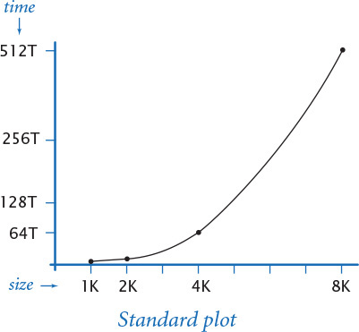
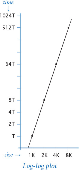
Clearly, we can get a headstart on developing a doubling hypothesis by doubling the size of the input and observing the effect on the running time. For example, doublingtest.py (PROGRAM 4.1.2) generates a sequence of random input arrays for threesum.py, doubling the array length at each step, and writes the ratio of running times of threesum.countTriples() for each input over the previous (which was one-half the size). If you run this program, you will find yourself caught in a prediction–verification cycle: It writes several lines very quickly, but then begins to slow down. Each time it writes a line, you find yourself wondering how long it will be until it writes the next line. Checking the stopwatch as the program runs, it is easy to predict that the elapsed time increases by about a factor of 8 to write each line. This prediction is verified by the Stopwatch measurements that the program writes, and leads immediately to the hypothesis that the running time increases by a factor of 8 when the input size doubles. We might also plot the running times, either on a standard plot (left), which shows that the rate of increase of the running time increases with input size, or on a log-log plot. In the case of threesum.py, the log-log plot (below) is a straight line with slope 3, which clearly suggests the hypothesis that the running time satisfies a power law of the form cn3 (see EXERCISE 4.1.29).
Program 4.1.1 3-sum problem (threesum.py)
import stdarray
import stdio
def writeTriples(a):
# See Exercise 4.1.1.
def countTriples(a):
n = len(a)
count = 0
for i in range(n):
for j in range(i+1, n):
for k in range(j+1, n):
if (a[i] + a[j] + a[k]) == 0:
count += 1
return count
def main():
a = stdarray.readInt1D()
count = countTriples(a)
stdio.writeln(count)
if count < 10:
writeTriples(a)
if __name__ == '__main__': main()
a[] | array of integers
n | length of a[]
count | number of triples that sum to 0
This program reads an array of integers from standard input, and writes to standard output the number of triples in the array that sum to 0. If the number is low, then it also writes the triples. The file 1000ints.txt contains 1,000 random 32-bit integers (between –231 and 231 – 1). Such a file is not likely to have such a triple (see EXERCISE 4.1.27).
% more 8ints.txt
8
30
-30
-20
-10
40
0
10
5
% python threesum.py < 8ints.txt
4
30 -30 0
30 -20 -10
-30 -10 40
-10 0 10
% python threesum.py < 1000ints.txt
0
Mathematical analysis
Knuth’s basic insight on building a mathematical model to describe the running time of a program is simple: the total running time is determined by two primary factors:
• The cost of executing each statement
• The frequency of execution of each statement
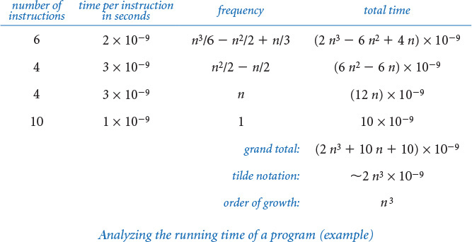
The former is a property of the system, and the latter is a property of the algorithm. If we know both for all instructions in the program, we can multiply them together and sum for all instructions in the program to get the running time.
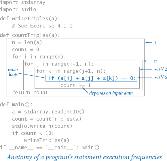
The primary challenge is to determine the frequency of execution of the statements. Some statements are easy to analyze; for example, the statement that initializes count to 0 in threesum.countTriples() is executed only once. Others require higher-level reasoning; for example, the if statement in threesum.countTriples() is executed precisely n (n–1)(n–2)/6 times (that is precisely the number of ways to pick three different numbers from the input array—see EXERCISE 4.1.5).
Frequency analyses of this sort can lead to complicated and lengthy mathematical expressions. To substantially simplify matters in the mathematical analysis, we develop simpler approximate expressions in two ways. First, we work with the leading term of mathematical expressions by using a mathematical device known as the tilde notation. We write ~ f(n) to represent any quantity that, when divided by f(n), approaches 1 as n grows. We also write g(n) ~ f(n) to indicate that g(n) / f(n) approaches 1 as n grows. With this notation, we can ignore complicated parts of an expression that represent small values. For example, the if statement in threesum.py is executed ~n3/6 times because n (n–1) (n–2) / 6 = n3/6 – n2/2 + n/3, which, when divided by n3/6, approaches 1 as n grows. This notation is useful when the terms after the leading term are relatively insignificant (for example, when n = 1,000, this assumption amounts to saying that –n2/2 + n/3 ≈ – 499,667 is relatively insignificant by comparison with n3/6 ≈ 166,666,667, which it is). Second, we focus on the instructions that are executed most frequently, sometimes referred to as the inner loop of the program. In this program it is reasonable to assume that the time devoted to the instructions outside the inner loop is relatively insignificant.
Program 4.1.2 Validating a doubling hypothesis (doublingtest.py)
import sys
import stdarray
import stdio
import stdrandom
import threesum
from stopwatch import Stopwatch
# Time to solve a random three-sum instance of size n.
def timeTrial(n):
a = stdarray.create1D(n, 0)
for i in range(n):
a[i] = stdrandom.uniformInt(-1000000, 1000000)
watch = Stopwatch()
count = threesum.countTriples(a)
return watch.elapsedTime()
n = int(sys.argv[1])
while True:
previous = timeTrial(n // 2)
current = timeTrial(n)
ratio = current / previous
stdio.writef('%7d %4.2f
', n, ratio)
n *= 2
n | problem size
a[] | random integers
watch | stopwatch
n | problem size
previous | running time for n // 2
current | running time for n
ratio | ratio of running times
This program writes to standard output a table of doubling ratios for the three-sum problem. The table shows how doubling the problem size affects the running time of the function call threesum.countTriples() for problem sizes that double for each row of the table. These experiments lead to the hypothesis that the running time increases by a factor of 8 when the input size doubles. When you run the program, note carefully that the elapsed time increases by a factor of 8 for each line written, validating the hypothesis.
% python doublingtest.py 256
256 7.52
512 8.09
1024 8.07
2048 7.97
...
The key point in analyzing the running time of a program is this: for a great many programs, the running time satisfies the relationship
T(n) ∼ c f(n)

where c is a constant and f(n) is a function known as the order of growth of the running time. For typical programs, f(n) is a function such as log n, n, n log n, n2, or n3, as you will soon see (customarily, we express order-of-growth functions without any constant coefficient). When f(n) is a power of n, as is often the case, this assumption is equivalent to saying that the running time satisfies a power law. In the case of threesum.py, it is a hypothesis already verified by our empirical observations: the order of growth of the running time of threesum.py is n3. The value of the constant c depends both on the cost of executing instructions and on details of the frequency analysis, but we normally do not need to work out the value, as you will now see.
The order of growth is a simple but powerful model of running time. For example, knowing the order of growth typically leads immediately to a doubling hypothesis. In the case of threesum.py, knowing that the order of growth is n3 tells us to expect the running time to increase by a factor of 8 when we double the size of the problem because
T(2n)/T(n) → c (2n)3/(cn3) = 8
This matches the value resulting from the empirical analysis, thus validating both the model and the experiments. Study this example carefully, because you can use the same method to better understand the performance of any program that you compose.
Knuth showed that it is possible to develop an accurate mathematical model of the running time of any program, and many experts have devoted much effort to developing such models. But you do not need such a detailed model to understand the performance of your programs: it is typically safe to ignore the cost of the instructions outside the inner loop (because that cost is negligible by comparison to the cost of the instruction in the inner loop) and not necessary to know the value of the constant in the running-time approximation (because it cancels out when you use a doubling hypothesis to make predictions).
These approximations are significant because they relate the abstract world of a Python program to the real world of a computer running it. The approximations are such that characteristics of the particular machine that you are using do not play a significant role in the models—the analysis separates the algorithm from the system. The order of growth of the running time of threesum.py is n3 does not depend on whether it is implemented in Python or whether it is running on your laptop, someone else’s mobile phone, or a supercomputer; rather, it depends primarily on the fact that it examines all the triples. The properties of the computer and the system are all summarized in various assumptions about the relationship between program statements and machine instructions, and in the actual running times that we observe as the basis for the doubling hypothesis. The algorithm that you are using determines the order of growth. This separation is a powerful concept because it allows us to develop knowledge about the performance of algorithms and then apply that knowledge to any computer. In fact, much of the knowledge about the performance of classic algorithms was developed decades ago, but that knowledge is still relevant to today’s computers.
Empirical and mathematical analyses like those we have described constitute a model (an explanation of what is going on) that might be formalized by listing all of the assumptions mentioned (each instruction takes the same amount of time each time it is executed, running time has the given form, and so forth). Not many programs are worthy of a detailed model, but you need to have an idea of the running time that you might expect for every program that you compose. Pay attention to the cost. Formulating a doubling hypothesis—through empirical studies, mathematical analysis, or (preferably) both—is a good way to start. This information about performance is extremely useful, and you will soon find yourself formulating and validating hypotheses every time you run a program. Indeed, doing so is a good use of your time while you wait for your program to finish!
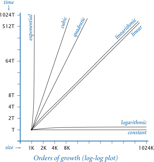
Order of growth classifications
We use just a few structural primitives (statements, conditionals, loops, and function calls) to build Python programs, so very often the order of growth of our programs is one of just a few functions of the problem size, summarized in the table on the next page. These functions immediately lead to a doubling hypothesis, which we can verify by running the programs. Indeed, you have been running programs that exhibit these orders of growth, as you can see in the following brief discussions.
Constant
A program whose running time’s order of growth is constant executes a fixed number of statements to finish its job; consequently, its running time does not depend on the problem size. Our first several programs in CHAPTER 1—such as helloworld.py (PROGRAM 1.1.1) and leapyear.py (PROGRAM 1.2.5)—fall into this category: they each execute several statements just once.

All of Python’s operations on standard numeric types take constant time. That is, applying an operation to a large number consumes no more time than does applying it to a small number. (One exception is that operations involving integers with a huge number of digits can consume more than constant time; see the Q&A at the end of this section for details.) The functions in Python’s math module also take constant time. Note that we do not specify the size of the constant. For example, the constant for math.atan2() is somewhat larger than the constant for math.hypot().
Logarithmic
A program whose running time’s order of growth is logarithmic is barely slower than a constant-time program. The classic example of a program whose running time is logarithmic in the problem size is looking for an element in a sorted array, which we consider in the next section (see PROGRAM 4.2.3, binarysearch.py). The base of the logarithm is not relevant with respect to the order of growth (since all logarithms with a constant base are related by a constant factor), so we use log n when referring to the order of growth. Occasionally, we write more precise formulas using lg n (base 2, or binary log) or ln n (base e, or natural logarithm) because both arise naturally when studying computer programs. For example, lg n, rounded up, is the number of bits in the binary representation of n, and ln n arises in the analysis of binary search trees (see SECTION 4.4).
Linear
Programs that spend a constant amount of time processing each piece of input data, or that are based on a single for loop, are quite common. The order of growth of such a program is said to be linear—its running time is directly proportional to the problem size. PROGRAM 1.5.3 (average.py), which computes the average of the numbers on standard input, is prototypical, as is our code to shuffle the elements in an array in SECTION 1.4. Filters such as plotfilter.py (PROGRAM 1.5.5) also fall into this category, as do the various image-processing filters that we considered in SECTION 3.2, which perform a constant number of arithmetic operations per input pixel.
Linearithmic
We use the term linearithmic to describe programs whose running time for a problem of size n has order of growth n log n. Again, the base of the logarithm is not relevant. For example, couponcollector.py (PROGRAM 1.4.2) is linearithmic. The prototypical example is mergesort (see PROGRAM 4.2.6). Several important problems have natural solutions that are quadratic but clever algorithms that are linearithmic. Such algorithms (including mergesort) are critically important in practice because they enable us to address problem sizes far larger than could be addressed with quadratic solutions. In the next section, we consider a general design technique for developing linearithmic algorithms.
Quadratic
A typical program whose running time has order of growth n2 has two nested for loops, used for some calculation involving all pairs of n elements. The force update double loop in universe.py (PROGRAM 3.4.2) is a prototype of the programs in this classification, as is the elementary sorting algorithm insertion sort (see PROGRAM 4.2.4).
Cubic
Our example for this section, threesum.py, is cubic (its running time has order of growth n3) because it has three nested for loops, to process all triples of n elements. The running time of matrix multiplication, as implemented in SECTION 1.4 has order of growth m3 to multiply two m-by-m matrices, so the basic matrix multiplication algorithm is often considered to be cubic. However, the size of the input (the number of elements in the matrices) is proportional to n = m2, so the algorithm is best classified as n3/2, not cubic.


Exponential
As discussed in SECTION 2.3, both towersofhanoi.py (PROGRAM 2.3.2) and beckett.py (PROGRAM 2.3.3) have running times proportional to 2n because they process all subsets of n elements. Generally, we use the term “exponential” to refer to algorithms whose order of growth is bn for any constant b > 1, even though different values of b lead to vastly different running times. Exponential algorithms are extremely slow—you should never run one of them for a large problem. They play a critical role in the theory of algorithms because there exists a large class of problems for which it seems that an exponential algorithm is the best possible choice.
These classifications are the most common, but certainly not a complete set. Indeed, the detailed analysis of algorithms can require the full gamut of mathematical tools that have been developed over the centuries. Understanding the running time of programs such as factors.py (PROGRAM 1.3.9), primesieve.py (PROGRAM 1.4.3), and euclid.py (PROGRAM 2.3.1) requires fundamental results from number theory. Classic algorithms like hashst.py (PROGRAM 4.4.3) and bst.py (PROGRAM 4.4.4) require careful mathematical analysis. The programs sqrt.py (PROGRAM 1.3.6) and markov.py (PROGRAM 1.6.3) are prototypes for numerical computation: their running time depends on the rate of convergence of a computation to a desired numerical result. Monte Carlo simulations such as gambler.py (PROGRAM 1.3.8) and percolation.py (PROGRAM 2.4.6) and variants are of interest precisely because detailed mathematical models for them are not available.
Nevertheless, a great many of the programs that you will compose have straightforward performance characteristics that can be described accurately by one of the orders of growth that we have considered, as documented in the table on the preceding page. Accordingly, we can usually work with simple higher-level hypotheses, such as the order of growth of the running time of mergesort is linearithmic. For economy, we abbreviate such a statement to just say mergesort is linearithmic. Most of our hypotheses about cost are of this form, or of the form mergesort is faster than insertion sort. Again, a notable feature of such hypotheses is that they are statements about algorithms, not just about programs.
Predictions
You can always try to estimate the running time of a program by simply running it, but that might be a poor way to proceed when the problem size is large. In that case, it is analogous to trying to estimate where a rocket will land by launching it, how destructive a bomb will be by igniting it, or whether a bridge will stand by building it.
Knowing the order of growth of the running time allows us to make decisions about addressing large problems so that we can invest whatever resources we have to deal with the specific problems that we actually need to solve. We typically use the results of verified hypotheses about the order of growth of the running time of programs in one of the following ways.
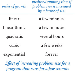
Estimating the feasibility of solving large problems
To pay attention to the cost, you need to answer this basic question for every program that you compose: Will this program be able to process this input data in a reasonable amount of time? For example, a cubic algorithm that runs in a couple of seconds for a problem of size n will require a few weeks for a problem of size 100n because it will be a million (1003) times slower, and a couple of million seconds is a few weeks. If that is the size of the problem that you need to solve, you have to find a better method. Knowing the order of growth of the running time of an algorithm provides precisely the information that you need to understand limitations on the size of the problems that you can solve. Developing such understanding is the most important reason to study performance. Without it, you are likely have no idea how much time a program will consume; with it, you can perform a back-of-the-envelope calculation to estimate costs and proceed accordingly.
Estimating the value of using a faster computer
To pay attention to the cost, you also may be faced with this basic question: How much faster can I solve a problem if I run it on a faster computer? Again, knowing the order of growth of the running time provides precisely the information that you need. A famous rule of thumb known as Moore’s law implies that you can expect to have a computer with about double the speed and double the memory 18 months from now, or a computer with about 10 times the speed and 10 times the memory in about 5 years. It is natural to think that if you buy a new computer that is 10 times faster and has 10 times more memory than your old one, you can solve a problem 10 times the size, but that is unmistakably not the case for quadratic or cubic algorithms. Whether it is an investment banker running daily financial models or a scientist running a program to analyze experimental data or an engineer running simulations to test a design, it is not unusual for people to regularly run programs that take several hours to complete. Suppose that you are using a program whose running time is cubic, and then buy a new computer that is 10 times faster with 10 times more memory, not just because you need a new computer, but because you face problem sizes that are 10 times larger. The rude awakening is that your program will take 100 times longer than before! This kind of situation is the primary reason that linear and linearithmic algorithms are so valuable: with such an algorithm and a new computer that is 10 times faster with 10 times more memory than the old computer, you can solve a problem that is 10 times larger than could be solved by the old computer in the same amount of time. In other words, you cannot keep pace with Moore’s law if you are using a quadratic or a cubic algorithm.

Comparing programs
We always seek ways to improve our programs, and we can often extend or modify our hypotheses to evaluate the effectiveness of various improvements. With the ability to predict performance, we can make design decisions during development that can guide us toward better, more efficient implementations. In many cases, we can determine the order of growth of the running times and develop accurate hypotheses about comparative performance. The order of growth is extremely useful in this process because it allows us to compare one particular algorithm with whole classes of algorithms. For example, once we have a linearithmic algorithm to solve a problem, we become less interested in quadratic or cubic algorithms to solve the same problem.
Caveats
There are many reasons that you might get inconsistent or misleading results when trying to analyze program performance in detail. All of them have to do with the idea that one or more of the basic assumptions underlying our hypotheses might not be quite correct. We can develop new hypotheses based on new assumptions, but the more details that we take into account, the more care we need in the analysis.
Instruction time
The assumption that each instruction always takes the same amount of time is not always correct. For example, most modern computer systems use a technique known as caching to organize memory, in which case accessing elements in huge arrays can take much longer if they are not close together in the array. You may be able to observe the effect of caching for threesum.py by letting doublingtest.py run for a while. After seeming to converge to 8, the ratio of running times may jump to a larger value for large arrays because of caching.
Nondominant inner loop
The assumption that the inner loop dominates may not always be correct. The problem size n might not be sufficiently large to make the leading term in the mathematical description of the frequency of execution of instructions in the inner loop so much larger than lower-order terms that we can ignore them. Some programs have a significant amount of code outside the inner loop that needs to be taken into consideration.
System considerations
Typically, there are many, many things going on in your computer. Python is just one application of many competing for resources, and Python itself has many options and controls that significantly affect performance. Such considerations can interfere with the bedrock principle of the scientific method that experiments should be reproducible, since what is happening at this moment in your computer will never be reproduced again. Whatever else is going on in your system (that is beyond your control) should in principle be negligible.
Too close to call
Often, when we compare two different programs for the same task, one might be faster in some situations, and slower in others. One or more of the considerations just mentioned could make the difference. Again, there is a natural tendency among some programmers (and some students) to devote an extreme amount of energy running such horseraces to find the “best” implementation, but such work is best left for experts.
Strong dependence on input values
One of the first assumptions that we made to determine the order of growth of the program’s running time of a program was that the running time should be relatively insensitive to the input values. When that is not the case, we may get inconsistent results or be unable to validate our hypotheses. Our running example threesum.py does not have this problem, but we will see several examples in this chapter of programs whose running time does depends on the input values. Often, a prime design goal is to eliminate such dependence on the input values. If we cannot do so, we need to more carefully model the kind of input to be processed in the problems that we need to solve, which may be a significant challenge. For example, if we are composing a program to process a genome, how do we know how it will perform on a different genome? But a good model describing the genomes found in nature is precisely what scientists seek, so estimating the running time of our programs on data found in nature actually makes a valuable contribution to that model!
Multiple problem parameters
We have been focusing on measuring performance as a function of a single parameter n, generally the value of a command-line argument or the size of the input. However, it is not unusual to measure performance using two (or more) parameters. For example, suppose that a[] is an array of length m and b[] is an array of length n. Consider the following code fragment that counts the number of pairs i and j for which a[i] + b[j] equals 0:
for i in range(m):
for j in range(n):
if a[i] + b[j] == 0:
count += 1
In such cases, we treat the parameters m and n separately, holding one fixed while analyzing the other. For example, the order of growth of the running time of this code fragment is mn.
Despite all these caveats, understanding the order of growth of the running time of each program is valuable knowledge for any programmer, and the methods that we have described are powerful and broadly applicable. Knuth’s insight was that we can carry these methods through to the last detail in principle to make detailed, accurate predictions. Typical computer systems are extremely complex and close analysis is best left for experts, but the same methods are effective for developing approximate estimates of the running time of any program. A rocket scientist needs to have some idea of whether a test flight will land in the ocean or in a city; a medical researcher needs to know whether a drug trial will kill or cure all the subjects; and any scientist or engineer using a computer program needs to have some idea of whether it will run for a second or for a year.
Performance guarantees
For some programs, we demand that the running time of a program is less than a certain bound for any input of a given size. To provide such performance guarantees, theoreticians take an extremely pessimistic view: what would the running time be in the worst case?
For example, such a conservative approach might be appropriate for the software that runs a nuclear reactor or an air traffic control system or the brakes in your car. We must guarantee that such software completes its job within the bounds that we set because the result could be catastrophic if it does not. Scientists normally do not contemplate the worst case when studying the natural world: in biology, the worst case might the extinction of the human race; in physics, the worst case might be the end of the universe. But the worst case can be a very real concern in computer systems, where the input is generated by another (potentially malicious) user, rather than by nature. For example, websites that do not use algorithms with performance guarantees are subject to denial-of-service attacks, where hackers flood them with pathological requests that make them run harmfully slower than planned.
Performance guarantees are difficult to verify with the scientific method, because we cannot test a hypothesis such as mergesort is guaranteed to be linearithmic without trying all possible inputs, which we cannot do because there are far too many of them. We might falsify such a hypothesis by providing inputs for which mergesort is slow, but how can we prove it to be true? We must do so not with experimentation, but rather with mathematical models.
It is the task of the algorithm analyst to discover as much relevant information about an algorithm as possible, and it is the task of the applications programmer to apply that knowledge to develop programs that effectively solve the problems at hand. For example, if you are using a quadratic algorithm to solve a problem but can find an algorithm that is guaranteed to be linearithmic, you will usually prefer the linearithmic one. On rare occasions, you might still prefer the quadratic algorithm because it is faster on the kinds of inputs that you need to solve or because the linearithmic algorithm is too complex to implement.
Ideally, we want algorithms that lead to clear and compact code that provides both a good worst-case guarantee and good performance on inputs of interest. Many of the classic algorithms that we consider in this chapter are of importance for a broad variety of applications precisely because they have all of these properties. Using these algorithms as models, you can develop good solutions yourself for typical problems that you face while programming.
Python lists and arrays
Python’s built-in list data type represents a mutable sequence of objects. We have been using Python lists throughout the book—recall that we use Python lists as arrays because they support the four core array operations: creation, indexed access, indexed assignment, and iteration. However, Python lists are more general than arrays because you can also insert items into and delete items from Python lists. Even though Python programmers typically do not distinguish between lists and arrays, many other programmers do make such a distinction. For example, in many programming languages, arrays are of fixed length and do not support insertions or deletions. Indeed, all of the array-processing code that we have considered in this book so far could have been done using fixed-length arrays.

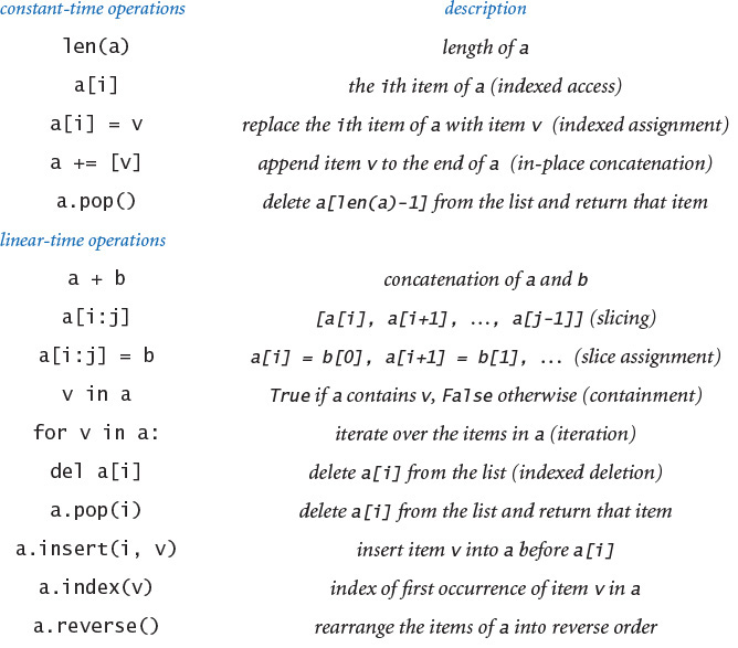
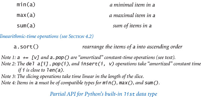
The table on the facing page gives the most commonly used operations for Python lists. Note that several of these operations—indexing, slicing, concatenation, deletion, containment, and iteration—enjoy direct language support in the form of special syntax. As illustrated in the table at right, some of these operations return values while others mutate the invoking list.
We have deferred this API to this section because programmers who use Python lists without following our mantra pay attention to the cost are in for trouble. For example, consider these two code snippets:
# quadratic time # linear time
a = [] a = []
for i in range(n): for i in range(n):
a .insert(0, 'slow') a.insert(i, 'fast')
The one on the left takes quadratic time; the one on the right takes linear time. To understand why Python list operations have the performance characteristics that they do, you need to learn more about Python’s resizing array representation of lists, which we discuss next.
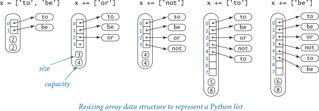
Resizing arrays
A resizing array is a data structure that stores a sequence of items (not necessarily fixed in length), which can be accessed by indexing. To implement a resizing array (at the machine level), Python uses a fixed-length array (allocated as one contiguous block of memory) to store the item references. The array is divided into two logical parts: the first part of the array contains the items in the sequence; the second part of the array is unused and reserved for subsequent insertions. Thus, we can append or remove items from the end in constant time, using the reserved space. We use the term size to refer to the number of items in the data structure and the term capacity to refer to the length of the underlying array.
The main challenge is ensuring that the data structure has sufficient capacity to hold all of the items, but is not so large as to waste an excessive amount of memory. Achieving these two goals turns out to be remarkably easy.
First, if we want to append an item to the end of a resizing array, we check its capacity. If there is room, we simply insert the new item at the end. If not, we double its capacity by creating a new array of twice the length and copying the items from the old array into the new array.
Similarly, if we want to remove an item from the end of the resizing array, we check its capacity. If it is excessively large, we halve its capacity by creating a new array of half the length and copying the items from the old array into the new array. An appropriate test is to check whether the size of the resizing array is less than one-fourth of its capacity. That way, after the capacity is halved, the resizing array is about half full and can accommodate a substantial number of insertions before we have to change its capacity again.
The doubling-and-halving strategy guarantees that the resizing array remains between 25% and 100% full, so that space is linear in the number of items. The specific strategy is not sacrosanct. For example, typical Python implementations expand the capacity by a factor of 9/8 (instead of 2) when the resizing array is full. This wastes less space (but triggers more expansion and shrinking operations).
Amortized analysis
The doubling-and-halving strategy is a judicious tradeoff between wasting space (by setting the capacity to be too large and leaving much of the array unused) and wasting time (either by creating a new array or by reorganizing the existing array). More important, we can prove that the cost of doubling and halving is always absorbed (to within a constant factor) in the cost of other Python list operations.
More precisely, starting from an empty Python list, any sequence of n operations labeled as “constant time” in the API table on page 531 takes time linear in n. In other words, the total cost of any such sequence of Python list operations divided by the number of operations is bounded by a constant. This kind of analysis is known as amortized analysis. This guarantee is not as strong as saying that each operation is constant-time, but it has the same implications in many applications (for example, when our primary interest is in total running time). We leave the full details as an exercise for the mathematically inclined.
For the special case where we perform a sequence of n insertions into an empty resizing array, the idea is simple: each insertion takes constant time to add the item; each insertion that triggers a resizing (when the current size is a power of 2) takes additional time proportional to n to copy the elements from the old array of length n to a new array of length 2n. Thus, assuming n is a power of 2 for simplicity, the total cost is proportional to
(1 + 1 + 1 + ... + 1) + (1 + 2 + 4 + 8 + ... + n) ~ 3n
The first term (which sums to n) accounts for the n insertion operations; the second term (which sums to 2n − 1) accounts for the lg n resizing operations.
Understanding resizing arrays is important in Python programming. For example, it explains why creating a Python list of n items by repeatedly appending items to the end takes time proportional to n (and why creating a list of n items by repeatedly prepending items to the front takes time proportional to n2). Such performance pitfalls are precisely the reason that we recommend using narrower interfaces that address performance.
Strings
Python’s string data type has some similarity to Python lists, with one very important exception: strings are immutable. When we introduced strings, we did not emphasize this fact, but it makes lists and strings quite different. For example, you may not have noticed at the time, but you cannot change a character in a string. For example, you might think that you could capitalize a string s having the value 'hello' with s[0] = 'H', but that will result in this run-time error:
TypeError: 'str' object does not support item assignment
If you want 'Hello', you need to create a completely new string. This difference reinforces the idea of immutability and has significant implications with regard to performance, which we now examine.
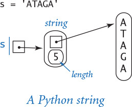
Internal representation
First, Python uses a much simpler internal representation for strings than for lists/arrays, as detailed in the diagram at left. Specifically, a string object contains two pieces of information:
• A reference to a place in memory where the characters in the string are stored contiguously
• The length of the string
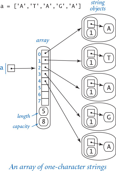
By contrast, consider the diagram at right, which is an array of one-character strings. We will consider a more detailed analysis later in this section, but you can see that the string representation is certainly significantly simpler. It uses much less space per character and provides faster access to each character. In many applications, these characteristics are very important because strings can be very long. So, it is important both that the memory usage be not much more than is required for the characters themselves and that characters can be quickly accessed by their index, as in an array.
Performance
As for arrays, indexed access and computing the length of strings are constant-time operations. It is clear from the API at the beginning of SECTION 3.1 that most other operations take linear time as a function of the length of the input string or strings, because they refer to a copy of the string. In particular, concatenating a character to a string takes linear time and concatenating two strings takes time proportional to the length of the result. An example is shown at right. With respect to performance, this is the most significant difference between strings and lists/arrays: Python does not have resizable strings, because strings are immutable.
Example
Not understanding the performance of string concatenation often leads to performance bugs. The most common performance bug is building up a long string one character at a time. For example, consider the following code fragment to create a new string whose characters are in reverse order of the characters in a string s:
n = len(s)
reverse = ''
for i in range(n):
reverse = s[i] + reverse
During iteration i of the for loop, the string concatenation operator produces a string of length i+1. Thus, the overall running time is proportional to 1 + 2 + ... + n ~ n2 / 2 (see EXERCISE 4.1.4). That is, the code fragment takes quadratic time as a function of the string length n (see EXERCISE 4.1.13 for a linear-time solution).

Understanding differences between data types like strings and Python lists is critical in learning any programming language, and programmers must be vigilant to ensure they avoid performance bugs like the one just described. This has been the case since the early days of data abstraction. For example, the string data type in the C language that was developed in the 1970s has a linear-time length function, and countless programmers using the length in a for loop that iterates through the string have found themselves with a quadratic-time performance bug for a simple linear-time job.
Memory
As with running time, a program’s memory usage connects directly to the physical world: a substantial amount of your computer’s circuitry enables your program to store values and later retrieve them. The more values you need to store at any given instant, the more circuitry you need. To pay attention to the cost, you need to be aware of memory usage. You probably are aware of limits on memory usage on your computer (even more so than for time) because you probably have paid extra money to get more memory.
At the outset, you should be aware that the flexibility that we get from Python’s pure approach to object-oriented programming (everything is an object, even boolean values) comes with costs, and one of the most significant costs is the amount of memory consumed. This will become more clear as we examine some specific examples.
Memory usage is well defined for Python on your computer (every value will require precisely the same amount of memory each time that you run your program), but Python is implemented on a very wide range of computational devices, and memory consumption is implementation-dependent. Different versions of Python might implement the same data type in different ways. For economy, we use the word typical to signal values that are particularly subject to machine dependencies. Analyzing memory usage is somewhat different from analyzing time usage, primarily because one of Python’s most significant features is its memory allocation system, which is supposed to relieve you of having to worry about memory. Certainly, you are well advised to take advantage of this feature when appropriate. Still, it is your responsibility to know, at least approximately, when a program’s memory requirements might prevent you from solving a given problem.
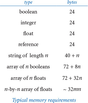
Computer memory is divided into bytes, where each byte consists of 8 bits, and where each bit is a single binary digit. To determine the memory usage of a Python program, we count up the number of objects used by the program and weight them by the number of bytes that they require, according to their type. To use that approach, we must know the number of bytes consumed by an object of any given type. To determine the memory consumption of an object, we add the amount of memory used by each of its instance variables to the overhead associated with each object.
Python does not define the sizes of the built-in data types that we have been using (int, float, bool, str, and list); the sizes of objects of those types differ from system to system. Accordingly, the sizes of data types that you create also will differ from system to system because they are based on these built-in data types. The function call sys.getsizeof(x) returns the number of bytes that a built-in object x consumes on your system. The numbers that we give in this section are observations gathered by using this function in interactive Python on one typical system. We encourage you to do the same on your computer!
Python 3 alert
The numbers we give in this section are for a typical Python 2 system. Python 3 uses a more complicated memory model. For example, the memory used by the int object 0 is not the same as the memory used by the int object 1.
Integers
To represent an int object whose value is in the range (–263 to 263 – 1), Python uses 16 bytes for overhead and 8 bytes (that is, 64 bits) for the numeric value. So, for example, Python uses 24 bytes to represent the int object whose value is 0, 24 bytes to represent the int object whose value is 1234, and so forth. In most applications, we are not dealing with huge integers outside this range, so the memory consumption for each integer is 24 bytes. Python switches to a different internal representation for integers outside this range, which consumes memory proportional to the number of digits in the integer, as in the case with strings (see below).
Floats
To represent a float object, Python uses 16 bytes for overhead and 8 bytes for the numeric value (that is, the mantissa, exponent, and sign), no matter what value the object has. So a float object always consumes 24 bytes.

Booleans
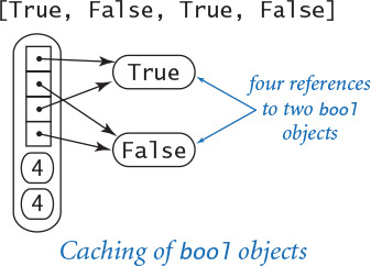
In principle, Python could represent a boolean value using a single bit of computer memory. In practice, Python represents boolean values as integers. Specifically, Python uses 24 bytes to represent the bool object True and 24 bytes to represent the bool object False. That is a factor of 192 higher than the minimum amount needed! However, this wastefulness is partially mitigated because Python “caches” the two boolean objects, as we discuss next.
Caching
To save memory, Python creates only one copy of objects with certain values. For example, Python creates only one bool object with value true and only one with value false. That is, every boolean variables holds a reference to one of these two objects. This caching technique is possible because the bool data type is immutable. On typical systems, Python also caches small int values (between –5 and 256), as they are the ones that programmers use most often. Python does not typically cache float objects.
Strings
To represent a str object, Python uses 40 bytes for overhead (including the string length), plus one byte for each character of the string. So, for example, Python represents the string 'abc' using 40 + 3 = 43 bytes and represents the string 'abcdefghijklmnopqr' using 40 + 18 = 58 bytes. Python typically caches only string literals and one-character strings.
Arrays (Python lists)
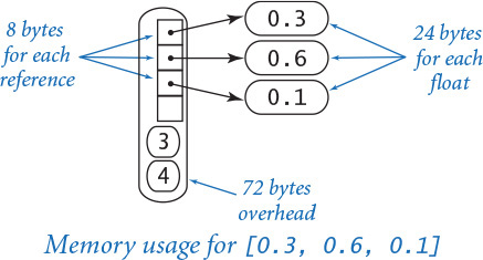
To represent an array, Python uses 72 bytes for overhead (including the array length) plus 8 bytes for each object reference (one for each element in the array). So, for example, the Python representation of the array [0.3, 0.6, 0.1] uses 72 + 8*3 = 96 bytes. This does not include the memory for the objects that the array references, so the total memory consumption for the array [0.3, 0.6, 0.1] is 96 + 3*24 = 168 bytes. In general, the memory consumption for an array of n integers or floats is 72 + 32n bytes. This total is likely to be an underestimate, because the resizing array data structure that Python uses to implement arrays may consume an additional n bytes in reserved space.
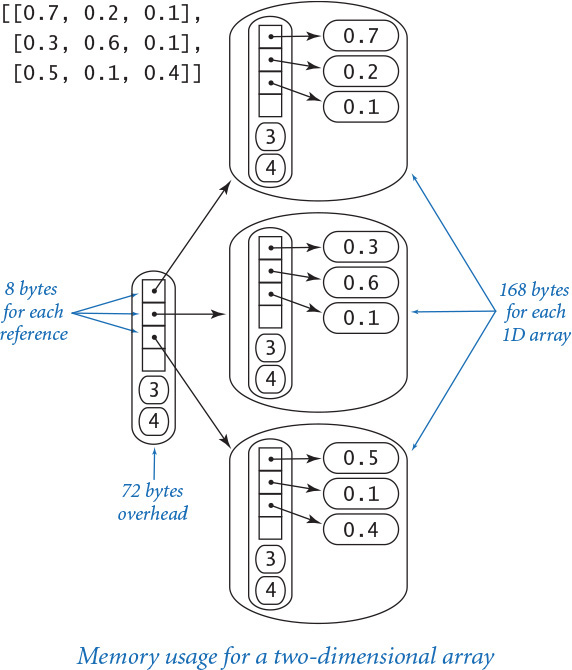
Two-dimensional arrays and arrays of objects
A two-dimensional array is an array of arrays, so we can calculate the memory consumption of a two-dimensional array with m rows and n columns from the information in the previous paragraph. Each row is an array that consumes 72 + 32n bytes, so the total is 72 (overhead) plus 8m (references to the rows) plus m(72 + 32n) (memory for the m rows) bytes, for a grand total of 72 + 80m + 32mn bytes. The same logic works for an array of any type of object: if an object uses x bytes, an array of m such objects consumes a total of 72 + m(x+8) bytes. Again, this is likely to be a slight underestimate because of the resizing array data structure Python uses to represent arrays. Note: Python’s sys.getsizeof(x) is not much help in these calculations because it does not calculate the memory for the objects themselves—it returns 72 + 8m for any array of length m (or any two-dimensional array with m rows).
Objects
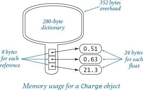
A key question for Python programming is the following: How much memory is required to represent a user-defined object? The answer to this question may surprise you, but is important to know: hundreds of bytes, at least. Specifically, Python uses 72 bytes of overhead plus 280 bytes for a dictionary that binds instance variables to objects (we will discuss dictionaries in SECTION 4.4) plus 24 bytes for a reference to each instance variable plus memory for the instance variables themselves. For example, to represent a Charge object, Python uses at least 72 + 280 = 352 bytes for overhead, 8 * 3 = 24 bytes to store the object references for the three instance variables, 24 bytes to store the float object referenced by the _rx instance variable, 24 bytes to store the float object referenced by the _ry instance variable, and 24 bytes to store the float object referenced by the _q instance variable, for a grand total of (at least) 448 bytes. The total might be even higher on your system, because some implementations consume even more overhead.
These basic mechanisms are effective for estimating the memory usage of a great many programs, but there are numerous complicating factors that can make the task significantly more difficult. For example, we have already noted the potential effect of caching. Moreover, memory consumption is a complicated dynamic process when function calls are involved because the system memory allocation mechanism plays a more important role. For example, when your program calls a function, the system allocates the memory needed for the function (for its local variables) from a special area of memory called the stack, and when the method returns to the caller, this memory is returned to the stack. For this reason, creating arrays or other large objects in recursive functions is dangerous, since each recursive call implies significant memory usage. When you create an object, the system allocates the memory needed for the object from another special area of memory known as the heap. Every object lives until no references to it remain, at which point a system process known as garbage collection reclaims its memory for the heap. Such dynamics can make the task of precisely estimating memory usage of a program challenging.
Despite all these caveats, it is important for every Python programmer to understand that each object of a user-defined type is likely to consume a large amount of memory. So, a Python program that defines a large number of objects of a user-defined type can use much more space (and time) than you might expect. That is especially true if each object contains only a few instance variables—in that case, the ratio of memory devoted to overhead versus memory devoted to instance variables is very high. For example, if you compare the performance of our Complex type with Python’s built-in complex type for mandelbrot.py, you will certainly notice this effect. Numerous object-oriented languages have come and gone since the concept was introduced decades ago, and many of them eventually embraced lightweight objects for user-defined types. Python offers two advanced features for this purpose—named tuples and slots—but we will not take advantage of such memory optimizations in this book.
Perspective
Good performance is important. An impossibly slow program is almost as useless as an incorrect one, so it is certainly worthwhile to pay attention to the cost at the outset, so as to have some idea of what sorts of problems you might feasibly address. In particular, it is always wise to have some idea of which code constitutes the inner loop of your programs.
Perhaps the most common mistake made in programming is to pay too much attention to performance characteristics. Your first priority is to make your code clear and correct. Modifying a program for the sole purpose of speeding it up is best left for experts. Indeed, doing so is often counterproductive, as it tends to create code that is complicated and difficult to understand. C. A. R. Hoare (the inventor of quicksort and a leading proponent of composing clear and correct code) once summarized this idea by saying that “premature optimization is the root of all evil,” to which Knuth added the qualifier “(or at least most of it) in programming.” Beyond that, improving the running time is not worthwhile if the available cost benefits are insignificant. For example, improving the running time of a program by a factor of 10 is inconsequential if the running time is only an instant. Even when a program takes a few minutes to run, the total time required to implement and debug an improved algorithm might be substantially longer than the time required simply to run a slightly slower one—you may as well let the computer do the work. Worse, you might spend a considerable amount of time and effort implementing ideas that do not actually make a program any faster.
Perhaps the second most common mistake made in developing an algorithm is to ignore performance characteristics. Faster algorithms are often more complicated than brute-force solutions, so you might be tempted to accept a slower algorithm to avoid having to deal with more complicated code. However, you can sometimes reap huge savings with just a few lines of good code. Users of a surprising number of computer systems lose substantial time waiting for simple quadratic algorithms to finish solving a problem, even though linear or linearithmic algorithms are available that are only slightly more complicated and could therefore solve the problem in a fraction of the time. When we are dealing with huge problem sizes, we often have no choice but to seek better algorithms.
Improving a program to make it clearer, more efficient, and elegant should be your goal every time that you work on it. If you pay attention to the cost all the way through the development of a program, you will reap the benefits every time you use it.
Q&A
Q. The text notes that operations on very large integers can consume more than constant time. Can you be more precise?
A. Not really. The definition of “very large” is system dependent. For most practical purposes, you can consider operations applied to 32- or 64-bit integers to work in constant time. Modern applications in cryptography involve huge numbers with hundreds or thousands of digits.
Q. How do I find out how long it takes to add or multiply two floats on my computer?
A. Run some experiments! The program timeops.py on the booksite uses Stopwatch to test the execution time of various arithmetic operations on integers and floats. This technique measures the actual elapsed time as would be observed on a wall clock. If your system is not running many other applications, it can produce accurate results. Python also includes the timeit module for measuring the running time of small code fragments.
Q. Is there any way to measure processor time instead of wall clock time?
A. On some systems, the function call time.clock() returns the current processor time as a float, expressed in seconds. When available, you should substitute time.time() with time.clock() for benchmarking Python programs.
Q. How much time do functions such as math.sqrt(), math.log(), and math.sin() take?
A. Run some experiments! Stopwatch makes it easy to compose programs such as timeops.py to answer questions of this sort for yourself. You will be able to use your computer much more effectively if you get in the habit of doing so.
Q. Why does allocating an array (Python list) of size n take time proportional to n?
A. Python initializes all array elements to whatever values the programmer specifies. That is, in Python there is no way to allocate memory for an array without also assigning an object reference to each element of the array. Assigning object references to each element of an array of size n takes time proportional to n.
Q. How do I find out how much memory is available for my Python programs?
A. Since Python will raise a MemoryError when it runs out of memory, it is not difficult to run some experiments. For example, use this program (bigarray.py):
import sys
import stdarray
import stdio
n = int(sys.argv[1])
a = stdarray.create1D(n, 0)
stdio.writeln('finished')
and run it like this:
% python bigarray.py 100000000
finished
to show that you have room for 100 million integers. But if you type
% python bigarray.py 1000000000
Python will hang, crash, or raise a run-time error; you can conclude that you do not have room for an array of 1 billion integers.
Q. What does it mean when someone says that the worst-case running time of an algorithm is O(n2)?
A. That is an example of a notation known as big-O notation. We write f(n) is O(g(n)) if there exist constants c and n0 such that f(n) ≤ c g(n) for all n > n0. In other words, the function f(n) is bounded above by g(n), up to constant factors and for sufficiently large values of n. For example, the function 30n2 + 10n+ 7 is O(n2). We say that the worst-case running time of an algorithm is O(g(n)) if the running time as a function of the input size n is O(g(n)) for all possible inputs. This notation is widely used by theoretical computer scientists to prove theorems about algorithms, so you are sure to see it if you take a course in algorithms and data structures. It provides a worst-case performance guarantee.
Q. So can I use the fact that the worst-case running time of an algorithm is O(n3) or O(n2) to predict performance?
A. No, because the actual running time might be much less. For example, the function 30n2 + 10n+ 7 is O(n2), but it is also O(n3) and O(n10) because big-O notation provides only an upper bound on the worst-case running time. Moreover, even if there is some family of inputs for which the running time is proportional to the given function, perhaps these inputs are not encountered in practice. Consequently, you cannot use big-O notation to predict performance. The tilde notation and order-of-growth classifications that we use are more precise than big-O notation because they provide matching upper and lower bounds on the growth of the function. Many programmers incorrectly use big-O notation to indicate matching upper and lower bounds.
Q. How much memory does Python typically use to store a tuple of n items?
A. 56 + 8n bytes, plus whatever memory is needed for the objects themselves. This is a bit less than for arrays because Python can implement a tuple (at the machine level) using an array instead of a resizing array.
Q. Why does Python use so much memory (280 bytes) to store a dictionary that maps an object’s instance variables to its values?
A. In principle, different objects from the same data type can have different instance variables. In this case, Python would need some way to manage an arbitrary number of possible instance variables for each object. But most Python code does not call for this (and, as a matter of style, we never need it in this book).
Exercises
4.1.1 Implement the function writeAllTriples() for threesum.py, which writes all of the triples that sum to zero.
4.1.2 Modify threesum.py to take a command-line argument x and find a triple of numbers on standard input whose sum is closest to x.
4.1.3 Compose a program foursum.py that reads an integer n from standard input, then reads n integers from standard input, and counts the number of distinct 4-tuples that sum to zero. Use a quadruply nested loop. What is the order of growth of the running time of your program? Estimate the largest n that your program can handle in an hour. Then, run your program to validate your hypothesis.
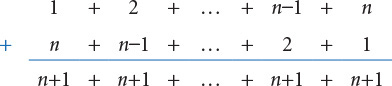
4.1.4 Prove that 1 + 2 + ... + n = n(n+1)/2.
Solution: We proved this by induction at the beginning of SECTION 2.3. Here is the basis for another proof:
4.1.5 Prove by induction that the number of distinct triples of integers between 0 and n–1 is n(n–1)(n–2)/6.
Solution: The formula is correct for n = 2. For n > 2, count all the triples that do not include n, which is (n–1)(n–2)(n–3)/6 by the inductive hypothesis, and all the triples that do include n–1, which is (n–1)(n–2)/2, to get the total
(n–1)(n–2)(n–3)/6 + (n–1)(n–2)/2 = n(n–1)(n–2)/6.
4.1.6 Show by approximating with integrals that the number of distinct triples of integers between 0 and n–1 is about n3/6.
Solution: ![]()
4.1.7 What is the value of x (as a function of n) after running the following code fragment?
x = 0
for i in range(n):
for j in range(i+1, n):
for k in range(j+1, n):
x += 1
Solution: n (n–1) (n–2) / 6.
4.1.8 Use tilde notation to simplify each of the following formulas, and give the order of growth of each:
a. n(n – 1)(n – 2) (n – 3)/24
b. (n – 2) (lg n – 2) (lg n +2)
c. n(n +1) – n2
d. n(n +1)/2 +n lg n
e. ln((n – 1)(n – 2) (n – 3))2
4.1.9 Is the following code fragment linear, quadratic, or cubic (as a function of n)?
for i in range(n):
for j in range(n):
if i == j: c[i][j] = 1.0
else: c[i][j] = 0.0
4.1.10 Suppose the running time of an algorithm on inputs of size 1,000, 2,000, 3,000, and 4,000 is 5 seconds, 20 seconds, 45 seconds, and 80 seconds, respectively. Estimate how long it will take to solve a problem of size 5,000. Is the algorithm linear, linearithmic, quadratic, cubic, or exponential?
4.1.11 Which would you prefer: a quadratic, linearithmic, or linear algorithm?
Solution: While it is tempting to make a quick decision based on the order of growth, it is very easy to be misled by doing so. You need to have some idea of the problem size and of the relative value of the leading coefficients of the running time. For example, suppose that the running times are n2 seconds, 100 n log2 n seconds, and 10,000n seconds. The quadratic algorithm will be fastest for n up to about 1,000, and the linear algorithm will never be faster than the linearithmic one (n would have to be greater than 2100—far too large to bother considering).
4.1.12 Apply the scientific method to develop and validate a hypothesis about order of growth of the running time of the following code fragment, as a function of the argument n:
def f(n):
if (n == 0): return 1
return f(n-1) + f(n-1)
4.1.13 Apply the scientific method to develop and validate a hypothesis about order of growth of the running time of each of the following code fragments as a function of n:
s = ''
for i in range(n):
if stdrandom.bernoulli(0.5): s += '0'
else: s += '1'
s = ''
for i in range(n):
oldS = s
if stdrandom.bernoulli(0.5): s += '0'
else: s += '1'
Solution: On many systems, the first is linear; the second is quadratic. You have no way of knowing why: In the first case, Python detects that s is the only variable that refers to the string, so it appends each character to the string as it would with a list (in amortized constant time) even though the string is immutable! A safer alternative is to create a list containing the characters and concatenate them together with by calling the join() method.
a = []
for i in range(n):
if stdrandom.bernoulli(0.5): a += ['0']
else: a += ['1']
s = ''.join(a)
4.1.14 Each of the four Python functions below returns a string of length n whose characters are all x. Determine the order of growth of the running time of each function. Recall that concatenating two strings in Python takes time proportional to the sum of their lengths.
def f1(n):
if (n == 0):
return ''
temp = f1(n // 2)
if (n % 2 == 0): return temp + temp
else: return temp + temp + 'x'
def f2(n):
s = ''
for i in range(n):
s += 'x'
return s
def f3(n):
if (n == 0): return ''
if (n == 1): return 'x'
return f3(n//2) + f3(n - n//2)
def f4(n):
temp = stdarray.create1D(n, 'x')
return ''.join(temp)
def f5(n):
return 'x' * n
4.1.15 Each of the three Python functions below returns the reverse of a string of length n. What is the order of growth of the running time of each function?
def reverse1(s):
n = len(s)
reverse = ''
for i in range(n):
reverse = s[i] + reverse
return reverse
def reverse2(s):
n = len(s)
if (n <= 1):
return s
left = s[0 : n//2]
right = s[n//2 : n]
return reverse2(right) + reverse2(left)
def reverse3(s):
return s[::-1]
The slice expression s[::-1] uses an optional third argument to specify the step size.
4.1.16 The following code fragment (adapted from a Java programming book) creates a random permutation of the integers from 0 to n–1. Determine the order of growth of its running time as a function of n. Compare its order of growth with the shuffling code in SECTION 1.4.
a = stdarray.create1D(n, 0)
taken = stdarray.create1D(n, False)
count = 0
while (count < n):
r = stdrandom.uniform(0, n)
if not taken[r]:
a[r] = count
taken[r] = True
count += 1
4.1.17 How many times does the following code fragment execute the first if statement in the triply nested loop?
for i in range(n):
for j in range(n):
for k in range(n):
if (i < j) and (j < k):
if a[i] + a[j] + a[k] == 0:
count += 1
Use tilde notation to simply your answer.
4.1.18 Apply the scientific method to develop and validate a hypothesis about order of growth of the running time of the collect() method in coupon.py (PROGRAM 2.1.3), as a function of the argument n. Note: Doubling is not effective for distinguishing between the linear and linearithmic hypotheses—you might try squaring the size of the input.
4.1.19 Apply the scientific method to develop and validate a hypothesis about order of growth of the running time of markov.py (PROGRAM 1.6.3), as a function of the arguments moves and n.
4.1.20 Compose a program mooreslaw.py that takes a command-line argument n and writes the increase in processor speed over a decade if processor speed doubles every n months. How much will processor speed increase over the next decade if speeds double every n = 15 months? 24 months?
4.1.21 Using the memory model from the text, give the memory requirements for each object of the following data types from CHAPTER 3:
a. Stopwatch
b. Turtle
c. Vector
d. Body
e. Universe
4.1.22 Estimate, as a function of the grid size n, the amount of memory used by visualizev.py (PROGRAM 2.4.4) with vertical percolation detection (PROGRAM 2.4.2). Extra credit: Answer the same question for the case where the recursive percolation detection method percolation.py (PROGRAM 2.4.6) is used.
4.1.23 Estimate the size of the largest n-by-n array of integers that your computer can hold, and then try to allocate such an array.
4.1.24 Estimate, as a function of the number of documents n and the dimension d, the amount of space used by comparedocuments.py (PROGRAM 3.3.5).
4.1.25 Compose a version of primesieve.py (PROGRAM 1.4.3) that uses an array of integers instead of an array of booleans and uses 32 bits in each integer, to raise the largest value of n that it can handle by a factor of 32.
4.1.26 The following table gives running times for various programs for various values of n. Fill in the blanks with estimates that you think are reasonable on the basis of the information given.
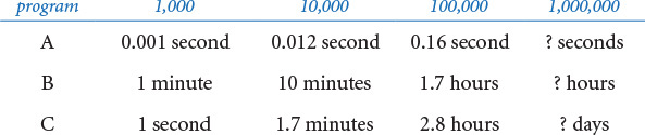
Give hypotheses for the order of growth of the running time of each program.
Creative Exercises
4.1.27 Three-sum analysis. Calculate the probability that no triple among n random 32-bit integers sums to 0, and give an approximate estimate for n equal to 1,000, 2,000, and 4,000. Extra credit: Give an approximate formula for the expected number of such triples (as a function of n), and run experiments to validate your hypothesis.
4.1.28 Closest pair. Design a quadratic algorithm that finds the pair of integers that are closest to each other. (In the next section you will be asked to find a linearithmic algorithm.)
4.1.29 Power law. Show that a log-log plot of the function cnb has slope b and x-intercept log c. What are the slope and x-intercept for 4 n3 (log n)2 ?
4.1.30 Sum furthest from zero. Design an algorithm that finds the pair of integers whose sum is furthest from zero. Can you discover a linear-time algorithm?
4.1.31 The “beck” exploit. A popular web server supports a function no2slash() whose purpose is to collapse multiple / characters. For example, the string /d1///d2////d3/test.html becomes /d1/d2/d3/test.html. The original algorithm was to repeatedly search for a / and copy the remainder of the string:
def no2slash(name):
for x in range(1, len(name)):
if x > 0:
if (name[x-1] == '/') and (name[x] == '/'):
for y in range(x+1, len(name)):
name[y-1] = name[y]
else:
x += 1
Unfortunately, the running time of this code is quadratic in the number of / characters in the input. By sending multiple simultaneous requests with large numbers of / characters, a hacker can deluge a server and starve other processes for CPU time, thereby creating a denial-of-service attack. Develop a version of no2slash() that runs in linear time and does not allow for this type of attack.
4.1.32 Young tableaux. Suppose you have in memory an n-by-n array of integers a[][] such that a[i][j] < a[i+1][j] and a[i][j] < a[i][j+1] for all i and j, like the table below:
5 23 54 67 89
6 69 73 74 90
10 71 83 84 91
60 73 84 86 92
99 91 92 93 94
Devise an algorithm whose order of growth is linear in n to determine whether a given integer x is in a given Young tableaux.
4.1.33 Subset sum. Compose a program anysum.py that takes an integer n from standard input, then reads n integers from standard input, and counts the number of subsets that sum to 0. Give the order of growth of the running time of your program.
4.1.34 Array rotation. Given an array of n elements, give a linear-time algorithm to rotate the array by k positions. That is, if the array contains a0, a1, ..., an-1, the rotated array is ak, ak+1, ..., an-1, a0, ..., ak-1. Use at most a constant amount of extra space (array indices and array values). Hint: Reverse three subarrays.
4.1.35 Finding a duplicated integer. (a) Given an array of n integers from 1 to n with one value repeated twice and one missing, give an algorithm that finds the missing integer, in linear time and constant extra space. (b) Given a read-only array of n integers, where each value from 1 to n–1 occurs once and one occurs twice, give an algorithm that finds the duplicated value, in linear time and constant extra space. (c) Given a read-only array of n integers with values between 1 and n–1, give an algorithm that finds a duplicated value, in linear time and constant extra space.
4.1.36 Factorial. Design a fast algorithm to compute n! for large values of n. Use your program to compute the longest run of consecutive 9s in 1000000!. Develop and validate a hypothesis for the order of growth of the running time of your algorithm.
4.1.37 Maximum sum. Design a linear-time algorithm that finds a contiguous subsequence of at most m in a sequence of n integers that has the highest sum among all such subsequences. Implement your algorithm, and confirm that the order of growth of its running time is linear.
4.1.38 Pattern matching. Given an n-by-n array of black (1) and white (0) pixels, design a linear algorithm that finds the largest square subarray that consists of entirely black pixels. As an example, the following 8-by-8 array contains a 3-by-3 subarray entirely of black pixels:
1 0 1 1 1 0 0 0
0 0 0 1 0 1 0 0
0 0 1 1 1 0 0 0
0 0 1 1 1 0 1 0
0 0 1 1 1 1 1 1
0 1 0 1 1 1 1 0
0 1 0 1 1 0 1 0
0 0 0 1 1 1 1 0
Implement your algorithm and confirm that the order of growth of its running time is linear in the number of pixels. Extra credit: Design an algorithm to find the largest rectangular black subarray.
4.1.39 Maximum average. Compose a program that finds a contiguous subarray of at most m elements in an array of n integers that has the highest average value among all such subarrays, by trying all subarrays. Use the scientific method to confirm that the order of growth of the running time of your program is mn2. Next, compose a program that solves the problem by first computing prefix[i] = a[0] + ... + a[i] for each i, then computing the average in the interval from a[i] to a[j] with the expression (prefix[j] - prefix[i]) / (j - i + 1). Use the scientific method to confirm that this method reduces the order of growth by a factor of n.
4.1.40 Sub-exponential function. Find a function whose order of growth is larger than any polynomial function, but smaller than any exponential function. Extra credit: Compose a program whose running time has that order of growth.
4.1.41 Resizing arrays. For each of the following strategies, either show that each resizing array operation takes constant amortized time or find a sequence of n operations (starting from an empty data structure) that takes quadratic time.
a. Double the capacity of the resizing array when it is full and halve the capacity when it is half full.
b. Double the capacity of the resizing array when it is full and halve the capacity when it is one-third full.
c. Increase the capacity of the resizing array by a factor of 9/8 when it is full and decrease it by a factor of 9/8 when it is 80% full.
4.2 Sorting and Searching
The sorting problem seeks to rearrange an array of elements in ascending order. It is a familiar and critical task in many computational applications: the songs in your music library are in alphabetical order, your email messages are in reverse order of the time received, and so forth. Keeping things in some kind of order is a natural desire. One reason that it is so useful is that it is much easier to search for something in a sorted list than an unsorted one. This need is particularly acute in computing, where the list of things to search can be huge and an efficient search can be an important factor in a problem’s solution.
Sorting and searching are important for commercial applications (businesses keep customer files in order) and scientific applications (to organize data and computation), and have all manner of applications in fields that may appear to have little to do with keeping things in order, including data compression, computer graphics, computational biology, numerical computing, combinatorial optimization, cryptography, and many others.
We use these fundamental problems to illustrate the idea that efficient algorithms are one key to effective solutions for computational problems. Indeed, many different sorting and searching algorithms have been proposed. Which should we use to address a given task? This question is important because different algorithms can have vastly differing performance characteristics, enough to make the difference between success in a practical situation and not coming close to doing so, even on the fastest available computer.
In this section, we will consider in detail two classical algorithms for sorting and searching, along with several applications in which their efficiency plays a critical role. With these examples, you will be convinced not just of the utility of these algorithms, but also of the need to pay attention to the cost whenever you address a problem that requires a significant amount of computation.
Binary search
The game of “twenty questions” (see PROGRAM 1.5.2, twentyquestions.py) provides an important and useful lesson in the idea of designing and using efficient algorithms for computational problems. The setup is simple: your task is to guess the value of a secret number that is one of the n integers between 0 and n – 1. Each time that you make a guess, you are told whether your guess is equal to the secret number, too high, or too low. As we discussed in SECTION 1.5, an effective strategy is to guess the number in the middle of the interval, then use the answer to halve the length of the interval that can contain the secret number. For reasons that will become clear later, we begin by slightly modifying the game to make the questions of the form “Is the number greater than or equal to m?” with only true or false answers, and assume for the moment that n is a power of 2. Now, the basis of an effective algorithm that always gets to the secret number in a minimal number of questions (in the worst case) is to maintain an interval that contains the secret number and shrink it by half at each step. More precisely, we use a half-open interval, which contains the left endpoint but not the right one. We use the notation [l o, hi) to denote all of the integers greater than or equal to lo and less than (but not equal to) hi. We start with lo = 0 and hi = n and use the following recursive strategy:
• Base case: If hi –lo equals 1, then the secret number is lo.
• Recursive step: Otherwise, ask whether the secret number is greater than or equal to the number mid = (hi + lo) / 2. If so, look for the number in [mid, hi); if not, look for the number in [lo, mid).

This strategy is an example of the general problem-solving algorithm known as binary search, which has many applications. PROGRAM 4.2.1 (questions.py) is an implementation.
Program 4.2.1 Binary search (20 questions) (questions.py)
import sys
import stdio
def search(lo, hi):
if (hi - lo) == 1:
return lo
mid = (hi + lo) // 2
stdio.write('Greater than or equal to ' + str(mid) + '? ')
if stdio.readBool():
return search(mid, hi)
else:
return search(lo, mid)
k = int(sys.argv[1])
n = 2 ** k
stdio.write('Think of a number ')
stdio.writeln('between 0 and ' + str(n - 1))
guess = search(0, n)
stdio.writeln('Your number is ' + str(guess))
lo | smallest possible integer
hi - 1 | largest possible integer
mid | midpoint
n | number of possible integers
k | number of questions
This script uses binary search to play the same game as PROGRAM 1.5.2, but with the roles reversed: you choose the secret number and the program guesses its value. It takes a command-line argument k, asks you to think of a number between 0 and 2k–1, and always guesses the answer with k questions.
% python questions.py 7
Think of a number between 0 and 127
Greater than or equal to 64? True
Greater than or equal to 96? False
Greater than or equal to 80? False
Greater than or equal to 72? True
Greater than or equal to 76? True
Greater than or equal to 78? False
Greater than or equal to 77? True
Your number is 77
Correctness proof
First, we have to convince ourselves that the strategy is correct—in other words, that it always leads us to the secret number. We do so by establishing the following facts:
• The interval always contains the secret number.
• The interval lengths are the powers of 2, decreasing from 2k.
The first of these facts is enforced by the code; the second follows by noting that if (hi–lo) is a power of 2, then (hi – lo) / 2 is the next smaller power of 2 and also the length of both halved intervals. These facts are the basis of an induction proof that the algorithm operates as intended. Eventually, the interval length becomes 1, so we are guaranteed to find the number.
Analysis of running time
Let n be the number of possible values. In questions.py, we have n = 2k, where k = lg n. Now, let T(n) be the number of questions. The recursive strategy immediately implies that T(n) must satisfy the following recurrence relation:
T(n) = T(n/2) + 1
with T(1) = 0. Substituting 2k for n, we can telescope the recurrence (apply it to itself) to immediately get a closed-form expression:
T(2k) = T(2k–1) + 1 = T(2k–2) + 2 = ... = T(1) + k = k.
Substituting back n for 2k (and lg n for k) gives the result
T(n) = lg n
We normally use this equation to justify a hypothesis that the running time of a program that uses binary search is logarithmic. Note: Binary search and questions.search() work even when n is not a power of 2 (see EXERCISE 4.2.1).
Linear–logarithmic chasm
The alternative to using binary search is to guess 0, then 1, then 2, then 3, and so forth, until we hit the secret number. We refer to such an algorithm as a brute-force algorithm: it seems to get the job done, but without much regard to the cost (which might prevent it from actually getting the job done for large problems). In this case, the running time of the brute-force algorithm is sensitive to the secret number, but could take as many as n questions in the worst case. Meanwhile, binary search guarantees to take no more than lg n questions (or, more precisely, ⌈lg n⌉ if n is not a power of 2). As you will learn to appreciate, the difference between n and lg n makes a huge difference in practical applications. Understanding the enormity of this difference is a critical step to understanding the importance of algorithm design and analysis. In the present context, suppose that it takes 1 second to process a question. With binary search, you can guess the value of any number less than 1 million in 20 seconds; with the brute-force algorithm, it might take 1 million seconds, which is more than 1 week. We will see many examples where such a cost difference is the determining factor in whether a practical problem can be feasibly solved.
Binary representation
If you look back to PROGRAM 1.3.7 (binary.py), you will immediately recognize that binary search is nearly the same computation as converting a number to binary! Each question determines one bit of the answer. In our example, the information that the number is between 0 and 127 says that the number of bits in its binary representation is 7, the answer to the first question (Is the number greater than or equal to than 64?) tells us the value of the leading bit, the answer to the second question tells us the value of the next bit, and so forth. For example, if the number is 77, the sequence of answers True False False True True False True immediately yields 1001101, the binary representation of 77.
Thinking in terms of the binary representation is another way to understand the linear–logarithmic chasm: when we have a program whose running time is linear in a parameter n, its running time is proportional to the value of n, whereas a logarithmic running time is just proportional to the number of digits in n. In a context that is perhaps slightly more familiar to you, think about the following question, which illustrates the same point: would you rather earn $6 or a six-figure salary?
Inverting a function
As an example of the utility of binary search in scientific computing, we revisit a problem that we first encountered in SECTION 2.1: inverting an increasing function (see EXERCISE 2.1.26). Given an increasing function f and a value y, and an open interval (lo, hi), our task is to find a value x within the interval such that f(x) = y. In this situation, we use real numbers as the endpoints of our interval, not integers, but we use the same essential approach that we used for guessing a hidden integer with the “twenty questions” problem: we halve the length of the interval at each step, keeping x in the interval, until the interval is sufficiently small that we know the value of x to within a desired precision δ, which we take as an argument to the function. The figure at the top of the next page illustrates the first step.

PROGRAM 4.2.2 (bisection.py) implements this strategy. We start with an interval (lo, hi) known to contain x and use the following recursive procedure:
• Compute mid = (hi + lo) / 2.
• Base case: If hi – lo is less than δ, then return mid as an estimate of x.
• Recursive step: Otherwise, test whether f(mid) > y. If so, look for x in (lo, mid); if not, look for x in (mid, hi).
The key to this approach is the idea that the function is increasing—for any values a and b, knowing that f(a) < f(b) tells us that a < b, and vice versa. The recursive step just applies this knowledge: knowing that y = f(x) < f(mid) tells us that x < mid, so that x must be in the interval (lo, mid), and knowing that y = f(x) > f(mid) tells us that x > mid, so that x must be in the interval (mid, hi). You can think of the problem as determining which of the n = (hi–l o) / δ tiny intervals of length δ within (lo, hi) contains x, with running time logarithmic in n. As with converting an integer to binary, we determine one bit of x in each iteration. In this context, binary search is often called bisection search because we bisect the interval at each stage.
Weighing an object
Binary search has been known since antiquity, perhaps partly because of the following application. Suppose that you need to determine the weight of a given object using only a balancing scale. With binary search, you can do so with weights that are powers of 2 (and just one weight of each type). Put the object on the right side of the balance and try the weights in decreasing order on the left side. If a weight causes the balance to tilt to the left, remove it; otherwise, leave it. This process is precisely analogous to determining the binary representation of a number by subtracting decreasing powers of 2, as in PROGRAM 1.3.7.
Program 4.2.2 Bisection search (bisection.py)
import sys
import stdio
import gaussian
def invert(f, y, lo, hi, delta=0.00000001):
mid = (lo + hi) / 2.0
if (hi - lo) < delta:
return mid
if f(mid) > y:
return invert(f, y, lo, mid, delta)
else:
return invert(f, y, mid, hi, delta)
def main():
y = float(sys.argv[1])
x = invert(gaussian.cdf, y, -8.0, 8.0)
stdio.writef('%.3f
', x)
if __name__ == '__main__': main()
f | function
y | given value
delta | precision
lo | left endpoint
mid | midpoint
hi | right endpoint
The function invert() in this program uses binary search to compute a float x within the interval (lo, hi) for which f(x) is equal to a given value y, within a given precision delta, for any function f that is increasing in the interval. It is a recursive function that halves the interval containing the given value, evaluates the function at the midpoint of the interval, and decides whether the desired float x is in the left half or the right half, continuing until the interval length is less than the given precision.
% python bisection.py .5
0.000
% python bisection.py .95
1.645
% python bisection.py .975
1.960

Binary search in a sorted array
One of the most important uses of binary search is to find a piece of information using a key to guide the search. This usage is ubiquitous in modern computing, to the extent that printed artifacts that depend on the same concepts are well on their way to becoming obsolete. For example, during the last few centuries, people would use a publication known as a dictionary to look up the definition of a word, and during much of the last century people would use a publication known as a phone book to look up a person’s phone number. In both cases, the basic mechanism is the same: entries appear in order, sorted by a key that identifies it (the word in the case of the dictionary, and the person’s name in the case of the phone book, sorted in alphabetical order in both cases). You probably use your computer to reference such information, but think about how you would look up a word in a dictionary. A brute-force solution known as sequential search is to start at the beginning, examine each key one at a time, and continue until you find the word. No one uses that approach: instead, you open the book to some interior page and look for the word on that page. If it is there, you are done; otherwise, you eliminate either the part of the book before the current page or the part of the book after the current page from consideration, and then repeat. We now recognize this approach as binary search. Whether you look exactly in the middle is immaterial; as long as you eliminate at least a constant fraction of the keys each time that you look, your search will be logarithmic.
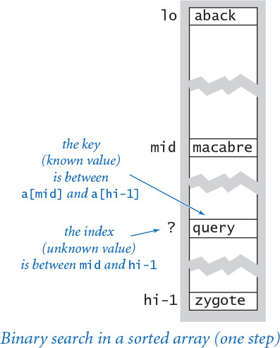
Exception filter
We will consider in SECTION 4.3 the details of implementing the kind of computer program that you use in place of a dictionary or a phone book. PROGRAM 4.2.3 (binarysearch.py) uses binary search to solve the simpler existence problem: is a given key in a sorted array of keys, in any location? For example, when checking the spelling of a word, you need to know only whether your word is in the dictionary and are not interested in the definition. In a computer search, we keep the information in an array, sorted in order of the key (for some applications, the information comes in sorted order; for others, we have to sort it first, using one of the algorithms discussed later in this section). The binary search in binarysearch.py differs from our other applications in two details. First, the array length n need not be a power of 2. Second, it has to allow for the possibility that the key sought is not in the array. Coding binary search to account for these details requires some care, as discussed in this section’s Q&A and exercises.
Program 4.2.3 Binary search (in a sorted array) (binarysearch.py)
import sys
import stdio
from instream import InStream
def _search(key, a, lo, hi):
if hi <= lo: return -1 # Not found.
mid = (lo + hi) // 2
if a[mid] > key:
return _search(key, a, lo, mid)
elif a[mid] < key:
return _search(key, a, mid+1, hi)
else:
return mid
def search(key, a):
return _search(key, a, 0, len(a))
def main():
instream = InStream(sys.argv[1])
a = instream.readAllStrings()
while not stdio.isEmpty():
key = stdio.readString()
if search(key, a) < 0: stdio.writeln(key)
if __name__ == '__main__': main()
key | key sought
a[] | sorted array
lo | smallest possible index
mid | midpoint
hi | largest possible index
The search() method uses binary search to find the index of a key in a sorted array (or returns -1 if the key is not in the array). The test client is an exception filter that reads a sorted array of strings from the whitelist file given on the command line and writes the words from standard input that are not in the whitelist.
% more emails.txt
bob@office
carl@beach
marvin@spam
bob@office
bob@office
mallory@spam
dave@boat
eve@airport
alice@home
% more white.txt
alice@home
bob@office
carl@beach
dave@boat
% python binarysearch.py white.txt < emails.txt
marvin@spam
mallory@spam
eve@airport
The test client in binarysearch.py is known as an exception filter: it reads in a sorted array of strings from a file (which we refer to as the whitelist) and an arbitrary sequence of strings from standard input, and writes those in the sequence that are not in the whitelist. Exception filters have many direct applications. For example, if the whitelist is the words from a dictionary and standard input is a text document, the exception filter will write the misspelled words. Another example arises in web applications: your email application might use an exception filter to reject any messages that are not on a whitelist that contains the email addresses of your friends, or your operating system might have an exception filter that disallows network connections to your computer from any device having an IP address that is not on a preapproved whitelist.
Fast algorithms are an essential element of the modern world, and binary search is a prototypical example that illustrates the impact of fast algorithms. Whether it be extensive experimental data or detailed representations of some aspect of the physical world, modern scientists are awash in vast amounts of data. With a few quick calculations, you can convince yourself that problems like finding all the misspelled words in a document or protecting your computer from intruders using an exception filter require a fast algorithm like binary search. Take the time to do so—a fast algorithm can certainly make the difference between being able to solve a problem easily and spending substantial resources trying to do so (and failing). You can find the exceptions in a million-word document to a million-entry whitelist in an instant, whereas that task might take days or weeks using the brute-force algorithm. Nowadays, web companies routinely provide services that are based on using binary search billions of times in arrays with billions of elements—without a fast algorithm like binary search, we could not contemplate such services.
Insertion sort
Binary search requires that the array be sorted, and sorting has many other direct applications, so we now turn to sorting algorithms. We consider first a brute-force algorithm, then a sophisticated algorithm that we can use for huge arrays.
The brute-force algorithm we consider is known as insertion sort. It is based on a simple approach that people often use to arrange hands of playing cards—that is, consider the cards one at a time and insert each into its proper place among those already considered (keeping them sorted).
PROGRAM 4.2.4 (insertion.py) contains an implementation of a sort() function that mimics this process to sort elements in an array a[] of length n. The test client reads all the strings from standard input, puts them into the array, calls the sort() function to sort them, and then writes the sorted result to standard output.
In insertion.sort(), the outer for loop sorts the first i elements in the array. The inner while loop completes the sort by putting a[i] into its proper position in the array, as in the following example when i is 6:

Element a[i] is put in its place among the sorted elements to its left by exchanging it (using a tuple-packing variant of the exchange() function that we first encountered in SECTION 2.1) with each larger element to its left, moving from right to left, until it reaches its proper position. The black elements in the three bottom rows in this trace are the ones that are compared (and exchanged, on all but the final iteration).
The insertion process just described is executed first with i equal to 1, then 2, then 3, and so forth, as illustrated in the trace at the top of the next page. When i reaches the end of the array, the whole array is sorted.
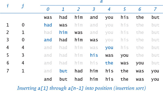
This trace displays the contents of the array each time the outer for loop completes, along with the value of j at that time. The highlighted element is the one that was in a[i] at the beginning of the loop, and the other elements printed in black are the other ones that were involved in exchanges and moved to the right one position within the loop. Since the elements a[0] through a[i-1] are in sorted order when the loop completes for each value of i, they are, in particular, in sorted order the final time the loop completes, when the value of i is len(a). This discussion again illustrates the first thing that you need to do when studying or developing a new algorithm: convince yourself that it is correct. Doing so provides the basic understanding that you need to study its performance and use it effectively.
Analysis of running time
The sort() function contains a while loop nested inside a for loop, which suggests that the running time is quadratic. However, we cannot immediately draw this conclusion because the while loop terminates as soon as a[j] is greater than or equal to a[j-1]. For example, in the best case, when the argument array is already in sorted order, the while loop amounts to nothing more than a comparison (to learn that a[j] is greater than or equal to a[j-1] for each j from 1 to n-1), so the total running time is linear. On the other hand, if the argument array is in reverse-sorted order, the while loop does not terminate until j equals 0. So, the frequency of execution of the instructions in the inner loop is
1 + 2 + ... + n–1 ~ n2 /2
Program 4.2.4 Insertion sort (insertion.py)
import sys
import stdio
def exchange(a, i, j):
a[i], a[j] = a[j], a[i]
def sort(a):
n = len(a)
for i in range(1, n):
j = i
while (j > 0) and (a[j] < a[j-1]):
exchange(a, j, j-1)
j -= 1
def main():
a = stdio.readAllStrings()
sort(a)
for s in a:
stdio.write(s + ' ')
stdio.writeln()
if __name__ == '__main__': main()
a[] | array to sort
n | number of elements
This program reads strings from standard input, sorts them into increasing order, and writes them to standard output. The sort() function is an implementation of insertion sort. It sorts arrays of any type of data that supports < (implements a __lt__() method). Insertion sort is appropriate for small arrays or for large arrays that are nearly in order, but is too slow to use for large arrays that are out of order.
% more tiny.txt
was had him and you his the but
% python insertion.py < tiny.txt
and but had him his the was you
% python insertion.py < TomSawyer.txt
tick tick tick tick tick tick tick tick tick tick tick tick tick tick tick tick tick tick tick tick tick tick tick tick
tick tick tick tick tick tick tick tick tick tick tick tick tick tick tick tick tick tick tick tick tick tick tick tick
and the running time is quadratic (see EXERCISE 4.1.4). To understand the performance of insertion sort for randomly ordered arrays, take a careful look at the trace: it is an n-by-n array with one black element corresponding to each exchange. That is, the number of black elements is the frequency of execution of instructions in the inner loop. We expect that each new element to be inserted is equally likely to fall into any position, so that element will move halfway to the left on average. Thus, on the average, we expect only about one-half the elements below the diagonal (about n2/4 in total) to be black. This observation leads immediately to the hypothesis that the expected running time of insertion sort for a randomly ordered array is quadratic.

Empirical analysis
PROGRAM 4.2.5 (timesort.py) provides the functions that we need to test our hypothesis that insertion sort is quadratic for randomly ordered arrays by running a doubling test (see SECTION 4.1). The module includes two function: timeTrials(), which runs experiments for a given problem size n, and doublingTest(), which computes the ratios of running times between problems of size n/2 and n. We can also use these functions for other sorting algorithms. For insertion sort, the interactive Python session ratio converges to 4, which validates the hypothesis that the running time is quadratic, as discussed in the last section. You are encouraged to run timesort.py on your own computer. As usual, you might notice the effect of caching or some other system characteristic for some values of n, but the quadratic running time should be quite evident, and you will be quickly convinced that insertion sort is too slow to be useful for large inputs.
Sensitivity to input
Note that each function in timesort.py takes an argument trials and runs trials experiments for each problem size, not just one. As we have just observed, one reason for doing so is that the running time of insertion sort is sensitive to its input values. This behavior is quite different from (for example) threesum.py, and it means that we have to carefully interpret the results of our analysis. It is not correct to flatly predict that the running time of insertion sort will be quadratic, because your application might involve input for which the running time is linear. When an algorithm’s performance is sensitive to input values, you might not be able to make accurate predictions without taking the input values into account. We will return to this issue often as we face real applications. Are the strings that we need to sort in random order? Indeed, that is often not the case. In particular, if only a few elements in a large array are out of position, then insertion sort is the method of choice.
Program 4.2.5 Doubling test for sorts (timesort.py)
import stdio
import stdrandom
import stdarray
from stopwatch import Stopwatch
def timeTrials(f, n, trials):
total = 0.0
a = stdarray.create1D(n, 0.0)
for t in range(trials):
for i in range(n):
a[i] = stdrandom.uniformFloat(0.0, 1.0)
watch = Stopwatch()
f(a)
total += watch.elapsedTime()
return total
def doublingTest(f, n, trials):
while True:
prev = timeTrials(f, n // 2, trials)
curr = timeTrials(f, n, trials)
ratio = curr / prev
stdio.writef('%7d %4.2f
', n, ratio)
n *= 2
f() | function to test
n | problem size
trials | number of trials
total | total elapsed time
a[] | array to sort
watch | stopwatch
n | problem size
prev | running time for n // 2
curr | running time for n
ratio | ratio of running times
The function timeTrials() runs the function f() for arrays of n random floats, performing this experiment trials times. Multiple trials produce more accurate results because they dampen system effects and dependence on the input. The function doublingTest() performs a doubling test starting at n, doubling n, and writing the ratio of the time for the current n and the time for the previous n each time through the loop.
% python
>>> import insertion
>>> import timesort
>>> timesort.doublingTest(insertion.sort, 128, 100)
128 3.90
256 3.93
512 3.98
1024 4.12
2048 4.13
Comparable keys
We want to be able to sort any type of data that has a natural order. In a scientific application, we may wish to sort experimental results by numeric values; in a commercial application, we may wish to use monetary amounts, times, or dates; in systems software, we might wish to use IP addresses or account numbers.
Happily, our insertion sort and binary search functions work not only with strings but also with any data type that is comparable. Recall from SECTION 3.3 that a data type is comparable if it implements the six comparison methods and they define a total order. Python’s built-in int, float, and str types are all comparable.
You can make a user-defined type comparable by implementing the six special methods corresponding to the <, <=, ==, !=, >=, and > operators. In fact, our insertion sort and binary search functions rely on only the < operator, but it is better style to implement all six special methods.
A more general design is sometimes appropriate for user-defined types. For example, a teacher might wish to sort a file of student grade records by name on some occasions and by grade on some other occasions. One solution that is often used to handle such situations is to pass the function that is to be used to compare keys as an argument to the sort function.
It is more likely than not in natural applications that the running time of insertion sort is quadratic, so we need to consider faster sorting algorithms. As we know from SECTION 4.1, a back-of-the-envelope calculation can tell us that having a faster computer is not much help. A dictionary, a scientific database, or a commercial database can contain billions of elements; how can we sort such a large array? Next, we turn to a classic algorithm for addressing this question.
Mergesort
To develop a faster sorting method, we use recursion (as we did for binary search) and a divide-and-conquer approach to algorithm design that every programmer needs to understand. This nomenclature refers to the idea that one way to solve a problem is to divide it into independent parts, conquer them independently, and then use the solutions for the parts to develop a solution for the full problem. To sort an array of comparable keys with this strategy, we divide it into two halves, sort the two halves independently, and then merge the results to sort the full array. This method is known as mergesort.

We process contiguous subarrays of a given array, using the notation a [lo, hi) to refer to a[lo], a[lo+1], ..., a[hi–1], (adopting the same convention as we used for binary search to denote a half-open interval that excludes a[hi]). To sort a[lo, hi), we use the following recursive strategy:
• Base case: If the length of the subarray is 0 or 1, it is already sorted.
• Recursive step: Otherwise, compute mid = (hi + lo) / 2, sort (recursively) the two subarrays a [lo, mid) and a [mid, hi), and merge them.
PROGRAM 4.2.6 (merge.py) is an implementation of this algorithm. The array elements are rearranged by the code that follows the recursive calls, which merges the two halves of the array that were sorted by the recursive calls. As usual, the easiest way to understand the merge process is to study a trace of the contents of the array during the merge. The code maintains one index i into the first half, another index j into the second half, and a third index k into an auxiliary array aux[] that holds the result. The merge implementation is a single loop that sets aux[k] to either a[i] or a[j] (and then increments k and the index for the value that is used). If either i or j has reached the end of its subarray, aux[k] is set from the other; otherwise, it is set to the smaller of a[i] or a[j]. After all of the elements from the two halves have been copied to aux[], the sorted result is copied back to the original array. Take a moment to study the trace just given to convince yourself that this code always properly combines the two sorted subarrays to sort the full array.

Program 4.2.6 Mergesort (merge.py)
import sys
import stdio
import stdarray
def _merge(a, lo, mid, hi, aux):
n = hi - lo
i = lo
j = mid
for k in range(n):
if i == mid: aux[k] = a[j]; j += 1
elif j == hi: aux[k] = a[i]; i += 1
elif a[j] < a[i]: aux[k] = a[j]; j += 1
else: aux[k] = a[i]; i += 1
a[lo:hi] = aux[0:n]
def _sort(a, lo, hi, aux):
n = hi - lo
if n <= 1: return
mid = (lo + hi) // 2
_sort(a, lo, mid, aux)
_sort(a, mid, hi, aux)
_merge(a, lo, mid, hi, aux)
def sort(a):
n = len(a)
aux = stdarray.create1D(n)
_sort(a, 0, n, aux)
a[lo, hi) | subarray to sort
n | length of subarray
mid | midpoint
aux[] | extra array for merge
% python merge.py < tiny.txt
was had him and you his the but
had was
and him
and had him was
his you
but the
but his the you
and but had him his the was you
The sort() function in this module is a fast function that you can use to sort arrays of any comparable data type. It is based on a recursive sort() that sorts a[lo, hi) by sorting its two halves recursively, then merging together the two halves to create the sorted result. The output at right is a trace of the sorted subarray for each call to sort() (see EXERCISE 4.2.8). In contrast to insertion.sort(), merge.sort() is suitable for sorting huge arrays.
The recursive method ensures that the two halves of the array are put into sorted order before the merge. Again, the best way to gain an understanding of this process is to study a trace of the contents of the array each time the recursive sort() method returns. Such a trace for our example is shown next. First a[0] and a[1] are merged to make a sorted subarray in a[0, 2), then a[2] and a[3] are merged to make a sorted subarray in a[2, 4), then these two subarrays of size 2 are merged to make a sorted subarray in a[0, 4), and so forth. If you are convinced that the merge works properly, you need only convince yourself that the code properly divides the array to be convinced that the sort works correctly. Note that when the number of elements is not even, the left half will have one fewer element than the right half.

Analysis of running time
The inner loop of mergesort is centered on the auxiliary array. The for loop involves n iterations, so the frequency of execution of the instructions in the inner loop is proportional to the sum of the subarray lengths over all calls to the recursive function. The value of this quantity emerges when we arrange the calls on levels according to their size. For simplicity, suppose that n is a power of 2, with n = 2k. On the first level, we have one call for size n; on the second level, we have two calls for size n/2; on the third level, we have four calls for size n/4; and so forth, down to the last level with n/2 calls of size 2. There are precisely k = lg n levels, giving the grand total n lg n for the frequency of execution of the instructions in the inner loop of mergesort. This equation justifies a hypothesis that the running time of mergesort is linearithmic. Note: When n is not a power of 2, the subarrays on each level are not necessarily all the same size, but the number of levels is still logarithmic, so the linearithmic hypothesis is justified for all n (see EXERCISES 4.2.14 and 4.2.15). The interactive Python script at left uses timesort.doublingTest() (see PROGRAM 4.2.5) to validate this hypotheses.

% python
...
>>> import merge
>>> import timesort
>>> timesort.doublingTest(
... merge.sort, 1024, 100)
1024 1.92
2048 2.19
4096 2.07
8192 2.13
16384 2.13
32768 2.11
65536 2.31
131072 2.14
262144 2.29
524288 2.13
1048576 2.17
You are encouraged to run these tests on your computer. If you do so, you certainly will appreciate that merge.sort() is much faster for large arrays than is insertion.sort() and that you can sort huge arrays with relative ease. Validating the hypothesis that the running time is linearithmic (and not linear) is a bit more work, but you certainly can see that mergesort scales, making it possible for us to address sorting problems that we could not contemplate solving with a brute-force algorithm such as insertion sort.
Quadratic–linearithmic chasm
The difference between n2 and n log n makes a huge difference in practical applications, just as with the linear–logarithmic chasm that is overcome by binary search. Understanding the enormity of this difference is another critical step to understanding the importance of the design and analysis of algorithms. For a great many important computational problems, a speedup from quadratic to linearithmic—such as we achieve with mergesort over insertion sort—makes the difference between the ability to solve a problem involving a huge amount of data and not being able to effectively address it at all.
Python system sort
Python includes two operations for sorting. The method sort() in the built-in list data type rearranges the items in the underlying list into ascending order, much like merge.sort(). In contrast, the built-in function sorted() leaves the underlying list alone; instead, it returns a new list containing the items in ascending order. The interactive Python script at right illustrates both techniques. The Python system sort uses a version of mergesort:. It is likely to be substantially faster (10–20×) than merge.py because it uses a low-level implementation that is not composed in Python, thereby avoiding the substantial overhead that Python imposes on itself. As with our sorting implementations, you can use the system sort with any comparable data type, such as Python’s built-in str, int, and float data types.
% python
...
>>> a = [3, 1, 4, 1, 5]
>>> b = sorted(a)
>>> a
[3, 1, 4, 1, 5]
>>> b
[1, 1, 3, 4, 5]
>>> a.sort()
>>> a
[1, 1, 3, 4, 5]
Mergesort traces back to john von Neumann, an accomplished physicist, who was among the first to recognize the importance of computation in scientific research. Von Neumann made many contributions to computer science, including a basic conception of the computer architecture that has been used since the 1950s. When it came to applications programming, von Neumann recognized that:
• Sorting is an essential ingredient in many applications.
• Quadratic algorithms are too slow for practical purposes.
• A divide-and-conquer approach is effective.
• Proving programs correct and knowing their cost is important.
Computers are many orders of magnitude faster and have many orders of magnitude more memory, but these basic concepts remain important today. People who use computers effectively and successfully know, as did von Neumann, that brute-force algorithms are often only a start. That Python and other modern systems still use von Neumann’s method is testimony to the power of these ideas.
Application: frequency counts
PROGRAM 4.2.7 (frequencycount.py) reads a sequence of strings from standard input and writes to standard output a table of the distinct strings found and the number of times each was found, in decreasing order of frequency. This computation is useful in numerous applications: a linguist might be studying patterns of word usage in long texts, a scientist might be looking for frequently occurring events in experimental data, a merchant might be looking for the customers who appear most frequently in a long list of transactions, or a network analyst might be looking for the heaviest users. Each of these applications might involve millions of strings or more, so we need a linearithmic algorithm (or better). PROGRAM 4.2.7 accomplishes this by performing two sorts.
Computing the frequencies
Our first step is to read the strings from standard input and sort them. In this case, we are not so much interested in the fact that the strings are put into sorted order, but in the fact that sorting brings equal strings together. If the input is
to be or not to be to
then the result of the sort is
be be not or to to to
with equal strings, such as the two occurrences of be and the three occurrences of to, brought together in the array. Now, with equal strings all together in the array, we can make a single pass through the array to compute all of the frequencies. The Counter data type (PROGRAM 3.3.2) is the perfect tool for the job. Recall that a Counter has a string instance variable (initialized to the constructor argument), a count instance variable (initialized to 0), and an increment() method, which increments the counter by 1. We maintain a Python list zipf[] of Counter objects and do the following for each string:
• If the string is not equal to the previous one, create a new Counter and append it to the end of zipf[].
• Increment the most recently created Counter.

At the end of this process, zipf[i] contains the ith string and its frequency.
Program 4.2.7 Frequency counts (frequencycount.py)
import sys
import stdio
from counter import Counter
words = stdio.readAllStrings()
words.sort() # or merge.sort(words)
zipf = []
for i in range(len(words)):
if (i == 0) or (words[i] != words[i-1]):
entry = Counter(words[i], len(words))
zipf += [entry]
zipf[len(zipf) - 1].increment()
zipf.sort() # or merge.sort(zipf)
zipf.reverse()
for entry in zipf:
stdio.writeln(entry)
words | strings in input
zipf[] | counter array
This program sorts the words on standard input, uses the sorted array to count the frequency of occurrence of each, and then sorts the frequencies. The test file used below has over 20 million words. The plot compares the ith frequency relative to the first (bars) with 1/i (blue). This program assumes that the Counter data type is comparable (see PROGRAM 3.3.2 and page 476).
% python frequencycount.py < leipzig.txt
1160105 the
593492 of
560945 to
472819 a
435866 and
430484 in
205531 for
192296 The
188971 that
172225 is
148915 said
147024 on
...

Sorting the frequencies
Next, we sort the Counter objects by frequency. We can do so in client code by augmenting the Counter data type to include the six comparison methods for comparing Counter objects by their counts, as on page 476. Thus, we simply sort the array of Counter objects to rearrange them in ascending order of frequency! Next, we reverse the array so that the elements are in descending order of frequency. Finally, we write each Counter object to standard output. As usual, Python automatically calls the built-in str() function to do so, which, for Counter objects, writes the count followed by the string.
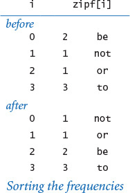
Zipf’s law
The application highlighted in frequencycount.py is elementary linguistic analysis: which words appear most frequently in a text? A phenomenon known as Zipf’s law says that the frequency of the i th most frequent word in a text of m distinct words is proportional to 1/i (with its constant of proportionality being the mth harmonic number). For example, the second most common word should appear about half as often as the first. This is an empirical hypothesis that holds in a surprising variety of situations, ranging from financial data to web usage statistics. The test client run in PROGRAM 4.2.7 validates Zipf’s law for a database containing 1 million sentences drawn from the web (see the booksite).
You are likely to find yourself composing a program sometime in the future for a simple task that could easily be solved by first using a sort. With a linearithmic sorting algorithm such as mergesort, you can address such problems even for huge data sets. PROGRAM 4.2.7 (frequencycount.py), which uses two different sorts, is a prime example. Without a good algorithm (and an understanding of its performance characteristics), you might find yourself frustrated by the idea that your fast and expensive computer cannot solve a problem that seems to be a simple one. With an ever-increasing set of problems that you know how to solve efficiently, you will find that your computer can be a much more effective tool than you now imagine.
Lessons
The vast majority of programs that we compose involve managing the complexity of addressing a new practical problem by developing a clear and correct solution, breaking the program into modules of manageable size, and making use of the basic available resources. From the very start, our approach in this book has been to develop programs along these lines. But as you become involved in ever more complex applications, you will find that a clear and correct solution is not always sufficient, because the cost of computation can be a limiting factor. The examples in this section are a basic illustration of this fact.
Respect the cost of computation
If you can quickly solve a small problem with a simple algorithm, fine. But if you need to address a problem that involves a large amount of data or a substantial amount of computation, you need to take into account the cost. For insertion sort, we did a quick analysis to determine that the brute-force method is infeasible for large arrays.
Divide-and-conquer algorithms
It is worthwhile for you to reflect a bit on the power of the divide-and-conquer paradigm, as illustrated by developing a logarithmic search algorithm (binary search) and a linearithmic sorting algorithm (mergesort). The same basic approach is effective for many important problems, as you will learn if you take a course on algorithm design. For the moment, you are particularly encouraged to study the exercises at the end of this section, which describe problems for which divide-and-conquer algorithms provide feasible solutions and which could not be addressed without such algorithms.
Reduction to sorting
We say that problem A reduces to problem B if we can use a solution to B to solve A. Designing a new divide-and-conquer algorithm from scratch is sometimes akin to solving a puzzle that requires some experience and ingenuity, so you may not feel confident that you can do so at first. But it is often the case that a simpler approach is effective: given a new problem that lends itself to a quadratic brute-force solution, ask yourself how you would solve it if the data were sorted. Often, a relatively simple linear pass through the sorted data will do the job. Thus, we get a linearithmic algorithm, with the ingenuity hidden in the mergesort implementation. For example, consider the problem of determining whether every element in an array has a distinct value. This problem reduces to sorting because we can sort the array, and then pass through the sorted array to check whether the value of any element is equal to the next—if not, they are all distinct.
Know your underlying tools
Our ability to count word frequencies for huge texts using frequencycount.py (PROGRAM 4.2.7) depends on the performance characteristics of the particular operations that we use on arrays and lists. First, its efficiency depends on the fact that mergesort can sort an array in linearithmic time. Second, the efficiency of creating zipf[] depends on the fact that building a list in Python by repeatedly appending items one at time takes time and space linear in the length of the resulting list. This is made possible by the resizing array data structure that Python uses (which we examined in SECTION 4.1). As an applications programmer you must be vigilant, because not all programming languages support such an efficient implementation of appending an item to a list (and performance characteristics are rarely stated in APIs).
Since the advent of computing, people have been developing algorithms such as binary search and mergesort that can efficiently solve practical problems. The field of study known as design and analysis of algorithms encompasses the study of design paradigms like divide-and-conquer, techniques to develop hypotheses about algorithms’ performance, and algorithms for solving fundamental problems like sorting and searching that can be put to use for practical applications of all kinds. Implementations of many of these algorithms are found in Python libraries or other specialized libraries, but understanding these basic tools of computation is like understanding the basic tools of mathematics or science. You can use a matrix-processing package to find the eigenvalues of a matrix, but you still need a course in linear algebra to apply the concepts and interpret the results. Now that you know that a fast algorithm can make the difference between spinning your wheels and properly addressing a practical problem, you can be on the lookout for situations where efficient algorithms like binary search and mergesort can do the job or opportunities where algorithm design and analysis can make the difference.
A. To spare ourselves considerable pain. Binary search is a notable example. For example, you now understand binary search; a classic programming exercise is to compose a version that uses a while loop instead of recursion. Try solving EXERCISES 4.2.1–3 without looking back at the code in the book. In a famous experiment, Jon Bentley once asked several professional programmers to do so, and most of their solutions were not correct.
Q. Why introduce the mergesort algorithm when Python provides an efficient sort() method defined in the list data type?
A. As with many topics we have studied, you will be able to use such tools more effectively if you understand the background behind them.
Q. What is the running time of the following version of insertion sort on an array that is already sorted?
def sort(a):
n = len(a)
for i in range(1, n):
for j in range(i, 0, -1):
if a[j] < a[j-1]: exchange(a, j, j-1)
else: break
A. Quadratic time in Python 2; linear time in Python 3. The reason is that, in Python 2, range() is a function that returns an array of integers of length equal to the length of the range (which can be wasteful if the loop terminates early because of a break or return statement). In Python 3, range() returns an iterator, which generates only as many integers as needed.
Q. What happens if I try to sort an array of elements that are not all of the same type?
A. If the elements are of compatible types (such as int and float), everything works fine. For example, mixed numeric types are compared according to their numeric value, so 0 and 0.0 are treated as equal. If the elements are of incompatible types (such as str and int), then Python 3 raises a TypeError at run time. Python 2 supports some mixed-type comparisons, using the name of the class to determine which object is smaller. For example, Python 2 treats all integers as less than all strings because 'int' is lexicographically less than 'str'.
Q. Which order is used when comparing strings with operators such as == and < ?
A. Informally, Python uses lexicographic order to compare two strings, as words in a book index or dictionary. For example 'hello' and 'hello' are equal, 'hello' and 'goodbye' are unequal, and 'goodbye' is less than 'hello'. More formally, Python first compares the first character of each string. If those characters differ, then the strings as a whole compare as those two characters compare. Otherwise, Python compares the second character of each string. If those characters differ, then the strings as a whole compare as those two characters compare. Continuing in this manner, if Python reaches the ends of the two strings simultaneously, then it considers them to be equal. Otherwise, it considers the shorter string to be the smaller one. Python uses Unicode for character-by-character comparisons. We list a few of the most important properties:
• '0' is less than '1', and so forth.
• 'A' is less than 'B', and so forth.
• 'a' is less than 'b', and so forth.
• Decimal digits ('0' to '9') are less than the uppercase letters ('A' to 'Z').
• Uppercase letters ('A' to 'Z') are less than lowercase letters ('a' to 'z').
Exercises
4.2.1 Develop an implementation of questions.py (PROGRAM 4.2.1) that takes the maximum number n as a command-line argument (it need not be a power of 2). Prove that your implementation is correct.
4.2.2 Compose a nonrecursive version of binary search (PROGRAM 4.2.3).
4.2.3 Modify binarysearch.py so that if the search key is in the array, it returns the smallest index i for which a[i] is equal to key, and otherwise it returns the largest index i for which a[i] is smaller than key (or –1 if no such index exists).
4.2.4 Describe what happens if you apply binary search to an unordered array. Why shouldn’t you check whether the array is sorted before each call to binary search? Could you check that the elements binary search examines are in ascending order?
4.2.5 Describe why it is desirable to use immutable keys with binary search.
4.2.6 Let f() be a monotonically increasing function with f(a) < 0 and f(b) > 0. Compose a program that computes a value x such that f(x) = 0 (up to a given error tolerance).
4.2.7 Add code to insertion.py to produce the trace given in the text.
4.2.8 Add code to merge.py to produce the trace given in the text.
4.2.9 Give traces of insertion sort and mergesort in the style of the traces in the text, for the input it was the best of times it was.
4.2.10 Compose a program dedup.py that reads strings from standard input and writes them to standard output with all duplicates removed (and in sorted order).
4.2.11 Compose a version of mergesort (PROGRAM 4.2.6) that creates an auxiliary array in each recursive call to _merge() instead of creating only one auxiliary array in sort() and passing it as an argument. What impact does this change have on performance?
4.2.12 Compose a nonrecursive version of mergesort (PROGRAM 4.2.6).
4.2.13 Find the frequency distribution of words in your favorite book. Does it obey Zipf’s law?
4.2.14 Analyze mergesort mathematically when n is a power of 2, as we did for binary search.
Solution: Let M(n) be the frequency of execution of the instructions in the inner loop. Then M(n) must satisfy the following recurrence relation:
M(n) = 2M(n/2) + n
with M(1) = 0. Substituting 2k for n gives
M(2k) = 2 M(2k–1) + 2k
which is similar to but more complicated than the recurrence that we considered for binary search. But if we divide both sides by 2k, we get
M(2k)/2k = M(2k–1)/2k–1 + 1
which is precisely the recurrence that we had for binary search. That, is M(2k)/ 2k = T(2k) = k. Substituting back n for 2k (and lg n for k) gives the result M(n) = n lg n.
4.2.15 Analyze mergesort for the case when n is not a power of 2.
Partial solution: When n is an odd number, one subarray has to have one more element than the other, so when n is not a power of 2, the subarrays on each level are not necessarily all the same size. Still, every element appears in some subarray, and the number of levels is still logarithmic, so the linearithmic hypothesis is justified for all n.
Creative Exercises
The following exercises are intended to give you experience in developing fast solutions to typical problems. Think about using binary search or mergesort, or devising your own divide-and-conquer algorithm. Implement and test your algorithm.
4.2.16 Median. Implement the function median() in stdstats.py so that it computes the median in linearithmic time. Hint: Reduce to sorting.
4.2.17 Mode. Add to stdstats.py a function mode() that computes in linearithmic time the mode (the value that occurs most frequently) of a sequence of n integers. Hint: Reduce to sorting.
4.2.18 Integer sort. Compose a linear-time filter that reads from standard input a sequence of integers that are between 0 and 99 and writes the integers in sorted order to standard output. For example, presented with the input sequence
98 2 3 1 0 0 0 3 98 98 2 2 2 0 0 0 2
your program should write the output sequence
0 0 0 0 0 0 1 2 2 2 2 2 3 3 98 98 98
4.2.19 Floor and ceiling. Given a sorted array of n comparable keys, compose functions floor() and ceiling() that return the index of the largest (or smallest) key not larger (or smaller) than an argument key in logarithmic time.
4.2.20 Bitonic maximum. An array is bitonic if it consists of an increasing sequence of keys followed immediately by a decreasing sequence of keys. Given a bitonic array, design a logarithmic algorithm to find the index of a maximum key.
4.2.21 Search in a bitonic array. Given a bitonic array of n distinct integers, design a logarithmic-time algorithm to determine whether a given integer is in the array.
4.2.22 Closest pair. Given an array of n floats, compose a function to find in linearithmic time the pair of integers that are closest in value.
4.2.23 Furthest pair. Given an array of n floats, compose a function to find in linear time the pair of integers that are furthest apart in value.
4.2.24 Two sum. Compose a function that takes as an argument an array of n integers and determines in linearithmic time whether any two of them sum to 0.
4.2.25 Three sum. Compose a function that takes as an argument an array of n integers and determines whether any three of them sum to 0. Your program should run in time proportional to n2 log n. Extra credit: Develop a program that solves the problem in quadratic time.
4.2.26 Majority. Given an array of n elements, an element is a majority if it appears more than n/2 times. Compose a function that takes an array of n strings as an argument and identifies a majority (if it exists) in linear time.
4.2.27 Common element. Compose a function that takes as an argument three arrays of strings, determines whether there is any string common to all three arrays, and if so, returns one such string. The running time of your method should be linearithmic in the total number of strings.
4.2.28 Largest empty interval. Given n timestamps for when a file is requested from web server, find the largest interval of time in which no file is requested. Compose a program to solve this problem in linearithmic time.
4.2.29 Prefix-free codes. In data compression, a set of strings is prefix-free if no string is a prefix of another. For example, the set of strings 01, 10, 0010, and 1111 is prefix-free, but the set of strings 01, 10, 0010, 1010 is not prefix-free because 10 is a prefix of 1010. Compose a program that reads in a set of strings from standard input and determines whether the set is prefix-free.
4.2.30 Partitioning. Compose a function that sorts an array that is known to have at most two different values. Hint: Maintain two pointers, one starting at the left end and moving right, and the other starting at the right end and moving left. Maintain the invariant that all elements to the left of the left pointer are equal to the smaller of the two values and all elements to the right of the right pointer are equal to the larger of the two values.
4.2.31 Dutch national flag. Compose a function that sorts an array that is known to have at most three different values. (Edsgar Dijkstra named this the Dutch-national-flag problem because the result is three “stripes” of values like the three stripes in the flag.)
4.2.32 Quicksort. Compose a recursive program that sorts an array of randomly ordered distinct values. Hint: Use a method like the one described in EXERCISE 4.2.31. First, partition the array into a left part with all elements less than v, followed by v, followed by a right part with all elements greater than v. Then, recursively sort the two parts. Extra credit: Modify your method (if necessary) to work properly when the values are not necessarily distinct.
4.2.33 Reverse domain. Compose a program to read in a list of domain names from standard input and write the reverse domain names in sorted order. For example, the reverse domain of cs.princeton.edu is edu.princeton.cs. This computation is useful for web log analysis. To do so, create a data type Domain that implements the special comparison methods, using reverse domain name order.
4.2.34 Local minimum in an array. Given an array of n floats, compose a function to find in logarithmic time a local minimum (an index i such that a[i] < a[i–1] and a[i] < a[i+1]).
4.2.35 Discrete distribution. Design a fast algorithm to repeatedly generate numbers from the discrete distribution. Given an array p[] of nonnegative floats that sum to 1, the goal is to return index i with probability p[i]. Form an array s[] of cumulated sums such that s[i] is the sum of the first i elements of p[]. Now, generate a random float s between 0 and 1, and use binary search to return the index i for which s[i] <= r < s[i+1].
4.2.36 Rhyming words. Tabulate a list that you can use to find words that rhyme. Use the following approach:
• Read in a dictionary of words into an array of strings.
• Reverse the letters in each word (confound becomes dnuofnoc, for example).
• Sort the resulting array.
• Reverse the letters in each word back to their original order.
For example, confound is adjacent to words such as astound and surround in the resulting list.
4.3 Stacks and Queues
In this section, we introduce two closely related data types for manipulating arbitrarily large collections of items: the stack and the queue. Stacks and queues are special cases of the idea of a collection. A collection of items is characterized by five operations: create the collection, insert an item, remove an item, and test whether the collection is empty, and determine its size or number of items.
When we insert an item, our intent is clear. But when we remove an item, which one do we choose? You have encountered different ways to answer this question in various real-world situations, perhaps without thinking about it.
Each kind of collection is characterized by the rule used for remove. Moreover, depending on the removal rule each kind of collection is amenable to various implementations with differing performance characteristics. For example, the rule used for a queue is to always remove the item that has been in the collection the most amount of time. This policy is known as first-in first-out, or FIFO. People waiting in line to buy a ticket follow this discipline: the line is arranged in the order of arrival, so the person who leaves the line is the one who has been there longer than any other person in the line.
A policy with quite different behavior is the rule used for a stack: always remove the item that has been in the collection the least amount of time. This policy is known as last-in first-out, or LIFO. For example, you follow a policy closer to LIFO when you enter and leave the coach cabin in an airplane: people near the front of the cabin board last and exit before those who boarded earlier.
Stacks and queues are broadly useful, so it is important for you to be familiar with their basic properties and the kind of situation where each might be appropriate. They are excellent examples of fundamental data types that we can use to address higher-level programming tasks. They are widely used in systems and applications programming, as we will see in several examples in this section. The implementations and data structures that we consider also serve as models for other removal rules, some of which we examine in the exercises at the end of this section.
Pushdown stacks
A pushdown stack (or just a stack) is a collection that is based on the last-in-first-out (LIFO) policy.
When you keep your mail in a pile on your desk, you are using a stack. You pile pieces of new mail on the top when they arrive and take each piece of mail from the top when you are ready to read it. People do not process as much paper mail as they did in the past, but the same organizing principle underlies several of the applications that you use regularly on your computer. For example, many people organize their email as a stack, where messages go on the top when they are received and are taken from the top, with most recently received first (last in, first out). The advantage of this strategy is that we see interesting email as soon as possible; the disadvantage is that some old email might never get read if we never empty the stack.
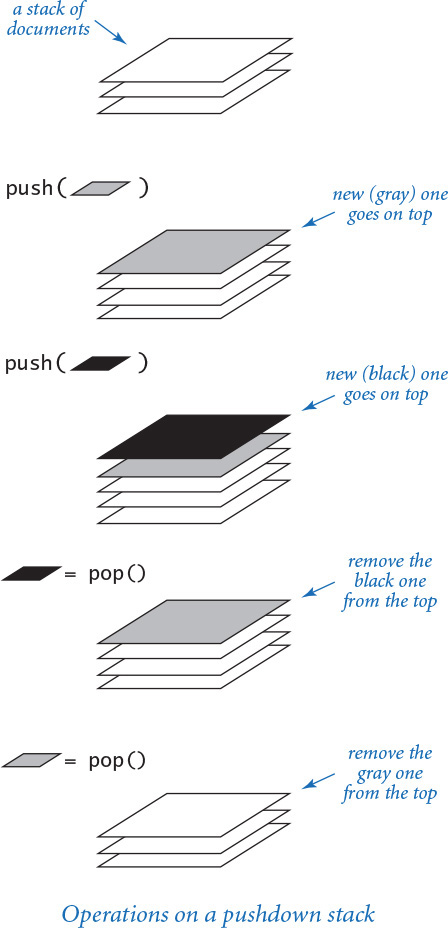
You have likely encountered another common example of a stack when surfing the web. When you click a link, your browser displays the new page (and inserts it onto a stack). You can keep clicking on links to visit new pages, but you can always revisit the previous page by clicking the back button (remove it from a stack). The last-in-first-out policy offered by a stack provides just the behavior that you expect.
Such uses of stacks are intuitive, but perhaps not persuasive. In fact, the importance of stacks in computing is fundamental and profound, but we defer further discussions of applications to later in this section. For the moment, our goal is to make sure that you understand how stacks work and how to implement them.
Programmers have been using stacks since the earliest days of computing. By tradition, we name the stack insert operation push and the stack remove operation pop, as indicated in the API at the top of the next page:

The API includes the core push() and pop() methods, along with a method isEmpty() to test whether the stack is empty and the built-in function len() to get the number of items on the stack. The pop() method raises a run-time error if it is called when the stack is empty. It is the client’s responsibility to call isEmpty() to avoid doing so. Next we consider two implementations of this API: arraystack.py and linkedstack.py.
Important note: When we include performance specifications in an API, as we have in Stack, we consider them to be requirements. An implementation that does not meet them might implement a SlowStack or a SpaceWastingStack, but not a Stack. We want clients to be able to depend on the performance guarantees.
Python list (resizing array) implementation of a stack
Representing a stack with a Python list is a natural idea, but before reading further, it is worthwhile for you to think for a moment about how you would do so.
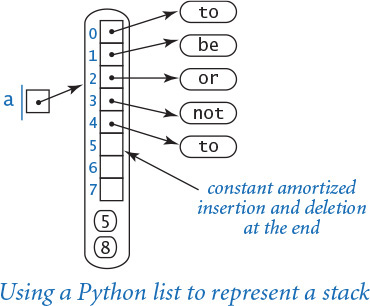
Naturally, you need an instance variable a[] to hold the stack items in a Python list. Should you maintain the items in order of their insertion, with the least recently inserted item in a[0], the second in a[1], and so forth? Or should you maintain the items in reverse order of their insertion? For efficiency, we store the items in order of their insertion because inserting and deleting from the end of a Python list takes constant amortized time per operation (whereas inserting and deleting from the front takes linear time per operation).
We could hardly hope for a simpler implementation of the stack API than stack.py (PROGRAM 4.3.1)—all of the methods are one-liners! The instance variable is a Python list _a[] that holds the items in the stack in order of their insertion. To push an item, we append it to the end of the list using the += operator; to pop an item, we call the pop() method, which removes and returns the item from the end of the list; to determine the size of the stack, we call the built-in len() function. These operations preserve the following properties:
• That stack contains len(_a) items.
• The stack is empty when len(_a) is 0.
• The list _a[] contains the stack items, in order of their insertion.
• The item most recently inserted onto the stack (if nonempty) is _a[len(_a) - 1].
As usual, thinking in terms of invariants of this sort is the easiest way to verify that an implementation operates as intended.
Be sure that you fully understand this implementation. Perhaps the best way to do so is to carefully examine a trace of the list contents for a sequence of push() and pop() operations. The test client in stack.py allows for testing with an arbitrary sequence of operations: it does a push() for each string on standard input except the string consisting of a minus sign, for which it does a pop(). The diagram at right is a trace for the test input shown.
The primary characteristics of this implementation are that it uses space linear in the number of items in the stack and that the push and pop operations take constant amortized time. These properties follow immediately from the corresponding properties for Python lists that we discussed at the end of SECTION 3.1, which, in turn, depend on Python’s resizing array implementation of Python lists. If your programming language provides fixed-size arrays as a built-in data type (but not resizing arrays), you can implement a stack by implementing your own resizing array (see EXERCISE 4.3.45).
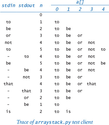
Program 4.3.1 Stack (resizing array) (arraystack.py)
import sys
import stdio
class Stack:
def __init__(self):
self._a = []
def isEmpty(self):
return len(self._a) == 0
def __len__(self):
return len(self._a)
def push(self, item):
self._a += [item]
def pop(self):
return self._a.pop()
def main():
stack = Stack()
while not stdio.isEmpty():
item = stdio.readString()
if item != '-': stack.push(item)
else: stdio.write(stack.pop() + ' ')
stdio.writeln()
if __name__ == '__main__': main()
instance variables
_a[] | stack items
This program defines a Stack class implemented as a Python list (which, in turn, is implemented using a resizing array). The test client reads strings from standard input, popping and writing to standard output when an input string is a minus sign and pushing otherwise.
% more tobe.txt
to be or not to - be - - that - - - is
% python arraystack.py < tobe.txt
to be not that or be
Linked-list implementation of a stack
Next, we consider a completely different way to implement a stack, using a fundamental data structure known as a linked list. Reuse of the word “list” here is a bit confusing, but we have no choice—linked lists have been around much longer than Python.
A linked list is a recursive data structure defined as follows: it is either empty (null) or a reference to a node having a reference to a linked list. The node in this definition is an abstract entity that might hold any kind of data, in addition to the node reference that characterizes its role in building linked lists. As with a recursive program, the concept of a recursive data structure can be a bit mind bending at first, but is of great value because of its simplicity.
With object-oriented programming, implementing linked lists is not difficult. We start with a class for the node abstraction:
class Node:
def __init__(self, item, next):
self.item = item
self.next = next
An object of type Node has two instance variables: item (a reference to an item) and next (a reference to another Node object). The next instance variable characterizes the linked nature of the data structure. To emphasize that we are just using the Node class to structure the data, we define no methods other than the constructor. We also omit leading underscores from the names of the instance variables, thus indicating that it is permissible for code external to the data type (but still within our Stack implementation) to access those instance variables.
Now, from the recursive definition, we can represent a linked list with a reference to a Node object, which contains a reference to an item and a reference to another Node object, which contains a reference to an item and a reference to another Node object, and so forth. The final Node object in the linked list must indicate that it is, indeed, the final Node object. In Python, we accomplish that by assigning None to the next instance variable of the final Node object. Recall that None is a Python keyword—a variable assigned the value None references no object.
Note that our definition of the Node class conforms to our recursive definition of a linked list. With our Node class we can represent a linked list as a variable whose value is either (1) None or (2) a reference to a Node object whose next field is a reference to a linked list. We create an object of type Node by calling the constructor with two arguments: a reference to an item and a reference to the next Node object in the linked list.
For example, to build a linked list that contains the items 'to', 'be', and 'or', we execute this code:
third = Node('or', None)
second = Node('be', third)
first = Node('to', second)
The end result of these operations is actually to create three linked lists:
• third is a linked list—it is a reference to a Node object that contains 'or' and None, which is the reference to an empty linked list.
• second is a linked list—it is a reference to a Node object that contains 'be' and a reference to third, which is a linked list.
• first is a linked list—it is a reference to a Node object that contains 'to' and a reference to second, which is a linked list.
A linked list represents a sequence of items. In this example, first represents the sequence 'to', 'be', 'or'.
We might also use an ordinary array (or Python list) to represent a sequence. For example, we could use the array ['to', 'be', 'or'] to represent the same sequence of strings. One key difference is that linked lists enable efficient insertion of items into (or deletion of items from) either the front or back of the sequence. Next, we consider code to accomplish these tasks.
When tracing code that uses linked lists and other linked structures, we use a visual representation where:
• We draw a rectangle to represent each object.
• We put the values of instance variables within the rectangle.
• We use arrows that point to the referenced objects to depict references.
This visual representation captures the essential characteristic of linked lists. For economy, we use the term link to refer to a Node reference. For simplicity, when the item is a string (as in our examples), we put it within the node rectangle (rather than using the more accurate rendition in which the node holds a reference to a string object, which is external to the node). This visual representation allows us to focus on the links.
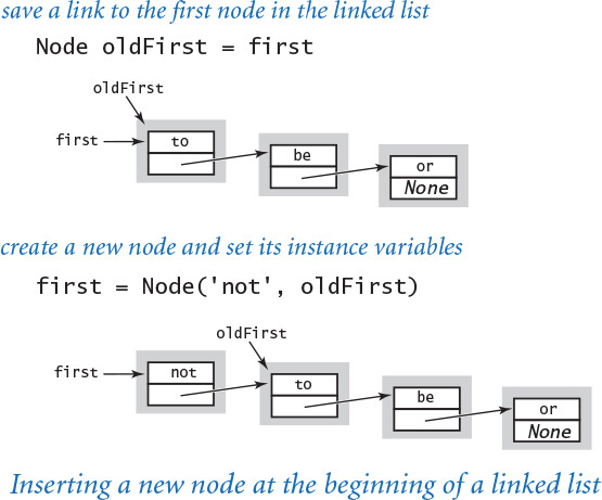
Suppose that you want to remove the first node from a linked list. This operation is easy: simply assign to first the value first.next. Normally, you would retrieve the item (by assigning it to some variable) before doing this assignment, because once you change the variable first, you may lose any access to the node to which it was referring previously. Typically, the Node object becomes an orphan, and Python’s memory management system eventually reclaims it.

Now, suppose that you want to insert a new node into a linked list. The easiest place to do so is at the beginning of the linked list. For example, to insert the string 'not' at the beginning of a given linked list whose first node is first, we save first in a variable oldFirst; create a new Node whose item instance variable is 'not' and whose next instance variable is oldFirst; and assign first to refer to that new Node.
This code for inserting and removing a node from the beginning of a linked list involves just a few assignment statements and thus takes constant time (independent of the length of the list). If you hold a reference to a node at an arbitrary position in a list, you can use similar (but more complicated) code to remove the node after it or to insert a node after it, also in constant time, no matter how long the list. We leave those implementations as exercises (see EXERCISES 4.3.22 and 4.3.24) because inserting and removing at the beginning are the only linked-list operations that we need to implement stacks.

Program 4.3.2 Stack (linked list) (linkedstack.py)
import stdio
class Stack:
def __init__(self):
self._first = None
def isEmpty(self):
return self._first is None
def push(self, item):
self._first = _Node(item, self._first)
def pop(self):
item = self._first.item
self._first = self._first.next
return item
class _Node:
def __init__(self, item, next):
self.item = item
self.next = next
def main():
stack = Stack()
while not stdio.isEmpty():
item = stdio.readString()
if item != '-': stack.push(item)
else: stdio.write(stack.pop() + ' ')
stdio.writeln()
if __name__ == '__main__': main()
instance variable for Stack
_first | first node on list
instance variables for Node
item | list item
next | next node on list
This program defines a Stack class implemented as a linked list, using a private class _Node as the basis for representing the stack as a linked list of _Node objects. The instance variable first refers to the most recently inserted _Node in the linked list. The instance variable next in each _Node refers to the next _Node (the value of next in the final node is None). The test client is the same as in arraystack.py. We defer the __len__() method to EXERCISE 4.3.4.
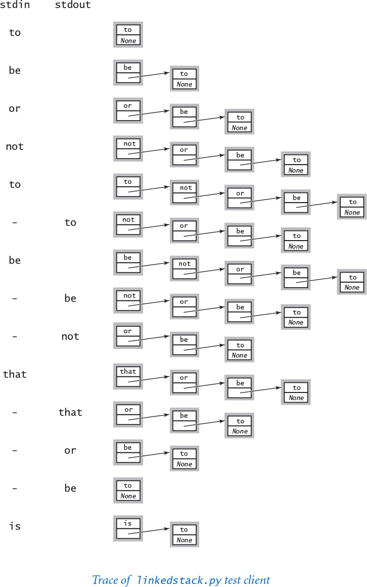
Implementing stacks with linked lists
PROGRAM 4.3.2 (linkedstack.py) uses a linked list to implement a stack, using little more code than the elementary solution that uses a Python list. The implementation is based on a private _Node class that is identical to the Node class that we have been using. Python allows us to define more than one class in a module and use it in this natural way. We make the class private because clients of the Stack data type do not need to know any of the details of the linked lists. As usual, we give the class a name that begins with a leading underscore (that is, we name it _Node instead of Node) to emphasize to Stack clients that they should not access the _Node class directly.
The Stack class defined in linkedstack.py itself has just one instance variable: a reference to the linked list that represents the stack, with the item most recently inserted in the first node. That single link suffices to directly access the item at the top of the stack and also provides access to the rest of the items in the stack for push() and pop().
Again, be sure that you understand this implementation—it is the prototype for several implementations using linked structures that we will examine later in this chapter.
Linked list traversal
While we do not do so in linkedstack.py, many linked-list applications need to iterate over the items in a linked list. To do so, we first initialize a loop index variable x that references the first Node of the linked list. Next, we get the item associated with x by accessing x.item, and then update x to refer to the next Node in the linked list, assigning to it the value of x.next and repeating this process until x is None (which indicates that we have reached the end of the linked list). This process is known as traversing the list.
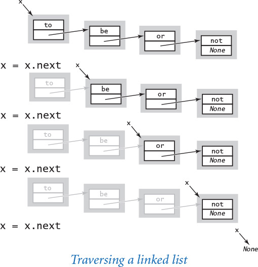
With a linked-list implementation we can implement collections of all sorts without having to worry much about space usage, so linked lists are widely used in programming. Indeed, typical implementations of the Python memory management system are based on maintaining linked lists corresponding to blocks of memory of various sizes. Before the widespread use of high-level languages like Python, the details of memory management and programming with linked lists were critical parts of any programmer’s arsenal. In modern systems, most of these details are encapsulated in the implementations of a few data types like the pushdown stack, including the queue, the symbol table, and the set, which we will consider later in this chapter. If you take a course in algorithms and data structures, you will learn several others and gain expertise in creating and debugging programs that manipulate linked lists. Otherwise, you can focus your attention on understanding the role played by linked lists in implementing these fundamental data types.
For stacks, linked lists are significant because they allow us to implement the push() and pop() methods in constant time in the worst case, while using only a small constant factor of extra space (for the links). If you are uncertain about the value of linked structures, you might think about how you might achieve the same performance specifications for our stack API without using them.
Specifically, arraystack.py does not implement performance specifications in the API, because resizing arrays do not provide a constant-time guarantee for every operation. In many practical situations, the distinction between amortized and guaranteed worst-case performance is a minor one, but you might want to think about whether there might be some huge Python list being resized the next time your phone does not respond to a swipe, the next time your plane is readying for takeoff, or the next time you step on the brakes in your car.
Still, Python programmers usually prefer Python lists (resizing arrays), primarily because of the substantial Python overhead for user-defined types like our linked-list Node. The same principles apply to collections of any sort. For some data types that are more complicated than stacks, resizing arrays are also preferred over linked lists because the ability to access any item in the array in constant time (through indexing) is critical for implementing certain operations (see, for example, RandomQueue in EXERCISE 4.3.40). For some other data types, linked structures are easier to manipulate, as we will see in SECTION 4.4.
Stack applications
Pushdown stacks play an essential role in computation. If you study operating systems, programming languages, and other advanced topics in computer science, you will learn that not only are stacks used explicitly in many applications, but they also serve as the basis for executing programs composed in high-level languages such as Python.

Arithmetic expressions
Some of the first programs that we considered in CHAPTER 1 involved computing the value of arithmetic expressions like this one:
( 1 + ( ( 2 + 3 ) * ( 4 * 5 ) ) )
If you multiply 4 by 5, add 3 to 2, multiply the result, and then add 1, you get the value 101. But how does Python do this calculation? Without going into the details of how Python is built, we can address the essential ideas just by composing a Python program that can take a string as input (the expression) and produce the number represented by the expression as output. For simplicity, we begin with the following explicit recursive definition: an arithmetic expression is either a number or a left parenthesis followed by an arithmetic expression followed by an operator followed by another arithmetic expression followed by a right parenthesis. For simplicity, this definition applies to fully parenthesized arithmetic expressions, which specifies precisely which operators apply to which operands. With a bit more work, we could also handle expressions like 1 + 2 * 3, which use precedence rules instead of parentheses, but we avoid that complication here. For specificity, we support the familiar binary operators *, +, and -, as well as a square-root operator sqrt that takes only one argument. We could easily allow more operators and more kinds of operators to embrace a large class of familiar mathematical expressions, involving trigonometric, exponential, and logarithmic functions and whatever other operators we might wish to include. Our focus here, however, is on understanding how to interpret the string of parentheses, operators, and numbers to enable performing in the proper order the low-level arithmetic operations that are available on any computer.
Arithmetic expression evaluation
Precisely how can we convert an arithmetic expression—a string of characters—to the value that it represents? A remarkably simple algorithm that was developed by Edsgar Dijkstra in the 1960s uses two pushdown stacks (one for operands and one for operators) to do this job. An expression consists of parentheses, operators, and operands (numbers). Proceeding from left to right and taking these entities one at a time, we manipulate the stacks according to four possible cases, as follows:
• Push operands onto the operand stack.
• Push operators onto the operator stack.
• Ignore left parentheses.
• On encountering a right parenthesis, pop an operator, pop the requisite number of operands, and push onto the operand stack the result of applying that operator to those operands.
After the final right parenthesis has been processed, there is one value on the stack, which is the value of the expression. This method may seem mysterious at first, but it is easy to convince yourself that it computes the proper value: anytime the algorithm encounters a subexpression consisting of two operands separated by an operator, all surrounded by parentheses, it leaves the result of performing that operation on those operands on the operand stack. The result is the same as if that value had appeared in the input instead of the subexpression, so we can think of replacing the subexpression by the value to get an expression that would yield the same result. We can apply this argument again and again until we get a single value. For example, the algorithm computes the same value of all of these expressions:
( 1 + ( ( 2 + 3 ) * ( 4 * 5 ) ) )
( 1 + ( 5 * ( 4 * 5 ) ) )
( 1 + ( 5 * 20 ) )
( 1 + 100 )
101
PROGRAM 4.3.3 (evaluate.py) is an implementation of this algorithm. This code is a simple example of an interpreter: a program that interprets the computation specified by a given string and performs the computation to arrive at the result. A compiler is a program that converts the string into code on a lower-level machine that can do the job. This conversion is a more complicated process than the step-by-step conversion used by an interpreter, but it is based on the same underlying mechanism. Initially, Python was based on using an interpreter. Now, however, it includes a compiler that converts arithmetic expressions (and, more generally, Python programs) into code for the Python virtual machine, an imaginary machine that is easy to simulate on an actual computer.
Stack-based programming languages
Remarkably, Dijkstra’s two-stack algorithm also computes the same value as in our example for this expression:
( 1 ( ( 2 3 + ) ( 4 5 * ) * ) + )
In other words, we can put each operator after its two operands instead of between them. In such an expression, each right parenthesis immediately follows an operator so we can ignore both kinds of parentheses, writing the expressions as follows:
1 2 3 + 4 5 * * +
This notation is known as reverse Polish notation, or postfix. To evaluate a postfix expression, we use one stack (see EXERCISE 4.3.13). Proceeding from left to right, taking these entities one at a time, we manipulate the stacks according to just two possible cases:
• Push operands onto the operand stack.
• On encountering an operator, pop the requisite number of operands and push onto the operand stack the result of applying the operator to those operands.

Again, this process leaves one value on the stack, which is the value of the expression. This representation is so simple that some programming languages, such as Forth (a scientific programming language) and PostScript (a page description language that is used on most printers) use explicit stacks. For example, the string 1 2 3 + 4 5 * * + is a legal program in both Forth and PostScript that leaves the value 101 on the execution stack. Aficionados of these and similar stack-based programming languages prefer them because they are simpler for many types of computation. Indeed, the Python virtual machine itself is stack-based.
Program 4.3.3 Expression evaluation (evaluate.py)
import stdio
import math
from arraystack import Stack
ops = Stack()
values = Stack()
while not stdio.isEmpty():
token = stdio.readString()
if token == '+': ops.push(token)
elif token == '-': ops.push(token)
elif token == '*': ops.push(token)
elif token == 'sqrt': ops.push(token)
elif token == ')':
op = ops.pop()
value = values.pop()
if op == '+': value = values.pop() + value
elif op == '-': value = values.pop() - value
elif op == '*': value = values.pop() * value
elif op == 'sqrt': value = math.sqrt(value)
values.push(value)
elif token != '(':
values.push(float(token))
stdio.writeln(values.pop())
ops | operator stack
values | operand stack
token | current token
value | current value
This Stack client reads a fully parenthesized numeric expression from standard input, uses Dijkstra’s two-stack algorithm to evaluate it, and writes the resulting number to standard output. It illustrates an essential computational process: interpreting a string as a program and executing that program to compute the desired result. Executing a Python program is nothing other than a more complicated version of this same process.

Function-call abstraction
You may have noticed a pattern in the formal traces that we have shown throughout this book. When the flow of control enters a function, Python creates the function’s parameter variables on top of the other variables that might already exist. As the function executes, Python creates the function’s local variables—again on top of the other variables that might already exist. When flow of control returns from a function, Python destroys that function’s local and parameter variables. In that sense Python creates and destroys parameter and local variables in stack-like fashion: the variables that were created most recently are the first to be destroyed.
Indeed, most programs use stacks implicitly because they support a natural way to implement function calls, as follows: at any point during the execution of a function, define its state to be the values of all of its variables and a pointer to the next instruction to be executed. One of the fundamental characteristics of computing environments is that every computation is fully determined by its state (and the value of its inputs). In particular, the system can suspend a computation by saving away its state, then restart it by restoring the state. If you take a course about operating systems, you will learn the details of this process, because it is critical to much of the behavior of computers that we take for granted (for example, switching from one application to another is simply a matter of saving and restoring state). Now, the natural way to implement the function-call abstraction, which is used by almost all modern programming environments, is to use a stack. To call a function, push the state on a stack. To return from a function call, pop the state from the stack to restore all variables to their values before the function call, substitute the function return value (if there is one) in the expression containing the function call (if there is one), and resume execution at the next instruction to be executed (whose location was saved as part of the state of the computation). This mechanism works whenever functions call one another, even recursively. Indeed, if you think about the process carefully, you will see that it is essentially the same process that we just examined in detail for expression evaluation. A program is a sophisticated expression.
The pushdown stack is a fundamental computational abstraction. Stacks have been used for expression evaluation, implementing the function-call abstraction, and other basic tasks since the earliest days of computing. We will examine another (tree traversal) in SECTION 4.4. Stacks are used explicitly and extensively in many areas of computer science, including algorithm design, operating systems, compilers, and numerous other computational applications.
FIFO queues
A FIFO queue (or just a queue) is a collection that is based on the first-in first-out (FIFO) policy.
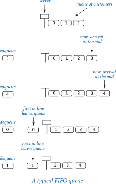
The policy of doing tasks in the same order that they arrive is one that we encounter frequently in everyday life, from people waiting in line at a theater, to cars waiting in line at a toll booth, to tasks waiting to be serviced by an application on your computer.
One bedrock principle of any service policy is the perception of fairness. The first idea that comes to mind when most people think about fairness is that whoever has been waiting the longest should be served first. That is precisely the FIFO discipline, so queues play a central role in numerous applications. Queues are a natural model for so many everyday phenomena—their properties were studied in detail even before the advent of computers.
As usual, we begin by articulating an API. Again by tradition, we name the queue insert operation enqueue and the remove operation dequeue, as indicated in the API below.

Applying our knowledge from stacks, we can use either Python lists (resizing arrays) or linked lists to develop implementations where the operations take constant time and the memory associated with the queue grows and shrinks with the number of elements in the queue. As with stacks, each of these implementations represents a classic programming exercise. You may wish to think about how you might achieve these goals in an implementation before reading further.
Linked-list implementation
To implement a queue with a linked list, we keep the items in order of their arrival (the reverse of the order that we used in linkedstack.py). The implementation of dequeue() is the same as the pop() implementation in linkedstack.py (save the item in the first node, remove the first node from the queue, and return the saved item). Implementing enqueue(), however, is a bit more challenging: how do we add a node to the end of a linked list? To do so, we need a link to the last node in the list, because that node’s link has to be changed to reference a new node containing the item to be inserted. In Stack, the only instance variable is a reference to the first node in the linked list; with just that information available, our only recourse is to traverse all the nodes in the linked list to get to the end. That solution is unattractive when lists might be lengthy. A reasonable alternative is to maintain a second instance variable that always references the last node in the linked list. Adding an extra instance variable that needs to be maintained is not something that should be taken lightly, particularly in linked-list code, because every method that modifies the linked list needs code to check whether that variable needs to be modified (and to make the necessary modifications). For example, removing the first node in the linked list might involve changing the reference to the last node in the linked list, since when there is only one node in the linked list, it is both the first one and the last one! Similarly, we need an extra check when adding a new node to an empty linked list. Details like these make linked-list code notoriously difficult to debug.
Program 4.3.4 FIFO queue (linked list) (linkedqueue.py)
class Queue:
def __init__(self):
self._first = None
self._last = None
self._n = 0
def isEmpty(self):
return self._first is None
def enqueue(self, item):
oldLast = self._last
self._last = _Node(item, None)
if self.isEmpty(): self._first = self._last
else: oldLast.next = self._last
self._n += 1
def dequeue(self):
item = self._first.item
self._first = self._first.next
if self.isEmpty(): self._last = None
self._n -= 1
return item
def __len__(self):
return self._n
class _Node:
def __init__(self, item, next):
self.item = item
self.next = next
instance variables for Queue
_first | first node on list
_last | last node on list
_n | number of items
instance variables for Node
item | list item
next | next node on list
This program defines a Queue class implemented as a linked list. The implementation is very similar to our linked-list stack implementation (PROGRAM 4.3.2): dequeue() is almost the same as pop(), but enqueue() links the new item onto the end of the list, not the beginning as in push(). To do so, it maintains an instance variable that references the last node on the list. The test client is similar to the ones we have been using (it reads strings from standard input, dequeuing and writing to standard output when an input string is a minus sign, enqueuing the string otherwise) and is omitted.

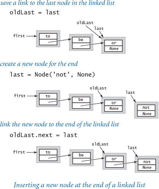
PROGRAM 4.3.4 (linkedqueue.py) is a linked-list implementation of Queue that has the same performance properties as Stack: all of the methods are constant-time operations, and space usage is linear in the number of items on the queue.
Resizing array implementation
It is also possible to develop a FIFO queue implementation that is based on an explicit resizing array representation that has the same performance characteristics as those that we developed for a stack in arraystack.py (PROGRAM 4.3.1). This implementation is a worthy and classic programming exercise that you are encouraged to pursue further (see EXERCISE 4.3.46). It might be tempting to use one-line calls on Python list methods, as in PROGRAM 4.3.1. However, the methods for inserting or deleting items at the front of a Python list will not fill the bill, as they take linear time (see EXERCISES 4.3.16 and 4.3.17). For example, if a is a list with n items, then operations such as a.pop(0) and a.insert(0, item) take time proportional to n (and not constant amortized time). Again, an implementation that does not provide the specified performance guarantees might implement a SlowQueue, but not a Queue.
Random queues
Even though they are widely applicable, there is nothing sacred about the FIFO and LIFO disciplines. It makes perfect sense to consider other rules for removing items. One of the most important to consider is a data type for which dequeue() removes a random item (sampling without replacement) and sample() returns a random item without removing it from the queue (sampling with replacement). Such actions are precisely called for in numerous applications, some of which we have already considered, starting with sample.py (PROGRAM 1.4.1). With a Python list (resizing array) representation, implementing sample() is straightforward, and we can use the same idea as in PROGRAM 1.4.1 to implement dequeue() (exchange a random item with the last item before removing it). We use the name RandomQueue to refer to this data type (see EXERCISE 4.3.40). Note that this solution depends on using a resizing-array representation (Python list): it is not possible to access a random item in a linked list in constant time because we have to start from the beginning of the list and traverse links one at a time to access it. With a Python list (resizing array), all of the operations take constant amortized time.
The stack, queue, and random queue APIs are essentially identical—they differ only in the choice of class and method names (which are chosen arbitrarily). Thinking about this situation is a good way to cement your understanding of the basic issues surrounding data types that we introduced in SECTION 3.3. The true differences among these data types are in the semantics of the remove operation—which item is to be removed? The differences between stacks and queues are embodied in the English-language descriptions of what they do. These differences are akin to the differences between math.sin(x) and math.log(x), but we might want to articulate them with a formal description of stacks and queues (in the same way as we have mathematical descriptions of the sine and logarithm functions). But precisely describing what we mean by first-in-first-out or last-in-first-out or random-out is not so simple. For starters, which language would you use for such a description? English? Python? Mathematical logic? The problem of describing how a program behaves is known as the specification problem, and it leads immediately to deep issues in computer science. One reason for our emphasis on clear and concise code is that the code itself can serve as the specification for simple data types such as stacks and queues.
Queue applications
In the past century, FIFO queues proved to be accurate and useful models in a broad variety of applications, ranging from manufacturing processes to telephone networks to traffic simulations. A field of mathematics known as queuing theory has been used with great success to help understand and control complex systems of all kinds. FIFO queues also play an important role in computing. You often encounter queues when you use your computer: a queue might hold songs on a playlist, documents to be printed, or events in a game.
Perhaps the ultimate queue application is the Internet itself, which is based on huge numbers of messages moving through huge numbers of queues that have all sorts of different properties and are interconnected in all sorts of complicated ways. Understanding and controlling such a complex system involves solid implementations of the queue abstraction, application of mathematical results of queueing theory, and simulation studies involving both. We consider next a classic example to give a flavor of this process.
M/M/1 queue
One of the most important queueing models is known as an M/M/1 queue, which has been shown to accurately model many real-world situations, such as a single line of cars entering a toll booth or patients entering an emergency room. The M stands for Markovian or memoryless and indicates that both arrivals and services are Poisson processes: both the interarrival times and service times obey an exponential distribution (see EXERCISE 2.2.12) and the 1 indicates that there is one server. An M/M/1 queue is parameterized by its arrival rate λ (for example, the number of cars per minute arriving at the toll booth) and its service rate μ (for example, the number of cars per minute that can pass through the toll booth) and is characterized by three properties:
• There is one server—a FIFO queue.
• Interarrival times to a queue obey an exponential distribution with rate λ per minute.
• Service times from a nonempty queue obey an exponential distribution with rate μ per minute.
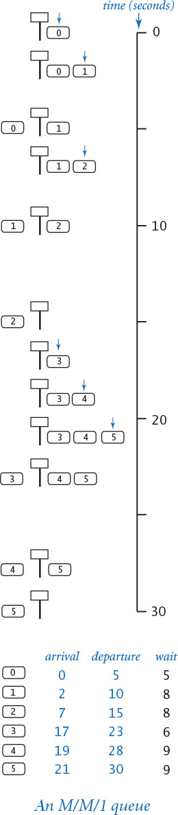
The average time between arrivals is 1/λ minutes and the average time between services (when the queue is nonempty) is 1/μ minutes. So, the queue will grow without bound unless μ > λ; otherwise, customers enter and leave the queue in an interesting dynamic process.
Analysis
In practical applications, people are interested in the effect of the parameters λ and μ on various properties of the queue. If you are a customer, you may want to know the expected amount of time you will spend in the system; if you are designing the system, you might want to know how many customers are likely to be in the system, or something more complicated, such as the likelihood that the queue size will exceed a given maximum size. For simple models, probability theory yields formulas expressing these quantities as functions of λ and μ. For M/M/1 queues, it is known that:
• The average number of customers in the system L is λ / (μ – λ).
• The average time a customer spends in the system W is 1 / (μ – λ).
For example, if the cars arrive at a rate of λ = 10 per minute and the service rate is μ = 15 per minute, then the average number of cars in the system will be 2 and the average time that a customer spends in the system will be 1/5 minutes or 12 seconds. These formulas confirm that the wait time (and queue length) grows without bound as λ approaches μ. They also obey a general rule known as Little’s law: the average number of customers in the system is λ times the average time a customer spends in the system (L = λW) for many types of queues.
Simulation
PROGRAM 4.3.5 (mm1queue.py) is a Queue client that you can use to validate these sorts of mathematical results. It is a simple example of an event-based simulation: we generate events that take place at particular times and adjust our data structures accordingly for the events, simulating what happens at the time they occur. In an M/M/1 queue, there are two kinds of events: we either have a customer arrival or a customer service. In turn, we maintain two variables:
• nextService is the time of the next service.
• nextArrival is the time of the next arrival.
To simulate an arrival event, we enqueue a float nextArrival (the time of arrival); to simulate a service, we dequeue a float, compute the wait time wait (which is the time that the service is completed minus the time that the customer arrived and entered the queue), and add the wait time to a histogram (see PROGRAM 3.2.3). The shape that results after a large number of trials is characteristic of the M/M/1 queueing system. From a practical point of view, one of the most important characteristics of the process, which you can discover for yourself by running mm1queue.py for various values of the parameters λ and μ, is that the average time a customer spends in the system (and the average number of customers in the system) can increase dramatically when the service rate approaches the arrival rate. When the service rate is high, the histogram has a visible tail where the frequency of customers having a given wait time decreases to a negligible duration as the wait time increases. But when the service rate is close to the arrival rate, the tail of the histogram stretches to the point that most values are in the tail, so the frequency of customers having at least the highest wait time displayed dominates.
Program 4.3.5 M/M/1 queue simulation (mm1queue.py)
import sys
import stddraw
import stdrandom
from linkedqueue import Queue
from histogram import Histogram
lambd = float(sys.argv[1])
mu = float(sys.argv[2])
histogram = Histogram(60 + 1)
queue = Queue()
stddraw.setCanvasSize(700, 500)
nextArrival = stdrandom.exp(lambd)
nextService = nextArrival + stdrandom.exp(mu)
while True:
while nextArrival < nextService:
queue.enqueue(nextArrival)
nextArrival += stdrandom.exp(lambd)
arrival = queue.dequeue()
wait = nextService - arrival
stddraw.clear()
histogram.addDataPoint(min(60, int(round(wait))))
histogram.draw()
stddraw.show(20.0)
if queue.isEmpty():
nextService = nextArrival + stdrandom.exp(mu)
else:
nextService = nextService + stdrandom.exp(mu)
lambd | arrival rate λ
mu | service rate μ
histogram | histogram
queue | M/M/1 queue
nextArrival | time of next arrival
nextService | time of next service completion
arrival | arrival time of next customer to be serviced
wait | time on queue
This program accepts float command-line arguments lambd and mu and simulates an M/M/1 queue with arrival rate lambd and service rate mu, producing a dynamic Histogram of the wait times. Time is tracked with two variables nextArrival and nextService and a single Queue of floats. The value of each item on the queue is the (simulated) time it entered the queue. Example plots produced by the program are shown and discussed on the next page.
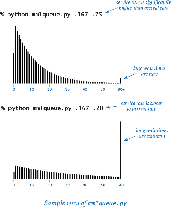
As in many other applications that we have studied, the use of simulation to validate a well-understood mathematical model is a starting point for studying more complex situations. In practical applications of queues, we may have multiple queues, multiple servers, multistage servers, limits on queue length, and many other restrictions. Moreover, the distributions of interarrival and service times may not be possible to characterize mathematically. In such situations, we may have no recourse but to use simulations. It is quite common for a system designer to build a computational model of a queuing system (such as mm1queue.py) and to use it to adjust design parameters (such as the service rate) to properly respond to the outside environment (such as the arrival rate).
Resource allocation
Next, we examine another application that illustrates the data structures that we have been considering. A resource-sharing system involves a large number of loosely cooperating servers that want to share resources. Each server agrees to maintain a queue of items for sharing, and a central authority distributes the items to the servers (and informs users where they may be found). For example, the items might be songs, photos, or videos to be shared by a large number of users. To fix ideas, we will think in terms of millions of items and thousands of servers.
We will consider the kind of program that the central authority might use to distribute the items, ignoring the dynamics of deleting items from the systems, adding and deleting servers, and so forth.
If we use a round-robin policy, cycling through the servers to make the assignments, we get a balanced allocation, but it is rarely possible for a distributor to have such complete control over the situation. For example, there might be a large number of independent distributors, so none of them could have up-to-date information about the servers. Accordingly, such systems often use a random policy, where the assignments are based on random choice. An even better policy is to choose a random sample of servers and assign a new item to the one that has smallest number of items. For small queues, differences among these policies is immaterial, but in a system with millions of items on thousands of servers, the differences can be quite significant, since each server has a fixed amount of resources to devote to this process. Indeed, similar systems are used in Internet hardware, where some queues might be implemented in special-purpose hardware, so queue length translates directly to extra equipment cost. But how big a sample should we take?
PROGRAM 4.3.6 (loadbalance.py) is a simulation of the sampling policy, which we can use to study this question. This program makes good use of the RandomQueue data type that we have been considering to provide an easily understood program that we can use for experimentation. The simulation maintains a random queue of queues and builds the computation around an inner loop where each new request for service goes on the smallest of a sample of queues, using the sample() method from RandomQueue to randomly sample queues. The surprising end result is that samples of size 2 lead to near-perfect balancing, so there is no point in taking larger samples.
Program 4.3.6 Load-balancing simulation (loadbalance.py)
import sys
import stddraw
import stdstats
from linkedqueue import Queue
from randomqueue import RandomQueue
m = int(sys.argv[1])
n = int(sys.argv[2])
t = int(sys.argv[3])
servers = RandomQueue()
for i in range(m):
servers.enqueue(Queue())
for j in range(n):
best = servers.sample()
for k in range(1, t):
queue = servers.sample()
if len(queue) < len(best):
best = queue
best.enqueue(j)
lengths = []
while not servers.isEmpty():
lengths += [len(servers.dequeue())]
stddraw.setYscale(0, 2.0*n/m)
stdstats.plotBars(lengths)
stddraw.show()
m | number of servers
n | number of items
t | sample size
servers | queues
best | shortest in sample
lengths | queue lengths
This Queue and RandomQueue client simulates the process of assigning n items to a set of m servers. Requests are put on the shortest of a sample of t queues chosen at random.
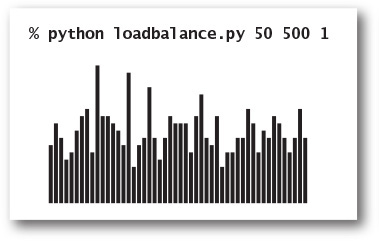
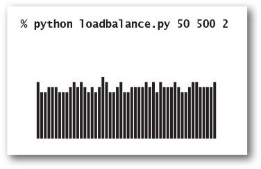
We have considered in detail the issues surrounding the time and memory usage of basic implementations of the stack and queue APIs not just because these data types are important and useful, but also because you are likely to encounter the very same issues in the context of your own data-type implementations.
Should you use a pushdown stack, a FIFO queue, or a random queue when developing a client that maintains collections of data? The answer to this question depends on a high-level analysis of the client to determine which of the LIFO, FIFO, or random disciplines is appropriate.
Should you use a linked list or a resizing array to structure your data? The answer to this question depends on low-level analysis of performance characteristics. A linked list has the advantage that you can add items at either end but the disadvantage that you cannot access an arbitrary item in constant time. A resizing array has the advantage that you can access any item in constant time but the disadvantage that the constant running time is only for insertions and deletions at one end (and it is constant time only in the amortized sense). Each data structure is appropriate in various different situations; you are likely to encounter both in most programming environments.
The careful attention to performance guarantees that we have emphasized in our Stack and Queue APIs are not to be taken for granted. They are just the first in a progression of data types that provide the underpinnings of our computational infrastructure. The next section is devoted to an even more important one, the symbol table, and you will learn about others when you take a course on data structures and algorithms. By now, you know that learning to use a new data type is not so different from learning to ride a bicycle or implement helloworld.py: it seems completely mysterious until you have done it for the first time, but quickly becomes second nature. And learning to design and implement a new data type by developing a new data structure is a challenging, fruitful, and satisfying activity. As you will see in the exercises that follow, stacks, queues, linked lists, and resizing arrays raise a host of fascinating questions, but they are also just the beginning.