Chapter Three. Object-Oriented Programming
Your next step to programming effectively is conceptually simple. Now that you know how to use built-in data types, you will learn in this chapter how to use, create, and design higher-level data types.
An abstraction is a simplified description of something that captures its essential elements while suppressing all other details. In science, engineering, and programming, we are always striving to understand complex systems through abstraction. In Python programming, we do so with object-oriented programming, where we break a large and potentially complex program into a set of interacting elements, or objects. The idea originates from modeling (in software) real-world entities such as electrons, people, buildings, or solar systems and readily extends to modeling abstract entities such as bits, numbers, colors, images, or programs.
As discussed in SECTION 1.2, a data type is a set of values and a set of operations defined on those values. In Python, the values and operations for many data types such as int and float are predefined. In object-oriented programming, we compose code to create new data types.
This ability to define new data types and to manipulate objects holding data-type values is also known as data abstraction, and leads us to a style of modular programming that naturally extends the function abstraction style that was the basis for CHAPTER 2. A data type allows us to isolate data as well as functions. Our mantra for this chapter is this: Whenever you can clearly separate data and associated tasks within a computation, you should do so.
3.1 Using Data Types
Organizing data for processing is an essential step in the development of a computer program. Programming in Python is largely based on doing so with data types that are designed to support object-oriented programming, a style of programming that integrates code and data.
3.1.1 Identifying a potential gene
3.1.5 Converting color to grayscale
3.1.8 Visualizing electric potential
3.1.10 Screen scraping for stock quotes
Programs in this section
You certainly noticed in the first two chapters of this book that our programs were confined to operations on numbers, booleans, and strings. Of course, the reason is that the Python data types that we’ve encountered so far—int, float, bool, and str—manipulate numbers, booleans, and strings, using familiar operations. In this chapter, we begin to consider other data types.
We first examine a host of new operations on objects of type str, which will introduce you to object-oriented programming because most of these operations are implemented as methods that manipulate objects. Methods are very similar to functions, except that each method call is explicitly associated with a specified object. To illustrate the natural style of programming induced by the use of methods, we consider a string-processing application from genomics.
Even more significantly, you will learn in SECTION 3.2 to define your own data types to implement any abstraction whatsoever. This ability is crucial in modern programming. No library of modules can meet the needs of all possible applications, so programmers routinely create data types to meet their own needs.
In this section, we focus on client programs that use existing data types, to give you some concrete reference points for understanding these new concepts and to illustrate their broad reach. We introduce constructors to create objects from a data type and methods to operate on their values. We consider programs that manipulate electrical charges, colors, images, files, and web pages—quite a leap from the built-in data types that we used in previous chapters.
Methods
In SECTION 1.2, you learned that a data type is a set of values and a set of operations defined on those values, and you learned details of Python’s built-in data types int, bool, float, and str. You also learned that all data in a Python program are represented by objects and relationships among objects. Since then, we have focused on composing programs that use the operations associated with the built-in types to manipulate objects of those types. To do so, we have used conditionals, loops, and functions, which enable us to build large programs where the flow of control from operation to operation is well understood. In this section, we put these concepts together.
In the programs that we have encountered so far, we apply data-type operations using built-in operators such as +, -, *, /, and []. Now, we are going to introduce a new way to apply data-type operations that is more general. A method is a function associated with a specified object (and, by extension, with the type of that object). That is, a method corresponds to a data-type operation.
We can call (or invoke) a method by using a variable name, followed by the dot operator (.), followed by the method name, followed by a list of arguments delimited by commas and enclosed in parentheses. As a simple example, Python’s built-in int type has a method named bit_length(), so you can determine the number of bits in the binary representation of an int value as follows:
x = 3 ** 100
bits = x.bit_length()
stdio.writeln(bits)
This code writes 159 to standard output, telling you that 3100 (a huge integer) has 159 bits when expressed in binary.
The syntax and behavior of method calls is nearly the same as the syntax and behavior of function calls. For example, a method can take any number of arguments, those arguments are passed by object reference, and the method returns a value to its caller. Similarly, like a function call, a method call is an expression, so you can use it anywhere in your program where you would use an expression. The main difference in syntactic: you invoke a method using a specified object and the dot operator.
In “object-oriented programming,” we usually prefer method-call syntax to function-call syntax because it emphasizes the role of the object. This approach has proved for decades to be a fruitful way to develop programs, particularly those that are developed to build and understand models of the real world.
Distinction between methods and functions
The key difference between a function and a method is that a method is associated with a specified object. You can think of this specified object as an extra argument that gets passed to a function, in addition to the ordinary methods argument. You can distinguish between method calls and function calls in client code by looking to the left of the dot operator: a function call typically uses a module name and a method call typically uses a variable name. These differences are illustrated at left and summarized in the table at the bottom of this page.

String processing
Out of necessity, we have been using the str data type from the beginning of this book, to create human-readable output for our programs. Your experience with using str demonstrates that you do not need to know how a data type is implemented to be able to use it (one of several mantras we repeat in this book because of its importance). You know that str values are sequences of characters and that you can perform the operation of concatenating two str values to produce a str result.
Python’s str data type includes many other operations, as documented in the API on the facing page. It is one of Python’s most important data types because string processing is critical to many computational applications. Strings lie at the heart of our ability to compile and execute Python programs and to perform many other core computations; they are the basis of the information-processing systems that are critical to most business systems; people use them every day when typing into email, blog, or chat applications or preparing documents for publication; and they are critical ingredients in scientific progress in several fields, particularly molecular biology.

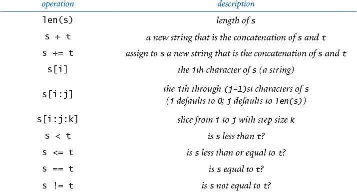

On closer examination, you will see that the operations in the str API can be divided into three categories:
• Built-in operators +, +=, [], [:], in, not in, and the comparison operators, which are characterized by special symbols and syntax
• A built-in function len() with standard function-call syntax
• Methods upper(), startswith(), find(), and so forth, which are distinguished in the API with a variable name followed by the dot operator
From this point forward, any API that we might consider will have these kinds of operations. Next, we consider each of them in turn.

Built-in operators
An operator (or function) that you can apply to more than one type of data is said to be polymorphic. Polymorphism is an important feature of Python programming, and several built-in operators allow you to compose compact code using familiar operators for processing any type of data. You have already been using the + operator, familiar for numbers, for string concatenation. The API tells you that you can use the [] operator, familiar for arrays, to extract a single character from a string and the [:] operator to extract a substring from a string. Not all data types provide implementations for all operators—for example, the operator / is not defined for strings because it makes no sense to divide two strings.
Built-in functions
Python also builds in a number of polymorphic functions, such as the len() function, that are likely to make sense for numerous data types. When a data type implements such a function, Python automatically calls that implementation, based on the type of the argument. Polymorphic functions are like polymorphic operators, but without the special syntax.
Methods
We include built-in operators and built-in functions for convenience (and to conform to Python norms), but most of our effort in creating data types goes into developing methods that operate on object values, such as upper(), startswith(), find(), and the other methods in the str API.
In point of fact, these three kinds of operations end up being the same in implementations, as you will see in SECTION 3.2. Python automatically maps built-in operators and functions to special methods, using the convention that such special methods have double underscores before and after their names. For example, s + t is equivalent to the method call s.__add__(t) and len(s) is equivalent to the method call s.__len__(). We never use the double underscore form in client code, but we do use it to implement special methods, as you will see in SECTION 3.2.
The table below gives several examples of simple string-processing applications that illustrate the utility of the various operations in Python’s str data type. The examples are just an introduction; we examine a more sophisticated client next.

String-processing application: genomics
To give you more experience with string processing, we will give a very brief overview of the field of genomics and consider a program that a bioinformatician might use to identify potential genes. Biologists use a simple model to represent the building blocks of life, in which the letters A, C, T, and G represent the four bases in the DNA of living organisms. In each living organism, these basic building blocks appear in a set of long sequences (one for each chromosome) known as a genome. Understanding properties of the genome is a key to understanding the processes that manifest themselves in living organisms. The genomic sequences for many living things are known, including the human genome, which is a sequence of about 3 billion bases. Since the sequences have been identified, scientists have begun composing computer programs to study their structure. String processing is now one of the most important methodologies—experimental or computational—in molecular biology.
Gene prediction
A gene is a substring of a genome that represents a functional unit of critical importance in understanding life processes. A gene consists of a sequence of codons, each of which is a sequence of three bases that represents one amino acid. The start codon ATG marks the beginning of a gene, and any of the stop codons TAG, TAA, or TGA marks the end of a gene (and no other occurrences of any of these stop codons can appear within the gene). One of the first steps in analyzing a genome is to identify its potential genes, which is a string-processing problem that Python’s str data type equips us to solve.
PROGRAM 3.1.1 (potentialgene.py) is a program that serves as a first step. It takes a DNA sequence as a command-line argument and determines whether it corresponds to a potential gene based on the following criteria: length is a multiple of 3, starts with the start codon, ends with the stop codon, and has no intervening stop codons. To make the determination, the program uses a mixture of string methods, built-in operators, and built-in functions.
Although the rules that define genes are a bit more complicated than those we have sketched here, potentialgene.py exemplifies how a basic knowledge of programming can enable a scientist to study genomic sequences more effectively.
In the present context, our interest in str is that it illustrates what a data type can be—a well-developed encapsulation of an important abstraction that is useful to clients. Python’s language mechanisms, from polymorphic functions and operators to methods that operate on object values, help us achieve that goal. Next, we proceed to numerous other examples.
Program 3.1.1 Identifying a potential gene (potentialgene.py)
import sys
import stdio
def isPotentialGene(dna):
# number of bases is a multiple of 3
if (len(dna) % 3) != 0: return False
# starts with start codon
if not dna.startswith('ATG'): return False
# no intervening stop codons
for i in range(len(dna) - 3):
if i % 3 == 0:
if dna[i:i+3] == 'TAA': return False
if dna[i:i+3] == 'TAG': return False
if dna[i:i+3] == 'TGA': return False
# ends with a stop codon
if dna.endswith('TAA'): return True
if dna.endswith('TAG'): return True
if dna.endswith('TGA'): return True
return False
dna = sys.argv[1]
stdio.writeln(isPotentialGene(dna))
This program takes a DNA sequence as a command-line argument and determines whether it corresponds to a potential gene: length is a multiple of 3, starts with the start codon (ATG), ends with a stop codon (TAA or TAG or TGA), and has no intervening stop codons.
% python potentialgene.py ATGCGCCTGCGTCTGTACTAG
True
% python potentialgene.py ATGCGCTGCGTCTGTACTAG
False
A user-defined data type
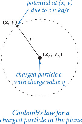
As a running example of a user-defined data type, we will consider a data type Charge for charged particles. In particular, we are interested in a two-dimensional model that uses Coulomb’s law, which tells us that the electric potential at a point due to a given charged particle is represented by V = kq/r, where q is the charge value, r is the distance from the point to the charge, and k =8.99×10⁹ N m2/C2 is a constant known as the electrostatic constant, or Coulomb’s constant. For consistency, we use SI (Système International d’Unités): in this formula, N designates newtons (force), m designates meters (distance), and C represent coulombs (electric charge). When there are multiple charged particles, the electric potential at any point is the sum of the potentials due to each charge. Our interest is computing the potential at various points in the plane due to a given set of charged particles. To do so, we will compose programs that create and manipulate Charge objects.
Application programming interface
To fulfill our mantra promise that you do not need to know how a data type is implemented to use it, we specify the behavior of the Charge data type by listing its operations in an API, deferring the discussion of the implementation until SECTION 3.2.

The first entry in the API, which has the same name as the data type, is known as a constructor. Clients call the constructor to create new objects; each call to the Charge constructor creates exactly one new Charge object. The other two entries define the data-type operations. The first is a method potentialAt(), which computes and returns the potential due to the charge at the given point (x, y). The second is the built-in function str(), which returns a string representation of the charged particle. Next, we discuss how to make use of this data type in client code.
File conventions
The code that defines a user-defined data type resides in a .py file. By convention, we define each data type in a distinct .py file, with the same name as the data type (but not capitalized). Thus, the Charge data type is found in a file named charge.py. To compose a client program that uses the Charge data type, we put the following import statement at the top of the client .py file:
from charge import Charge
Note that the format of the import statement that we use with user-defined data types differs from the format we use with functions. As usual, you must make charge.py available to Python, either by putting it in the same directory as your client code or by using your operating system’s path mechanism (see the Q&A at the end of SECTION 2.2).
Creating objects
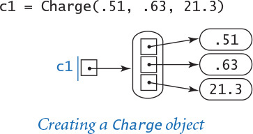
To create an object from a user-defined data type, you call its constructor, which directs Python to create a new individual object. You call a constructor just as if it were a function, using the name of the data type, followed by the constructor’s arguments enclosed in parentheses and separated by commas. For example, Charge(x0, y0, q0) creates a new Charge object with position (x0, y0) and charge value q0 and returns a reference to the new object. Typically, you call a constructor to create a new object and set a variable to reference that object in the same line of code, as in the example shown in the diagram at right. Once you have created the object, the values x0, y0, and q0 belong to the object. As usual, it is helpful to picture the newly created variable and object as in the memory diagram at right.
You can create any number of objects of the same data type. Recall from SECTION 1.2 that each object has its own identity, type, and value. So, while any two objects reside at distinct places in computer memory, they may be of the same type and store the same value. For example, the code in the diagram at the top of the next page creates three distinct Charge objects. The variables c1 and c3 reference distinct objects, even though the two objects store the same value. In other words, the objects referenced by c1 and c3 are equal (that is, they are objects of the same data type and they happen to store the same value), but they are not identical (that is, they have distinct identities because they reside in different places in computer memory). In contrast, c2 and c4 refer to the same object—they are aliases.
Calling a method
As discussed at the beginning of this section, we typically use a variable name to identify the object to be associated with the method we intend to call. For our example, the method call c1.potentialAt(.20, .50) returns a float that represents the potential at the query point (0.20, 0.50) due to the Charge object referenced by c1. The distance between the query point and the charge location is 0.34, so this potential is 8.99 × 109 × 0.51 / 0.34 = 1.35 × 10¹⁰.

String representation
In any data-type implementation, it is typically worthwhile to include an operation that converts an object’s value to a string. Python has a built-in function str() for this purpose, which you been using from the beginning to convert integers and floats to strings for output. Since our Charge API has a str() implementation, any client can call str() to get a string representation of a Charge object. For our example, the call str(c1) returns the string '21.3 at (0.51, 0.63)'. The nature of the conversion is completely up to the implementation, but usually the string encodes the object’s value in a human-readable format. We will examine the exact mechanism behind this convention when we discuss the implementation, in SECTION 3.2.
These mechanisms are summarized in the client chargeclient.py (PROGRAM 3.1.2), which creates two Charge objects and computes the total potential due to the two charges at a query point taken from the command line. This code illustrates the idea of developing an abstract model (for a charged particle) and separating the code that implements the abstraction (which you haven’t even seen yet) from the code that uses it. This is a turning point in this book: we have not yet seen any code of this nature, but virtually all of the code that we compose from this point forward will be based on defining and invoking methods that implement data-type operations.
Program 3.1.2 Charged-particle client (chargeclient.py)
import sys
import stdio
from charge import Charge
x = float(sys.argv[1])
y = float(sys.argv[2])
c1 = Charge(.51, .63, 21.3)
c2 = Charge(.13, .94, 81.9)
v1 = c1.potentialAt(x, y)
v2 = c2.potentialAt(x, y)
stdio.writef('potential at (%.2f, %.2f) due to
', x, y)
stdio.writeln(' ' + str(c1) + ' and')
stdio.writeln(' ' + str(c2))
stdio.writef('is %.2e
', v1+v2)
x, y | query point
c1 | first charge
c2 | second charge
v1 | potential due to c1
v2 | potential due to c2
This object-oriented client takes a query point (x, y) as command-line argument, creates two charges c1 and c2 with fixed position and charge values, and writes to standard output the two charges and the potential at (x, y) due to the two charges. The potential at (x, y) is the sum of the potential at (x, y) due to charges c1 and c2.
% python chargeclient.py .2 .5
potential at (0.20, 0.50) due to
21.3 at (0.51, 0.63) and
81.9 at (0.13, 0.94)
is 2.22e+12
% python chargeclient.py .51 .94
potential at (0.51, 0.94) due to
21.3 at (0.51, 0.63) and
81.9 at (0.13, 0.94)
is 2.56+12

The basic concepts that we have just covered are the starting point for object-oriented programming, so it is worthwhile to review them here. At the conceptual level, a data type is a set of values and a set of operations defined on those values. At the concrete level, we use a data type to create objects. An object is characterized by three essential properties: identity, type, and value.
• The identity of an object is the location in the computer’s memory where the object is stored. It uniquely identifies the object.
• The type of an object completely specifies the behavior of the object—the set of operations that the object supports.
• The value (or state) of an object is the data-type value that it currently represents.
In object-oriented programming, we call constructors to create objects and then manipulate their values by calling their methods. In Python, we access objects through references. A reference is a name that refers to the location in memory (identity) of an object.
The famous Belgian artist René Magritte captured the concept of a reference in the painting The Treachery of Images, where he created an image of a pipe along with the caption ceci n’est pas une pipe (this is not a pipe) below it. We might interpret the caption as saying that the image is not actually a pipe, just an image of a pipe. Or perhaps Magritte meant that the caption is neither a pipe nor an image of a pipe, just a caption! In the present context, this image reinforces the idea that a reference to an object is nothing more than a reference; it is not the object itself.

Similarities between user-defined and built-in data types
In most ways, user-defined data types (that is, the standard, extension, and booksite data types, as well as data types that you might define) are no different from built-in data types such as int, float, bool, and str. You can use objects of any type
• In assignment statements
• As elements in arrays
• As arguments or return values in methods or functions
• As operands with built-in operators such as +, -, *, /,+=, <,<=,>, >=, ==, !=, [], and [:]
• As arguments to built-in functions such as str() and len()
These capabilities enable us to create elegant and understandable client code that directly manipulates our data in a natural manner, as you saw in our str client potentialgene.py and will see in many other examples later in this section.
Differences between user-defined and built-in data types
The built-in types do have special status in Python, notably evidenced by the following considerations:
• You do not need an import statement to use the built-in data types.
• Python provides special syntax for creating objects of built-in data types. For example, the literal 123 creates an int object and the expression ['Hello', 'World'] creates an array whose elements are str objects. In contrast, to create an object of a user-defined data type, we must call a constructor.
• By convention, built-in types begin with lowercase letters while user-defined types begin with uppercase letters.
• Python provides automatic type promotion for built-in arithmetic types, such as from int to float.
• Python provides built-in functions for type conversion to built-in types, including int(), float(), bool(), and str().
To demonstrate the power of object orientation, we next consider several more examples. Our primary purpose in presenting these examples is to get you used to the idea of defining and computing with abstractions, but we also will develop data types that are generally useful and that we use throughout the rest of the book. First, we consider the familiar world of image processing, where we process Color and Picture objects. These are both quintessential abstractions, and we can reduce them to simple data types that allow us to compose programs that process images like the ones that you capture with a camera and view on a display. They are also very useful for scientific visualization, as you will see. Then, we revisit the subject of input/output, moving substantially beyond the features offered by the booksite stdio module. Specifically, we consider abstractions that will allow you to compose Python programs that directly process web pages and files on your computer.
Color
Color is a sensation in the eye attributable to electromagnetic radiation. Since we often want to view and manipulate color images on our computers, color is a widely used abstraction in computer graphics. In professional publishing, in print, and on the web, working with color is a complex task. For example, the appearance of a color image depends in a significant way on the medium used to present it. Our Color data type, defined in the module color.py, separates the creative designer’s problem of specifying a desired color from the system’s problem of faithfully reproducing it. Its API is shown at the bottom of this page.
To represent color values, Color uses the RGB color model, in which a color is defined by three integers, each between 0 and 255, that represent the intensity of the red, green, and blue (respectively) components of the color. Other color values are obtained by mixing the red, green, and blue components. Using this model, we can represent 2563 (that is, approximately 16.7 million) distinct colors. Scientists estimate that the human eye can distinguish only about 10 million distinct colors.

Color has a constructor that takes three integer arguments, so that you can compose the code
red = color.Color(255, 0, 0)
blue = color.Color( 0, 0, 255)
to create objects whose values represent pure red and pure blue, respectively. We have been using colors in stddraw since SECTION 1.5, but have been limited to a set of predefined colors, such as stddraw.BLACK, stddraw.RED, and stddraw.PINK. Now you have millions of colors available for your use.

PROGRAM 3.1.3 (alberssquares.py) is a Color and stddraw client that allows you to experiment with colors. The program accepts two colors from the command line, and displays the colors in the format developed in the 1960s by the color theorist Josef Albers, who revolutionized the way that people think about color.
Our primary purpose is to use Color as an example to illustrate object-oriented programming. If you try it for a variety of arguments, you will see that even a simple program like alberssquares.py is a useful and interesting way to study interactions among colors. At the same time, we may as well develop a few useful tools that we can use to compose programs that process colors. Next, we choose one color property as an example to help convince you that composing object-oriented code to process abstract concepts like color is a convenient and useful approach.
Luminance
The quality of the images on modern displays such as LCD monitors, LED TVs, and cellphone screens depends on an understanding of a color property known as monochrome luminance, or effective brightness. A standard formula for luminance is derived from the eye’s sensitivity to red, green, and blue. It is a linear combination of the three intensities: if a color’s red, green, and blue values are r, g, and b, respectively, then its luminance is defined by this formula:
Y = 0.299 r + 0.587g + 0.114b
Since the coefficients are positive and sum to 1 and the intensities are all integers between 0 and 255, the luminance is a real number between 0 and 255.
Grayscale
The RGB color model has the property that when all three color intensities are the same, the resulting color is on a grayscale that ranges from black (all 0s) to white (all 255s). To print a color photograph in a black-and-white newspaper (or a book), we need a function to convert from color to grayscale. A simple way to convert a color to grayscale is to replace the color with a new one whose red, green, and blue values equal its monochrome luminance.

Program 3.1.3 Albers squares (alberssquares.py)
import sys
import stddraw
from color import Color
r1 = int(sys.argv[1])
g1 = int(sys.argv[2])
b1 = int(sys.argv[3])
c1 = Color(r1, g1, b1)
r2 = int(sys.argv[4])
g2 = int(sys.argv[5])
b2 = int(sys.argv[6])
c2 = Color(r2, g2, b2)
stddraw.setPenColor(c1)
stddraw.filledSquare(.25, .5, .2)
stddraw.setPenColor(c2)
stddraw.filledSquare(.25, .5, .1)
stddraw.setPenColor(c2)
stddraw.filledSquare(.75, .5, .2)
stddraw.setPenColor(c1)
stddraw.filledSquare(.75, .5, .1)
stddraw.show()
r1, g1, b1 | RGB values
c1 | first color
r2, g2, b2 | RGB values
c2 | second color
This program displays the two colors entered in RGB representation on the command line in the familiar format developed in the 1960s by the color theorist Josef Albers.

Color compatibility
The luminance value is also crucial in determining whether two colors are compatible, in the sense that printing text in one of the colors on a background in the other color will be readable. A widely used rule of thumb is that the difference between the luminance of the foreground and background colors should be at least 128. For example, black text on a white background has a luminance difference of 255, but black text on a (book) blue background has a luminance difference of only 74. This rule is important in the design of advertising, road signs, websites, and many other applications. PROGRAM 3.1.4 (luminance.py) is a module that we can use to convert a color to grayscale and to test whether two colors are compatible, for example, when we use colors in stddraw applications. The luminance(), toGray(), and areCompatible() functions in luminance.py illustrate the utility of using data types to organize information. Using the Color data type and passing objects as arguments makes these implementations substantially simpler than the alternative of having to pass around the three intensity values. Returning multiple values from a function also would be awkward and more error prone without the Color data type.

Having an abstraction for color is important not just for direct use, but also in building higher-level data types that have Color values. Next, we illustrate this point by building on the color abstraction to develop a data type that allows us to compose programs to process digital images.
Program 3.1.4 Luminance module (luminance.py)
import sys
import stdio
from color import Color
def luminance(c):
red = c.getRed()
green = c.getGreen()
blue = c.getBlue()
return .299*red + .587*green + .114*blue
def toGray(c):
y = int(round(luminance(c)))
return Color(y, y, y)
def areCompatible(c1, c2):
return abs(luminance(c1) - luminance(c2)) >= 128.0
def main():
r1 = int(sys.argv[1])
g1 = int(sys.argv[2])
b1 = int(sys.argv[3])
r2 = int(sys.argv[4])
g2 = int(sys.argv[5])
b2 = int(sys.argv[6])
c1 = Color(r1, g1, b1)
c2 = Color(r2, g2, b2)
stdio.writeln(areCompatible(c1, c2))
if __name__ == '__main__': main()
y | luminance of c
c1 | first color
c2 | second color
This module comprises three important functions for manipulating color: luminance, conversion to gray, and background/foreground compatibility.
% python luminance.py 232 232 232 0 0 0
True
% python luminance.py 9 90 166 232 232 232
True
% python luminance.py 9 90 166 0 0 0
False
Digital image processing
You are, of course, familiar with the concept of a photograph. Technically, we might define a photograph as a two-dimensional image created by collecting and focusing visible wavelengths of electromagnetic radiation that constitutes a representation of a scene at a point in time. That technical definition is beyond our scope, except to note that the history of photography is a history of technological development. During the last century, photography was based on chemical processes, but its future is now based in computation. Your mobile device is a computer with lenses and light-sensitive devices capable of capturing images in digital form, and your computer has photo-editing software that allows you to process those images. You can crop them, enlarge and reduce them, adjust the contrast, brighten or darken the images, remove red eye, and perform scores of other operations. Many such operations are remarkably easy to implement, given a simple basic data type that captures the idea of a digital image.
Digital images
We have been using stddraw to plot geometric objects (points, lines, circles, squares) in a window on the computer screen. Which set of values do we need to process digital images, and which operations do we need to perform on those values? The basic abstraction for computer displays is the same one that is used for digital photographs and is very simple: A digital image is a rectangular grid of pixels (picture elements), where the color of each pixel is individually defined. Digital images are sometimes referred to as raster or bitmapped images, in contrast to the types of images we produce with stddraw, which are referred to as vector graphics.

Our Picture data type, defined in the module picture.py, implements the digital image abstraction. The set of values is nothing more than a two-dimensional array of Color values, and the operations are what you might expect: create an image (either a blank one with a given width and height or one initialized from a picture file), set a pixel to a given color, return the color of a given pixel, return the width or the height of the image, show the image in a window on your computer screen, and save the image to a file, as detailed in the API at the top of the next page.

By convention, (0, 0) is the upper leftmost pixel, so the image is laid out as in the customary order for arrays (by contrast, the convention for stddraw is to have the point (0,0) at the lower-left corner, so that drawings are oriented as in the customary manner for Cartesian coordinates). Most image-processing programs are filters that scan through the pixels in a source image as they would a two-dimensional array and then perform some computation to determine the color of each pixel in a target image. The supported file formats are the widely used .png and .jpg formats, so that you can compose programs to process your own photographs and add the results to an album or a website. The Picture data type, together with Color, opens the door to image processing.
Because of the save() method, you can view the images that you create in the same way that you view photographs or other images. In addition, the stddraw module supports a picture() function that allows you to draw a given Picture object in the standard drawing window along with lines, rectangles, circles, and so forth (details in the API below).

Grayscale
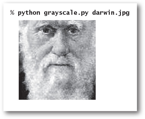
You will find many examples of color images on the booksite, and all of the methods that we describe are effective for full-color images, but all our example images in the text will be grayscale. Accordingly, our first task is to compose a program that can convert images from color to grayscale. This task is a prototypical image-processing task. For each pixel in the source, we have a pixel in the target with a different color. PROGRAM 3.1.5 (grayscale.py) is a filter that takes a file name from the command line and produces a grayscale version of that image. It creates a new Picture object initialized with the color image, then sets the color of each pixel to a new Color having a grayscale value computed by applying the toGray() function in luminance.py (PROGRAM 3.1.4) to the color of the corresponding pixel in the source.
Scaling
One of the most common image-processing tasks is to make an image smaller or larger. Examples of this basic operation, known as scaling, include making small thumbnail photos for use in a chat room or a cellphone, changing the size of a high-resolution photo to make it fit into a specific space in a printed publication or on a web page, or zooming in on a satellite photograph or an image produced by a microscope. In optical systems, we can just move a lens to achieve a desired scale, but in digital imagery, we have to do more work.
In some cases, the strategy is clear. For example, if the target image is to be half the size (in each dimension) of the source image, we simply choose half the pixels—say, by deleting half the rows and half the columns. This technique is known as sampling. If the target image is to be double the size (in each dimension) of the source image, we can replace each source pixel by four target pixels of the same color. Note that we can lose information when we downscale, so halving an image and then doubling it generally does not give back the same image.

A single strategy is effective for both downscaling and upscaling. Our goal is to produce the target image, so we proceed through the pixels in the target, one by one, scaling each pixel’s coordinates to identify a pixel in the source whose color can be assigned to the target. If the width and height of the source are ws and hs, respectively, and the width and height of the target are wt and ht, respectively, then we scale the column index by ws /wt and the row index by hs /ht. That is, we get the color of the pixel in column c and row r of the target from column c×ws/wt and row r×hs/ht in the source. For example, if we are halving the size of a picture, the scale factors are 2, so the pixel in column 4 and row 6 of the target gets the color of the pixel in column 8 and row 12 of the source; if we are doubling the size of the picture, the scale factors are 1/2, so the pixel in column 4 and column 6 of the target gets the color of the pixel in column 2 and row 3 of the source. PROGRAM 3.1.6 (scale.py) is an implementation of this strategy. More sophisticated strategies can be effective for low-resolution images of the sort that you might find on old web pages or from old cameras. For example, we might downscale to half size by averaging the values of four pixels in the source to make one pixel in the target. For the high-resolution images that are common in most applications today, the simple approach used in scale.py is effective.
Program 3.1.5 Converting color to grayscale (grayscale.py)
import sys
import stddraw
import luminance
from picture import Picture
pic = Picture(sys.argv[1])
for col in range(pic.width()):
for row in range(pic.height()):
pixel = pic.get(col, row)
gray = luminance.toGray(pixel)
pic.set(col, row, gray)
stddraw.setCanvasSize(pic.width(), pic.height())
stddraw.picture(pic)
stddraw.show()
pic | image from file
col, row | pixel coordinates
pixel | pixel color
gray | pixel grayscale
This program illustrates a simple image-processing client. First, it creates a Picture object initialized with an image file named by the command-line argument. Then it converts each pixel in the image to grayscale by creating a grayscale version of each pixel’s color and resetting the pixel to that color. Finally, it shows the image. You can perceive individual pixels in the image on the right, which was upscaled from a low-resolution image (see the discussion of scaling starting on the previous page).

The same basic idea of computing the color value of each target pixel as a function of the color values of specific source pixels is effective for all sorts of image-processing tasks. Next, we consider two more examples, and you will find numerous other examples in the exercises and on the booksite.
Fade effect
Our next image-processing example is an entertaining computation where we transform one image to another in a series of discrete steps. Such a transformation is sometimes known as a fade effect. PROGRAM 3.1.7 (fade.py) is a Picture, Color, and stddraw client that uses a linear interpolation strategy to implement this effect. It computes n–1 intermediate images, with each pixel in the tth image being a weighted average of the corresponding pixels in the source and target. The function blend() implements the interpolation: the source color is weighted by a factor of 1 – t / n and the target color by a factor of t / n (when t is 0, we have the source color; when t is n, we have the target color). This simple computation can produce striking results. When you run fade.py on your computer, the change appears to happen dynamically. Try running it on some images from your photo library. Note that fade.py assumes that the images have the same width and height; if you have images for which this is not the case, you can use scale.py to create a scaled version of one or both of them for fade.py.
Program 3.1.6 Image scaling (scale.py)
import sys
import stddraw
from picture import Picture
file = sys.argv[1]
wT = int(sys.argv[2])
hT = int(sys.argv[3])
source = Picture(file)
target = Picture(wT, hT)
for colT in range(wT):
for rowT in range(hT):
colS = colT * source.width() // wT
rowS = rowT * source.height() // hT
target.set(colT, rowT, source.get(colS, rowS))
stddraw.setCanvasSize(wT, hT)
stddraw.picture(target)
stddraw.show()
wT, hT | target dimensions
source | source image
target | target image
colT, rowT | target pixel coords
colS, rowS | source pixel coords
This program accepts the name of either a .jpg or .png image file and two integers wT and hT as command-line arguments and displays the image, scaled to width wT and height hT.

Program 3.1.7 Fade effect (fade.py)
import sys
import stddraw
from color import Color
from picture import Picture
def blend(c1, c2, alpha):
r = (1-alpha)*c1.getRed() + alpha*c2.getRed()
g = (1-alpha)*c1.getGreen() + alpha*c2.getGreen()
b = (1-alpha)*c1.getBlue() + alpha*c2.getBlue()
return Color(int(r), int(g), int(b))
sourceFile = sys.argv[1]
targetFile = sys.argv[2]
n = int(sys.argv[3])
source = Picture(sourceFile)
target = Picture(targetFile)
width = source.width()
height = source.height()
stddraw.setCanvasSize(width, height)
pic = Picture(width, height)
for t in range(n+1):
for col in range(width):
for row in range(height):
c0 = source.get(col, row)
cn = target.get(col, row)
alpha = 1.0 * t / n
pic.set(col, row, blend(c0, cn, alpha))
stddraw.picture(pic)
stddraw.show(1000.0)
stddraw.show()

To fade from one image into another in n-1 intermediate steps, we set each pixel in the tth image to a weighted average of the corresponding pixel in the source and the destination, with the source getting weight 1-t/n and the destination getting weight t/n. The example transformation shown at right is produced by python fade.py mandrill.jpg darwin.jpg 9.
Potential value visualization
Image processing is also helpful in scientific visualization. As an example, we consider a Picture client for visualizing properties of a Charge object—that is, an object of data type Charge as defined at the beginning of this section. PROGRAM 3.1.8 (potential.py) visualizes the potential values created by a set of charged particles. First, potential.py creates an array of particles, with values taken from standard input. Next, it creates a Picture object and sets each pixel in the picture to a shade of gray that is proportional to the potential value at the corresponding point. The calculation at the heart of the approach is very simple: for each pixel, we compute corresponding (x, y) values in the unit square, then call potentialAt() for each charge to find the potential at that point due to all of the charges, summing the values returned. With appropriate assignment of potential values to grayscale values (scaling them to fall between 0 and 255), we get a striking visual representation of the electric potential that is an excellent aid to understanding interactions among such particles. We could produce a similar image using filledSquare() in the stddraw module, but the Picture data type provides us with more accurate control over the color of each pixel on the screen. The same basic approach is useful in many other settings—you can find several examples on the booksite.

It is worthwhile to reflect briefly on the code in potential.py, because it exemplifies data abstraction and object-oriented programming. We want to produce an image that shows interactions among charged particles, and our code reflects precisely the process of creating that image, using a Picture object for the image (which is manipulated via Color objects) and Charge objects for the particles. When we want information about a Charge, we invoke the appropriate method directly for that Charge; when we want to create a Color, we use a Color constructor; when we want to set a pixel, we directly involve the appropriate method for the Picture. These data types are independently developed, but their use together in a single client is easy and natural. We next consider several more examples, to illustrate the broad reach of data abstraction while at the same time adding a number of useful data types to our basic programming model.
Program 3.1.8 Visualizing electric potential (potential.py)
import stddraw
import stdio
import stdarray
from charge import Charge
from color import Color
from picture import Picture
n = stdio.readInt()
charges = stdarray.create1D(n)
for i in range(n):
x0 = stdio.readFloat()
y0 = stdio.readFloat()
q0 = stdio.readFloat()
charges[i] = Charge(x0, y0, q0)
pic = Picture()
for col in range(pic.width()):
for row in range(pic.height()):
x = 1.0 * col / pic.width()
y = 1.0 * row / pic.height()
v = 0.0
for i in range(n):
v += charges[i].potentialAt(x, y)
v = (255 / 2.0) + (v / 2.0e10)
if v < 0: gray = 0
elif v > 255: gray = 255
else: gray = int(v)
color = Color(gray, gray, gray)
pic.set(col, pic.height()-1-row, color)
stddraw.setCanvasSize(pic.width(), pic.height())
stddraw.picture(pic)
stddraw.show()
n | number of charges
charges[] | array of charges
x0, y0 | charge position
q0 | charge value
col, row | pixel position
x, y | point in unit square
gray | scaled potential value
color | pixel color
This program reads values from standard input to create an array of charged particles, sets each pixel color in an image to a grayscale value proportional to the total of the potentials due to the particles at corresponding points, and shows the resulting image.
Input and output revisited
In SECTION 1.5, you learned how to read and write numbers and text using our stdio module. You have certainly come to appreciate the utility of these mechanisms in getting information into and out of your programs. One reason that they are convenient is that the “standard” conventions make them accessible from anywhere within a program. One disadvantage of these conventions is that they leave us dependent upon the operating system’s piping and redirection mechanism for access to files, and they restrict us to working with just one input file and one output file for any given program. With object-oriented programming, we can define mechanisms that are similar to stdio but allow us to work with multiple input streams and output streams within one program.
Specifically, we define in this section the data types InStream and OutStream for input streams and output streams, respectively. As usual, you must make instream.py and outstream.py available to Python, either by putting them in the same directory as your client code or by using your operating system’s path mechanism (see the Q&A at the end of SECTION 2.2).

The purpose of InStream and OutStream is to provide the flexibility that we need to address many common data-processing tasks within our Python programs. Rather than being restricted to just one input stream and one output stream, we can readily create multiple objects of each data type, connecting the streams to various sources and destinations. We also get the flexibility to set variables to reference such objects, pass them as arguments to or return values from functions or methods, and create arrays of them, manipulating them just as we manipulate objects of any data type. We will consider several examples of their use after we have presented the APIs.
Input stream data type
Our data type InStream, defined in the module instream.py, is a more general version of the reading aspects of stdio that supports reading numbers and text from files and websites as well as the standard input stream. The API is shown at the bottom of this page.
Instead of being restricted to one abstract input stream (standard input), this data type gives you the ability to specify directly the source of an input stream. Moreover, that source can be either a file or a website. When you call the InStream constructor with a string argument, the constructor first tries to find a file on your local computer with that name. If it cannot do so, it assumes the argument is a website name and tries to connect to that website. (If no such website exists, it raises an IOError at run time.) In either case, the specified file or website becomes the source of the input for the InStream object thus created, and the read*() methods will read input from that stream.

This arrangement makes it possible to process multiple files within the same program. Moreover, the ability to directly access the web opens up the whole web as potential input for your programs. For example, it allows you to process data that is provided and maintained by someone else. You can find such files all over the web. Scientists now regularly post data files with measurements or results of experiments, ranging from genome and protein sequences to satellite photographs to astronomical observations; financial services companies, such as stock exchanges, regularly publish on the web detailed information about the performance of stock and other financial instruments; governments publish election results; and so forth. Now you can compose Python programs that read these kinds of files directly. The InStream data type gives you a great deal of flexibility to take advantage of the multitude of data sources that are now available.
Output stream data type
Similarly, our data type OutStream, defined in the module outstream.py, is a more general version of the writing aspect of stdio that supports writing strings to a variety of output streams, including standard output and files. Again, the API specifies the same methods as its stdio counterpart. You specify the file that you want to use for output by using the one-argument constructor with the file’s name as argument. OutStream interprets this string as the name of a new file on your local computer, and sends its output there. If you provide no argument to the constructor, then you obtain standard output.

Program 3.1.9 Concatenating files (cat.py)
import sys
from instream import InStream
from outstream import OutStream
inFilenames = sys.argv[1:len(sys.argv)-1]
outFilename = sys.argv[len(sys.argv)-1]
outstream = OutStream(outFilename)
for filename in inFilenames:
instream = InStream(filename)
s = instream.readAll()
outstream.write(s)
outstream | output stream
filename | current file name
instream | current input stream
s | contents of filename
This program creates an output file whose name is given by the last command-line argument and whose contents are copies of the input files whose names are given as the other arguments.
% more in1.txt
This is
% more in2.txt
a tiny
test.
% python cat.py in1.txt in2.txt out.txt
% more out.txt
This is
a tiny
test.
File concatenation and filtering
PROGRAM 3.1.9 (cat.py) is a sample client of InStream and OutStream that uses multiple input streams to concatenate several input files into a single output file. Some operating systems have a command known as cat that implements this function. However, a Python program that does the same thing is perhaps more useful, because we can tailor it to filter the input files in various ways: we might wish to ignore irrelevant information, change the format, or select only some of the data, to name just a few examples. We now consider one example of such processing, and you can find several others in the exercises.
Screen scraping
The combination of InStream (which allows us to create an input stream from any page on the web) and str (which provides powerful tools for processing text strings) opens up the entire web to direct access by our Python programs, without any direct dependence on the operating system or the browser. One paradigm is known as screen scraping: the goal is to extract some information from a web page with a program rather than having to browse to find it. To do so, we take advantage of the fact that many web pages are defined with text files in a highly structured format (because they are created by computer programs!). Your browser has a mechanism that allows you to examine the source code that produces the web page that you are viewing, and by examining that source you can often figure out what to do.
...
(GOOG)</h2> <span class="rtq_
exch"><span class="rtq_dash">-</span>
NMS </span><span class="wl_sign">
</span></div></div>
<div class="yfi_rt_quote_summary_rt_top
sigfig_promo_1"><div>
<span class="time_rtq_ticker">
<span id="yfs_l84goog">1,100.62</span>
</span> <span class="down_r time_rtq_
content"><span id="yfs_c63_goog">
...
HTML code from the web
Suppose that we want to take a stock trading symbol as a command-line argument and write out its current trading price. Such information is published on the web by financial service companies and internet service providers. For example, you can find the stock price of a company whose symbol is goog by browsing to http://finance.yahoo.com/q?s=goog. Like many web pages, the name encodes an argument (goog), and we could substitute any other ticker symbol to get a web page with financial information for any other company. Also, like many other files on the web, the referenced file is a text file, written in a formatting language known as HTML. From the point of view of a Python program, it is just a str value accessible through an InStream object. You can use your browser to download the source of that file, or you could use
python cat.py "http://finance.yahoo.com/q?s=goog" mycopy.txt
to put the source into a local file mycopy.txt on your computer (though there is no real need to do so). Now, suppose that goog is trading at $1,100.62 at the moment. If you search for the string '1,100.62' in the source of that page, you will find the stock price buried within some HTML code. Without having to know details of HTML, you can figure out something about the context in which the price appears. In this case, you can see that the stock price is enclosed between the substrings <span id="yfs_l84goog"> and </span>.
Program 3.1.10 Screen scraping for stock quotes (stockquote.py)
import sys
import stdio
from instream import InStream
def _readHTML(stockSymbol):
WEBSITE = 'http://finance.yahoo.com/q?s='
page = InStream(WEBSITE + stockSymbol)
html = page.readAll()
return html
def priceOf(stockSymbol):
html = _readHTML(stockSymbol)
trade = html.find('yfs_l84', 0)
beg = html.find('>', trade)
end = html.find('</span>', beg)
price = html[beg+1:end]
price = price.replace(',', '')
return float(price)
def main():
stockSymbol = sys.argv[1]
price = priceOf(stockSymbol)
stdio.writef('%.2f
', price)
if __name__ == '__main__': main()
page | input stream
html | contents of page
trade | yfs_l84 index
beg | > after trade index
end | </span> after to index
price | current price
This program accepts a stock ticker symbol as a command-line argument and writes to standard output the current stock price for that stock, as reported by the website http://finance.yahoo.com. It uses string slicing and the find() and replace() methods from str.
% python stockquote.py goog
1100.62
% python stockquote.py adbe
70.51
With the str data type’s find() method and string slicing, you easily can grab this information, as illustrated in stockquote.py (PROGRAM 3.1.10). This program depends on the web page format used by http://finance.yahoo.com; if this format changes, stockquote.py will not work. Indeed, by the time you read this page, the format may have changed. Still, making appropriate changes is not likely to be difficult. You can entertain yourself by embellishing stockquote.py in all kinds of interesting ways. For example, you could grab the stock price on a periodic basis and plot it, compute a moving average, or save the results to a file for later analysis. Of course, the same technique works for sources of data found all over the web, as you can see in examples in the exercises at the end of this section and on the booksite.
Extracting data
The ability to maintain multiple input and output streams gives us a great deal of flexibility in meeting the challenges of processing large amounts of data coming from a variety of sources. We now consider one more example. Suppose that a scientist or a financial analyst has a large amount of data within a spreadsheet program. Typically such spreadsheets are tables with a relatively large number of rows and a relatively small number of columns. You are not likely to be interested in all the data in the spreadsheet, but you may be interested in a few of the columns. You can do some calculations within the spreadsheet program (this is its purpose, after all), but you certainly do not have the flexibility that you can realize with Python programming. One way to address this situation is to have the spreadsheet export the data to a text file, using some special character to delimit the columns, and then compose a Python program that reads the file from an input stream. One standard practice is to use commas as delimiters: write one line per row, with commas separating column entries. Such files are known as comma-separated-value or .csv files. With the split() method in Python’s str data type, we can read the file line-by-line and isolate the data that we want. We will see several examples of this approach later in the book. PROGRAM 3.1.11 (split.py) is an InStream and OutStream client that goes one step further: it creates multiple output streams and makes one file for each column.
These examples are convincing illustrations of the utility of working with text files, with multiple input and output streams, and with direct access to web pages. Web pages are written in HTML precisely so that they will be accessible to any program that can read strings. People use text formats such as .csv files rather than data formats that are beholden to particular applications precisely to allow as many people as possible to access the data with simple programs like split.py.
Program 3.1.11 Splitting a file (split.py)
import sys
import stdarray
from instream import InStream
from outstream import OutStream
basename = sys.argv[1]
n = int(sys.argv[2])
instream = InStream(basename + '.csv')
out = stdarray.create1D(n)
for i in range(n):
out[i] = OutStream(basename + str(i) + '.txt')
while instream.hasNextLine():
line = instream.readLine()
fields = line.split(',')
for i in range(n):
out[i].writeln(fields[i])
basename | base file name
n | number of fields
instream | input stream
out[] | output streams
line | current line
fields[] | values in current line
This program uses multiple output streams to split a .csv file into separate files, one for each comma-delimited field. It accepts a string basename and an integer n as command-line arguments and splits the file whose name is basename.csv, by field (comma-separated), into n files named basename0.txt, basename1.txt, and so forth.
% more djia.csv
...
31-Oct-29,264.97,7150000,273.51
30-Oct-29,230.98,10730000,258.47
29-Oct-29,252.38,16410000,230.07
28-Oct-29,295.18,9210000,260.64
25-Oct-29,299.47,5920000,301.22
24-Oct-29,305.85,12900000,299.47
23-Oct-29,326.51,6370000,305.85
22-Oct-29,322.03,4130000,326.51
21-Oct-29,323.87,6090000,320.91
...
% python split.py djia 4
% more djia2.txt
...
7150000
10730000
16410000
9210000
5920000
12900000
6370000
4130000
6090000
...
Memory management
Now that you have seen several examples of object-oriented data types (str, Charge, Color, Picture, InStream, and Outstream) and client programs that use them, we can discuss in more detail the challenges Python faces in providing support for such programs. To a large extent, Python protects novice programmers from having to know these details, but having some idea of what is going on inside the system is sometimes helpful in writing correct, effective, and efficient object-oriented programs.
In Python, we create objects by calling a constructor. Each time we create an object, Python reserves computer memory for that object. But when and how do we destroy objects so that the memory in which they reside can be freed for reuse? We will briefly address this question.
Orphaned objects
The ability to bind a variable to a different object creates the possibility that a program may have created an object that it can no longer reference. For example, consider the three assignment statements in the figure at right. After the third assignment statement, not only do c1 and c2 refer to the same Charge object (the one at (.51, .63) with potential 21.3), but there is also no longer a reference to the Charge object that was created and used to initialize c2. The only reference to that object was in the variable c2, and this reference was overwritten by the assignment, so there is no way to refer to the object again. Such an object is said to be an orphan. Objects can also become orphans when variables go out of scope. Python programmers pay little attention to orphaned objects because the system automatically reuses the memory that they occupy, as we discuss next.

Memory management
Programs tend to create huge numbers of objects but have a need for only a small number of them at any given time. Accordingly, programming languages and systems need mechanisms to create objects (and allocate memory), and mechanisms to destroy objects (and free memory) when the objects become orphans. Most programming systems take care of allocating memory for variables when they come into existence and freeing that memory when they go out of scope. Memory management for objects is more complicated: Python knows to allocate memory for an object when it is created, but cannot know precisely when to free the memory associated with an object, because the dynamics of a program in execution determine when an object becomes an orphan and so should be destroyed. There is no way for the system to predict what a program will do, so it has to monitor what a program is doing and take action accordingly.
Memory leaks
In many languages (such as C and C++), the programmer is responsible for both allocating and deallocating memory. Doing so is tedious and notoriously error-prone. For example, suppose that a program deallocates the memory for an object, but then continues to refer to it (perhaps much later in the program). In the meantime, the system may have reallocated the same memory for another use, so all kinds of havoc can result. Another insidious problem occurs when a programmer neglects to ensure that the memory for an orphaned object is deallocated. This bug is known as a memory leak because it can result in a steadily increasing amount of memory devoted to orphaned objects (and therefore not available for use). The effect is that performance degrades, just as if memory were leaking out of your computer. Have you ever had to reboot your computer because it was gradually getting less and less responsive? A common cause of such behavior is a memory leak in one of your applications.
Garbage collection
One of Python’s most significant features is its ability to automatically manage memory. The idea is to free the programmers from the responsibility of managing memory by keeping track of orphaned objects and returning the memory they use to a pool of free memory. Reclaiming memory in this way is known as garbage collection, and Python’s type system enables it to perform this operation this efficiently and automatically. Garbage collection is an old idea, and some people still debate whether the overhead of automatic garbage collection justifies the convenience of not having to worry about memory management. But many other people (including Python and Java programmers, for example) very much enjoy the benefits of not having to worry about memory management and memory leaks.
For reference, we summarize the data types that we have considered in this section in the table at right. We chose these examples to help you understand the essential properties of data types and object-oriented programming.
A data type is a set of values and a set of operations defined on those values. With built-in numeric types, we worked with a small and simple set of values. Colors, pictures, strings, and input/output streams are high-level data types that indicate the breadth of applicability of data abstraction. You do not need to know how a data type is implemented to be able to use it. Each data type (there are hundreds in Python’s standard and extension modules, and you will soon learn to create your own) is characterized by an API (application programming interface) that provides the information that you need to use it. A client program creates objects that hold data-type values and calls methods to manipulate those values. We compose client programs with the basic statements and control structures that you learned in CHAPTERS 1 and 2, but now have the capability to work with a vast variety of data types, not just the built-in ones to which you have grown accustomed. With experience, you will find that this ability opens up new horizons in programming.

Our Charge example demonstrated that you can tailor one or more data types to the needs of your application. The ability to do so is a profound benefit, and also is the subject of the next section. When properly designed and implemented, data types lead to client programs that are clearer, easier to develop, and easier to maintain than equivalent programs that do not take advantage of data abstraction. The client programs in this section are testimony to this claim. Moreover, as you will see in the next section, implementing a data type is a straightforward application of the basic programming skills that you have already learned. In particular, addressing a large and complex application becomes a process of understanding its data and the operations to be performed on it, then composing programs that directly reflect this understanding. Once you have learned to do so, you might wonder how programmers ever developed large programs without using data abstraction.
A. Python raises an AttributeError at run time.
Q. Why can we use stdio.writeln(x) instead of stdio.writeln(str(x)) to write an object x that is not a string?
A. For convenience, the stdio.writeln() function calls the built-in str() function automatically whenever a string object is needed.
Q. I noticed that potential.py (PROGRAM 3.1.8) calls stdarray.create1D() to create an array of Charge objects, but provides only one argument (the desired number of elements). Doesn’t stdarray.create1D() require that I provide two arguments: the desired number of elements and the initial value of the elements?
A. If no initial value is specified, both stddarray.create1D() and stdarray.create2D() use the special value None, which refers to no object. Immediately after calling stdarray.create1D(), potential.py changes each array element so it refers to a new Charge object.
Q. Can I call a method with a literal or other expression?
A. Yes, from the client’s point of view, you can use any expression to invoke a method. When Python executes the method call, it evaluates the expression and calls the method on the resulting object. For example, 'python'.upper() returns ‘Python' and (3 ** 100).bit_length() returns 159. However, you need to be careful with integer literals—for example, 1023.bit_length() raises a SyntaxError because Python interprets 1023. as a floating-point literal; instead, you can use (1023).bit_length().
Q. Can I chain together several string method calls in one expression?
A. Yes. For example, the expression s.strip().lower() works as expected. That is, it evaluates to a new string that is a copy of s with leading and trailing whitespace removed, and with all remaining characters converted to lowercase. It works because (1) each of the methods returns its result as a string and (2) the dot operator is left associative, so Python calls the methods from left to right.
Q. Why red, green, and blue instead of red, yellow, and blue?
A. In theory, any three colors that contain some amount of each primary color would work, but two different color models have evolved: RGB produces good colors on television screens, computer monitors, and digital cameras, and CMYK is typically used for the printed page (see EXERCISE 1.2.28). CMYK does include yellow (cyan, magenta, yellow, and black). Two different schemes are appropriate because printed inks absorb color; thus, where there are two different inks, there are more colors absorbed and fewer reflected. In contrast, video displays emit color; thus, where there are two different colored pixels, there are more colors emitted.
Q. Is there any problem with creating thousands of Color objects, as in grayscale.py (PROGRAM 3.1.5)? It seems wasteful.
A. All programming-language constructs come at some cost. In this case the cost is reasonable, since the time required to create the Color objects is tiny compared to the time required to actually draw the picture.
Q. Can a data type have two methods (or constructors) with the same name but with a different number of arguments?
A. No, just as with functions, you cannot have two methods (or constructors) with the same name. As with functions, methods (and constructors) can use optional arguments with default values. This is how the Picture data type creates the illusion of having two constructors.
Exercises
3.1.1 Compose a program that takes a float command-line argument w, creates four Charge objects that are each distance w in each of the four cardinal directions from (0.5, 0.5), and writes the potential at (0.25, 0.5).
3.1.2 Compose a program that takes from the command line three integers between 0 and 255 that represent red, green, and blue values of a color and then creates and shows a 256-by-256 Picture of that color.
3.1.3 Modify alberssquares.py (PROGRAM 3.1.3) to take nine command-line arguments that specify three colors and then draw the six squares showing all the Albers squares with the large square in each color and the small square in each different color.
3.1.4 Compose a program that takes the name of a grayscale picture file as a command-line argument and uses stddraw to plot a histogram of the frequency of occurrence of each of the 256 grayscale intensities.
3.1.5 Compose a program that takes the name of a picture file as a command-line argument and flips the image horizontally.
3.1.6 Compose a program that takes the name of a picture file as a command-line input, and creates three images—one with only the red components, one with only the green components, and one with only the blue components.
3.1.7 Compose a program that takes the name of a picture file as a command-line argument and writes the pixel coordinates of the lower-left corner and the upper-right corner of the smallest bounding box (rectangle parallel to the x- and y-axes) that contains all of the non-white pixels.
3.1.8 Compose a program that takes as command-line arguments the name of a picture file and the pixel coordinates of a rectangle within the image; reads from standard input a list of Color values (represented as triples of integers); and serves as a filter, writing those Color values for which all pixels in the rectangle are background/foreground compatible. (Such a filter can be used to pick a color for text to label an image.)
3.1.9 Compose a function isValidDNA() that takes a string as its argument and returns True if and only if it consists entirely of the characters A, C, T, and G.
3.1.10 Compose a function complementWC() that takes a DNA string as its argument and returns its Watson–Crick complement: replace A with T, and C with G, and vice versa.
3.1.11 Compose a function palindromeWC() that takes a DNA string as its argument and returns True if the string is a Watson–Crick complemented palindrome, and False otherwise. A Watson–Crick complemented palindrome is a DNA string that is equal to the reverse of its Watson–Crick complement.
3.1.12 Compose a program to check whether an ISBN number is valid (see EXERCISE 1.3.33), taking into account that an ISBN number can have hyphens inserted at arbitrary places.
3.1.13 What does the following code fragment write?
s = 'Hello World'
s.upper()
s[6:11]
stdio.writeln(s)
Solution: 'Hello World'. String objects are immutable—a string method returns a new str object with the appropriate value, but does not change the value of the string that was used to invoke it. Therefore, this code ignores the objects returned and just writes the original string. To update s, write s = s.upper() and s = s[6:11].
3.1.14 A string s is a circular shift of a string t if it matches when the characters are circularly shifted by any number of positions. For example, ACTGACG is a circular shift of TGACGAC, and vice versa. Detecting this condition is important in the study of genomic sequences. Compose a function that checks whether two given strings s and t are circular shifts of one another. Hint: The solution is a one-liner with the in operator and string concatenation.
3.1.15 Given a string that represents a website URL, compose a code fragment that determines its domain type. For example, the domain type for our booksite URL http://introcs.cs.princeton.edu/python is edu.
3.1.16 Compose a function that takes a domain name as an argument and returns the reverse domain (reverse the order of the strings between periods). For example, the reverse domain of introcs.cs.princeton.edu is edu.princeton.cs.introcs. This computation is useful for web log analysis. (See EXERCISE 4.2.33.)
3.1.17 What does the following recursive function return?
def mystery(s):
n = len(s)
if (n <= 1): return s
a = s[0 : n//2]
b = s[n//2 : n]
return mystery(b) + mystery(a)
3.1.18 Compose a version of potentialgene.py (PROGRAM 3.1.1) that finds all potential genes contained in a long DNA string. Add a command-line argument to allow the user to specify a minimum length of a potential gene.
3.1.19 Compose a program that takes a start string and a stop string as command-line arguments and writes all substrings of a given string that start with the first, end with the second, and otherwise contain neither. Note: Be especially careful of overlaps!
3.1.20 Compose a filter that reads text from an input stream and writes it to an output stream, removing any lines that consist only of whitespace.
3.1.21 Modify potential.py (PROGRAM 3.1.8) to take an integer n from the command line and generate n random Charge objects in the unit square, with potential values drawn randomly from a Gaussian distribution with mean 50 and standard deviation 10.
3.1.22 Modify stockquote.py (PROGRAM 3.1.10) to take multiple symbols on the command line.
3.1.23 The example file djia.csv used for split.py (PROGRAM 3.1.11) lists the date, high price, volume, and low price of the Dow Jones stock market average for every day since records have been kept. Download this file from the booksite and compose a program that plots the prices and volumes, at a rate taken from the command line.
3.1.24 Compose a program merge.py that takes a delimiter string followed by an arbitrary number of file names as command-line arguments; concatenates the corresponding lines of each file, separated by the delimiter; and then writes the result to standard output, thus performing the opposite operation from split.py (PROGRAM 3.1.11).
3.1.25 Find a website that publishes the current temperature in your area, and write a screen-scraper program weather.py so that typing python weather.py followed by your ZIP code will give you a weather forecast.
Creative Exercises
3.1.26 Picture filtering. Compose a module rawpicture.py with read() and write() functions for use with standard input and standard output. The write() function takes a Picture as argument and writes the picture to standard output, using the following format: if the picture is w-by-h, write w, then h, then w*h triples of integers representing the pixel color values, in row-major order. The read() function takes no arguments and returns a Picture, which it creates by reading a picture from standard input, in the format just described. Note: The picture filtering will use up much more disk space than the picture—the standard formats compress this information so that it will not take up so much space.
3.1.27 Kama Sutra cipher. Compose a filter KamaSutra that takes two strings as command-line argument (the key strings), then reads standard input, substitutes for each letter as specified by the key strings, and writes the result to standard output. This operation is the basis for one of the earliest known cryptographic systems. The condition on the key strings is that they must be of equal length and that any letter in standard input must be in one of them. For example, if input is all capitals and the keys are THEQUICKBROWN and FXJMPSVRLZYDG, then we make this table:
T H E Q U I C K B R O W N
F X J M P S V L A Z Y D G
That is, we should substitute F for T, T for F, H for X, X for H, and so forth when copying the input to the output. The message is encoded by replacing each letter with its pair. For example, the message MEET AT ELEVEN is encoded as QJJF BF JKJCJG. Someone receiving the message can use the same keys to get the message back.
3.1.28 Safe password verification. Compose a function that takes a string as an argument and returns True if it meets the following conditions, False otherwise:
• At least eight characters long
• Contains at least one digit (0–9)
• Contains at least one uppercase letter
• Contains at least one lowercase letter
• Contains at least one character that is neither a letter nor a number
Such checks are commonly used for passwords on the web.
3.1.29 Sound visualization. Compose a program that uses stdaudio and Picture to create an interesting two-dimensional color visualization of a sound file while it is playing. Be creative!
3.1.30 Color study. Compose a program that displays the color study shown at right, which gives Albers squares corresponding to each of the 256 levels of blue (blue-to-white in row-major order) and gray (black-to-white in column-major order) that were used to print this book.
3.1.31 Entropy. The Shannon entropy measures the information content of an input string and plays a cornerstone role in information theory and data compression. Given a string of n characters, let fc be the frequency of occurrence of character c. The quantity pc = fc / n is an estimate of the probability that c would be in the string if it were a random string, and the entropy is defined to be the sum of the quantity –pc log2 pc, over all characters that appear in the string. The entropy is said to measure the information content of a string: if each character appears the same number of times, the entropy is at its minimum value. Compose a program that computes and writes to standard output the entropy of the string read from standard input. Run your program on a web page that you read regularly, on a recent paper that you wrote, and on the fruit fly genome found on the website.
3.1.32 Minimize potential. Compose a function that takes an array of Charge objects with positive potential as its argument and finds a point such that the potential at that point is within 1% of the minimum potential anywhere in the unit square. Compose a test client that calls your function to write the point coordinates and charge value for the data given in the text and for the random charges described in EXERCISE 3.1.21.

3.1.33 Slide show. Compose a program that takes the names of several image files as command-line arguments and displays them in a slide show (one every two seconds), using a fade effect to black and a fade from black between pictures.
3.1.34 Tile. Compose a program that takes the name of an image file and two integers m and n as command-line arguments and creates an m-by-n tiling of the picture.
3.1.35 Rotation filter. Compose a program that takes two command-line arguments (the name of an image file and a real number theta) and rotates the image θ degrees counterclockwise. To rotate, copy the color of each pixel (si, s j) in the source image to a target pixel (ti, t j) whose coordinates are given by the following formulas:
ti = (si – ci)cos θ – (sj – cj)sin θ + ci
tj = (si – ci)sin θ + (sj – cj)cos θ + cj
where (c i, c j) is the center of the image.
3.1.36 Swirl filter. Creating a swirl effect is similar to rotation, except that the angle changes as a function of distance to the center. Use the same formulas as in the previous exercise, but compute θ as a function of (si, s j)—specifically, π / 256 times the distance to the center.
3.1.37 Wave filter. Compose a filter like those in the previous two exercises that creates a wave effect, by copying the color of each pixel (si, s j) in the source image to a target pixel (ti, t j), where ti = si and tj = sj +20 sin(2 π si /64). Add code to take the amplitude (20 in the accompanying figure) and the frequency (64 in the accompanying figure) as command-line arguments. Experiment with various values of these parameters.
3.1.38 Glass filter. Compose a program that takes the name of an image file as a command-line argument and applies a glass filter: set each pixel p to the color of a random neighboring pixel (whose pixel coordinates are each within 5 pixels of p’s coordinates).
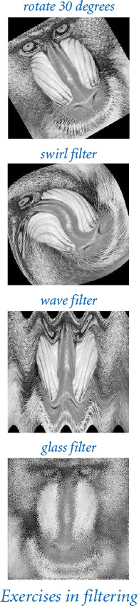
3.1.39 Morph. The example images in the text for fade.py do not quite line up in the vertical direction (the mandrill’s mouth is much lower than Darwin’s mouth). Modify fade.py to add a transformation in the vertical dimension that makes a smoother transition.
3.1.40 Clusters. Compose a program that takes the name of a picture file from the command line and produces and displays to stddraw a picture with filled circles that cover compatible areas. First, scan the image to determine the background color (a dominant color that is found in more than half the pixels). Use a depth-first search (see PROGRAM 2.4.6) to find contiguous sets of pixels that are foreground-compatible with the background. A scientist might use a program to study natural scenarios such as birds in flight or particles in motion. Take a photo of balls on a billiards table and try to get your program to identify the balls and positions.
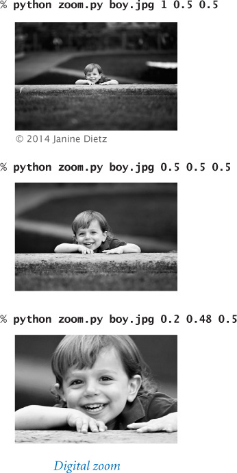
3.1.41 Digital zoom. Compose a program zoom.py that takes the name of a picture file and three floats s, x, and y as command-line arguments and displays a picture that zooms in on a portion of the input picture. The numbers should all be between 0 and 1, with s to be interpreted as a scale factor and (x, y) as the relative coordinates of the point that is to be at the center of the output image. Use this program to zoom in on your pet, friend, or relative in some digital image on your computer.
3.2 Creating Data Types
In principle, we could compose all of our programs using only built-in data types. However, as we saw in the last section, it is much more convenient to compose programs at a higher level of abstraction. Thus, many other data types are defined in Python’s standard and extension modules. Still, we certainly cannot expect those modules to define every conceivable data type that we might ever wish to use, so we need to be able to define our own. The purpose of this section is to explain how to build our own data types in Python.
Programs in this section
A data type is a set of values and a set of operations defined on those values. In Python, we implement a data type using a class. The API specifies the operations that we need to implement, but we are free to choose any convenient representation for the values. Implementing a data type as a Python class is not very different from implementing a function module as a set of functions. The primary differences are that we associate values (in the form of instance variables) with methods and that each method call is associated with the object used to invoke it.
To cement the basic concepts, we begin by defining a class that implements the data type for charged particles that we introduced in SECTION 3.1. Then, we illustrate the process of defining classes by considering a range of examples, from complex numbers to stock accounts, including a number of software tools that we will use later in the book. Useful client code is testimony to the value of any data type, so we also consider a number of clients, including one that depicts the famous and fascinating Mandelbrot set.
The process of defining a data type is known as data abstraction (as opposed to the function abstraction style that is the basis of CHAPTER 2). We focus on the data and implement operations on that data. Whenever you can clearly separate data and associated operations within a computation, you should do so. Modeling physical objects or mathematical abstractions is straightforward and useful, but the true power of data abstraction is that it allows us to model anything that we can precisely specify. Once you gain experience with this style of programming, you will see that it naturally helps address programming challenges of arbitrary complexity.
Basic elements of a data type
To illustrate the process of implementing a data type as a Python class, we now consider an implementation of the Charge data type of SECTION 3.1 in full detail. We have already considered client programs that demonstrate the utility of having such a data type (in PROGRAM 3.1.2 and PROGRAM 3.1.8); now we focus on the implementation details. Every data-type implementation that you will develop has the same basic ingredients as this example.
API
The application programming interface is the contract with all clients and, therefore, the starting point for any implementation. To emphasize that APIs are critical for implementations, we repeat below the Charge API. To implement the Charge data type as a Python class, we need to define the data-type values, compose code to initialize new Charge objects with specified data-type values, and implement two methods that manipulate those values. When faced with the problem of creating a completely new data type for some application, the first step is to develop an API. This step is a design activity that we will address in SECTION 3.3. We have already looked at APIs as specifications of how to use data types in client code; now look at them as specifications of how to implement data types.
Class
In Python, we implement a data type as a class. As we have seen, Python’s convention is to put the code for a data type in a file with the same name as the class, but in lowercase and followed by the .py extension. Thus, we keep the code for Charge in a file named charge.py. To define a class, you use the keyword class, followed by the class name, followed by a colon, and then a list of method definitions. Our class adheres to conventions that define three key features of a data type: a constructor, instance variables, and methods, which we will address in detail next. Since these features are intertwined, the discussion is a bit circular at points, so a good strategy is to read all three descriptions, then reread them.

Constructor
A constructor creates an object of the specified type and returns a reference to that object. For our example, the client code
c = Charge(x0, y0, q0)
returns a new Charge object, suitably initialized. Python provides a flexible and general mechanism for object creation, but we adopt a simple subset that well serves our style of programming. Specifically, in this book, each data type defines a special method __init__() whose purpose is to define and initialize the instance variables, as described below. The double underscores before and after the name are your clue that it is “special”—we will be encountering other special methods soon.
When a client calls a constructor, Python’s default construction process creates a new object of the specified type, calls the __init__() method to define and initialize the instance variables, and returns a reference to the new object. In this book, we refer to __init__() as the constructor for the data type, even though it is technically only the pertinent part of the object-creation process.
The code at right is the __init__() implementation for Charge. It is a method, so its first line is a signature consisting of the keyword def, its name (__init__), a list of parameter variables, and a colon. By convention, the first parameter variable is named self. As part of Python’s default object creation process, the value of the self parameter variable when __init()__ is invoked is a reference to the newly created object. The ordinary parameter variables from the client follow the special parameter variable self. The remaining lines make up the body of the constructor. Our convention throughout this book is for __init()__ to consist of code that initializes the newly created object by defining and initializing the instance variables.

Instance variables
A data type is a set of values and a set of operations defined on those values. In Python, instance variables implement the values. An instance variable belongs to a particular instance of a class—that is, to a particular object. In this book, our convention is to define and initialize each instance variable of the newly created object in the constructor and only in the constructor. The standard convention in Python programs is that instance variable names begin with an underscore. In our implementations, you can inspect the constructor to see the entire set of instance variables. For example, the __init__() implementation on the previous page tells us that Charge has three instance variables _rx, _ry, and _q. When an object is created, the value of the self parameter variable of the __init__() method is a reference to that object. Just as we can call a method for a charge c with the syntax c.potentialAt(), so we can refer to an instance variable for a charge self with the syntax self._rx. Therefore the three lines within the __init__() constructor for Charge define and initialize _rx, _ry, and _q for the new object.
Details of object creation
The memory diagrams at right detail the precise sequence of events when a client creates a new Charge object with the code
c1 = Charge(0.51, 0.63, 21.3)
• Python creates the object and calls the __init__() constructor, initializing the constructor’s self parameter variable to reference the newly created object, its x0 parameter variable to reference 0.51, its y0 parameter variable to reference 0.63, and its q0 parameter variable to reference 21.3.
• The constructor defines and initializes the _rx, _ry, and _q instance variables within the newly created object referenced by self.
• After the constructor finishes, Python automatically returns to the client the self reference to the newly created object.
• The client assigns that reference to c1.

The parameter variables x0, y0, and q0 go out of scope when __init__() is finished, but the objects they reference are still accessible via the new object’s instance variables.
Methods
A data type is a set of values and a set of operations defined on those values. In Python, methods (or instance methods) implement data-type operations, which are associated with a specified object. To define methods, we compose code that is precisely like the code that we learned in CHAPTER 2 to define functions, with the (significant) exception that methods can also access instance variables. For example, the code of the potentialAt() method for our Charge data type is shown below. The first line is the method’s signature: the keyword def, the name of the method, parameter variables names in parentheses, and a colon. The first parameter variable of every method is named self. When a client calls a method, Python automatically sets that self parameter variable to reference the object to be manipulated—the object that was used to invoke the method. For example, when a client calls our method with c.potentialAt(x, y), the value of the self parameter variable of the __potentialAt__() method is set to c. The ordinary parameter variables from the client (x and y, in this case) follow the special parameter variable self. The remaining lines make up the body of the potentialAt() method.

Variables within methods
To understand method implementations, it is very important to know that a method typically uses three kinds of variables:
• The self object’s instance variables
• The method’s parameter variables
• Local variables
There is a critical distinction between instance variables and the parameter and local variables that you are accustomed to: there is just one value corresponding to each local or parameter variable at a given time, but there can be many values corresponding to each instance variable—one for each object that is an instance of the data type. There is no ambiguity with this arrangement, because each time that you call a method, you use an object to do so, and the implementation code

can directly refer to that object’s instance variables using the self parameter variable. Be sure that you understand the distinctions among these three kinds of variables. The differences are summarized in table above, and are a key to object-oriented programming. In our example, potentialAt() uses the _rx, _ry, and _q instance variables of the object referenced by self, the parameter variables x and y, and the local variables COULOMB, dx, dy, and r to compute and return a value. As an example, note that the statement
dx = x - self._rx
uses all three kinds of variables. With these distinctions in mind, check that you understand how potentialAt() gets its job done.
Methods are functions
A method is a special kind of function that is defined in a class and associated with an object. Since methods are functions, a method can take any number of arguments, specify optional arguments with default values, and return a value to its caller. In our example, potentialAt() takes two ordinary arguments and returns a float to the client. The key difference between functions and methods is that a method is associated with a specified object, with direct access to its instance variables. Indeed, we will see examples later in this section where the purpose of a method is to have the side effect of changing an instance variable, rather than returning a value to the client.
Built-in functions
The third operation in the Charge API is a built-in function str(c). Python’s convention is to automatically translate this function call to a standard method call c.__str()__. Thus, to support this operation, we implement the special method __str__(), which uses the instance variables associated with the invoking object to string together the desired result. Recall that Python knows the type of each object at run time, so Python can infer which __str__() method to call—the one defined in the class corresponding to the invoking object.
Privacy
A client should access a data type only through the methods in its API. Sometimes it is convenient to define helper methods in the implementation that are not intended to be called directly by the client. The special method __str__() is a prototypical example. As we saw in SECTION 2.2 with private functions, the standard Python convention is to name such methods with a leading underscore. The leading underscore is a strong signal to the client not to call that private method directly. Similarly, naming instance variables with a leading underscore signals to the client not to access such private instance variables directly. Even though Python has no language support for enforcing these conventions, most Python programmers treat them as sacrosanct.
These are the basic components that you must understand to implement data types as classes in Python. Every data-type implementation (Python class) that we will consider has instance variables, constructors, and methods. In each data type that we develop, we go through the same steps. Rather than thinking about which action we need to take next to accomplish a computational goal (as we did when first learning to program), we think about the needs of a client, then accommodate them in a data type. PROGRAM 3.2.1 is a full implementation of our Charge data type; it illustrates all of the features we have just discussed. Note that charge.py also has a test client. As with modules, it is good style to include a test client with every data-type implementation.
Summary
At the risk of being repetitive, we summarize the basic steps that we have described in the process of creating a new data type.
The first step in creating a data type is to specify an API. The purpose of the API is to separate clients from implementations, thereby facilitating modular programming. We have two goals when specifying an API. First, we want to enable clear and correct client code. Indeed, it is a good idea to compose some client code before finalizing the API to gain confidence that the specified data-type operations are the ones that clients need. Second, we need to be able to implement the operations. There is no point in specifying operations that we have no idea how to implement.
The second step in creating a data type is to implement a Python class that meets the API specifications. First, we compose the constructor to define and initialize the instance variables; then, we compose the methods that manipulate the instance variables to implement the desired functionality. In Python, we normally need to implement three kinds of methods:
Program 3.2.1 Charged particle (charge.py)
import math
import sys
import stdio
class Charge:
def __init__(self, x0, y0, q0):
self._rx = x0
self._ry = y0
self._q = q0
def potentialAt(self, x, y):
COULOMB = 8.99e09
dx = x - self._rx
dy = y - self._ry
r = math.sqrt(dx*dx + dy*dy)
if r == 0.0: return float('inf')
return COULOMB * self._q / r
def __str__(self):
result = str(self._q) + ' at ('
result += str(self._rx) + ', ' + str(self._ry) + ')'
return result
def main():
x = float(sys.argv[1])
y = float(sys.argv[2])
c = Charge(.51, .63, 21.3)
stdio.writeln(c)
stdio.writeln(c.potentialAt(x, y))
if __name__ == '__main__': main()
instance variables
_rx | x-coordinate
_ry | y-coordinate
_q | charge value
COULOMB | Coulomb's constant
dx, dy | delta distances to query point
r | distance to query point
x, y | query point
c | charge
This implementation of our data type for charged particles contains the basic ingredients found in every data type: instance variables _rx, _ry, and _q; a constructor __init__(); the methods potentialAt() and __str__(); and a test client main() (see also PROGRAM 3.1.1).
% python charge.py .5 .5
21.3 at (0.51, 0.63)
1468638248194.164
• To implement a constructor, we implement a special method __init__() with self as its first parameter variable, followed by the constructor’s ordinary parameter variables.
• To implement a method, we implement a function of the desired name, with self as its first parameter variable, followed by the method’s ordinary parameter variables.
• To implement a built-in function, we implement a special method with the same name enclosed in double underscores and with self as its first parameter variable.
Examples from Charge are shown in the table at the bottom of this page. In all three cases, we use self to access the instance variables of the invoking object and otherwise use parameter and local variables to compute a result and return a value to the caller.
The third step in creating a data type is to compose a test client, to validate and test the design decisions made in the first two steps.
The diagram on the facing page summarizes the terminology that we have discussed. It is well worth careful study, as we will be using this terminology extensively for the rest of the book.
For the rest of this section, we apply these basic steps to create a number of interesting data types and clients. We start each example with an API, and then consider implementations, followed by clients. You will find many exercises at the end of this section intended to give you experience with data-type creation. SECTION 3.3 provides an overview of the design process and related language mechanisms.
What are the values that define the data type, and which operations do clients need to perform on those values? With these basic decisions made, you can create new data types and compose clients that use them in the same way as you have been using built-in data types.


Stopwatch
One of the hallmarks of object-oriented programming is the idea of easily modeling real-world objects by creating abstract programming objects. As a simple example, consider stopwatch.py (PROGRAM 3.2.2), which implements our Stopwatch data type, defined by the following API:
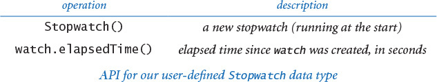
In other words, a Stopwatch object is a stripped-down version of an old-fashioned stopwatch. When you create one, it starts running, and you can ask it how long it has been running by invoking the method elapsedTime(). You might imagine adding all sorts of bells and whistles to Stopwatch, limited only by your imagination. Do you want to be able to reset the stopwatch? Start and stop it? Include a lap timer? These sorts of things are easy to add (see EXERCISE 3.2.11).
The implementation in stopwatch.py takes advantage of the Python function time() in the time module, which returns a float giving the current time in seconds (typically, the number of seconds since midnight on January 1, 1970 UTC). The data-type implementation could hardly be simpler. A Stopwatch object saves its creation time in an instance variable, then returns the difference between that time and the current time whenever a client calls its elapsedTime() method. A Stopwatch object itself does not actually tick (an internal system clock on your computer does all the ticking for all Stopwatch objects); it just creates the illusion that it does for clients. Why not just use time.time() in clients? We could do so, but using the higher-level Stopwatch abstraction leads to client code that is easier to understand and maintain.
The test client is typical. It creates two Stopwatch objects, uses them to measure the running time of two different computations and then writes the ratio of the running times.
The question of whether one approach to solving a problem is better than another has been lurking since the first few programs that you have run, and plays an essential role in program development. In SECTION 4.1, we will develop a scientific approach to understanding the cost of computation. Stopwatch is a useful tool in that approach.
Program 3.2.2 Stopwatch (stopwatch.py)
import math
import sys
import time
import stdio
class Stopwatch:
def __init__(self):
self._start = time.time()
def elapsedTime(self):
return time.time() - self._start
def main():
n = int(sys.argv[1])
total1 = 0.0
watch1 = Stopwatch()
for i in range(1, n+1):
total1 += i**2
time1 = watch1.elapsedTime()
total2 = 0.0
watch2 = Stopwatch()
for i in range(1, n+1):
total2 += i*i
time2 = watch2.elapsedTime()
stdio.writeln(total1/total2)
stdio.writeln(time1/time2)
if __name__ == '__main__': main()
instance variable
_start | creation time
This module defines a class Stopwatch that implements a data type that we can use to compare running times of performance-critical methods (see SECTION 4.1). The test client accepts an integer n from the command line and compares the cost for squaring a number using either i**2 or i*i for the task of computing the sum of the squares of the numbers from 1 to n. This quick test indicates that i*i is about three times faster than i**2.
% python stopwatch.py 1000000
1.0
3.179422835633626
Histogram
PROGRAM 3.2.3 (histogram.py) defines a data type Histogram for graphically representing the distribution of data using bars of different heights in a chart known as a histogram. A Histogram object maintains an array of the frequency of occurrence of integer values in a given interval. It uses stdstats.plotBars() to display a histogram of the values, controlled by this API:

With this simple data type, we reap the benefits of modular programming (reusable code, independent development of small programs, and so forth) that we discussed in CHAPTER 2, with the additional benefit that we also separate the data. A histogram client need not maintain the data (or know anything about its representation); it just creates a histogram and calls addDataPoint().
When studying this code and the next several examples, it is best to carefully consider the client code. Each class that we implement essentially extends the Python language, allowing us to create objects of the new data type and perform operations on them. All client programs are conceptually the same as the first programs that you learned that use built-in data types. Now you have the ability to define whatever types and operations you need in your client code!
In this case, using Histogram actually enhances the readability of the client code, as the addDataPoint() call focuses attention on the data being studied. Without Histogram, we would have to mix the code for creating the histogram with the code for the computation of interest, resulting in a program that is much more difficult to understand and maintain than the two separate programs. Whenever you can clearly separate data and associated operations within a computation, you should do so.
Once you understand how a data type will be used in client code, you can consider the implementation. An implementation is characterized by its instance variables (data-type values). Histogram maintains an array with the frequency of each point. Its draw() method scales the drawing (so that the tallest bar fits snugly in the canvas) and then plots the frequencies.
Program 3.2.3 Histogram (histogram.py)
import sys
import stdarray
import stddraw
import stdrandom
import stdstats
class Histogram:
def __init__(self, n):
self._freq = stdarray.create1D(n, 0)
def addDataPoint(self, i):
self._freq[i] += 1
def draw(self):
stddraw.setYscale(0, max(self._freq))
stdstats.plotBars(self._freq)
def main():
n = int(sys.argv[1])
p = float(sys.argv[2])
trials = int(sys.argv[3])
histogram = Histogram(n+1)
for t in range(trials):
heads = bernoulli.binomial(n, p)
histogram.addDataPoint(heads)
stddraw.setCanvasSize(500, 200)
histogram.draw()
stddraw.show()
if __name__ == '__main__': main()
instance variables
_freq[] | frequency counts

This module defines a Histogram class that implements a data type for creating dynamic histograms. The frequency counts are kept in an instance-variable array _freq. The test client accepts integer n, float p, and integer trials as command-line arguments. It performs trials experiments, each of which counts the number of heads found when a biased coin (heads with probability p and tails with probability 1 - p) is flipped n times. Then, it draws the results to standard drawing.
Turtle graphics
Whenever you can clearly separate tasks within a computation, you should do so. In object-oriented programming, we extend that mantra to include state with the tasks. A small amount of state can be immensely valuable in simplifying a computation. Next, we consider turtle graphics, which is based on the data type defined by this API:

Imagine a turtle that lives in the unit square and draws lines as it moves. It can move a specified distance in a straight line, or it can rotate left (counterclockwise) a specified number of degrees. According to the API, when we create a turtle, we place it at a specified point, facing a specified direction. Then, we create drawings by giving the turtle a sequence of goForward() and turnLeft() commands.
For example, to draw a triangle we create a turtle at (0, 0.5) facing at an angle of 60 degrees counterclockwise from the x-axis, then direct it to take a step forward, then rotate 120 degrees counterclockwise, then take another step forward, then rotate another 120 degrees counterclockwise, and then take a third step forward to complete the triangle. Indeed, all of the turtle clients that we will examine simply create a turtle, then give it an alternating series of step and rotate commands, varying the step size and the amount of rotation. As you will see in the next several pages, this simple model allows us to create arbitrarily complex drawings, with many important applications.
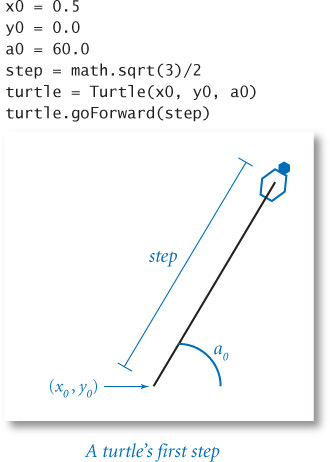
The Turtle class defined in PROGRAM 3.2.4 (turtle.py) is an implementation of this API that uses stddraw. It maintains three instance variables: the coordinates of the turtle’s position and the current direction it is facing, measured in degrees counterclockwise from the x-axis (polar angle). Implementing the two methods requires updating the values of these variables, so Turtle objects are mutable. The necessary updates are straightforward: turnLeft(delta) adds delta to the current angle, and goForward(step) adds the step size times the cosine of its argument to the current x-coordinate and the step size times the sine of its argument to the current y-coordinate.

The test client in Turtle takes an integer n as a command-line argument and draws a regular polygon with n sides. If you are interested in elementary analytic geometry, you might enjoy verifying that fact. Whether or not you choose to do so, think about what you would need to do to compute the coordinates of all the points in the polygon. The simplicity of the turtle’s approach is very appealing. In short, turtle graphics serves as a useful abstraction for describing geometric shapes of all sorts. For example, we obtain a good approximation to a circle by taking n to a sufficiently large value.

You can use a Turtle as you use any other object. Programs can create arrays of Turtle objects, pass them as arguments to functions, and so forth. Our examples will illustrate these capabilities and convince you that creating a data type like Turtle is both very easy and very useful. For each of them, as with regular polygons, it is possible to compute the coordinates of all the points and draw straight lines to get the drawings, but it is easier to do so with a Turtle. Turtle graphics exemplifies the value of data abstraction.
Program 3.2.4 Turtle graphics (turtle.py)
import math
import sys
import stddraw
class Turtle:
def __init__(self, x0, y0, a0):
self._x = x0
self._y = y0
self._angle = a0
def turnLeft(self, delta):
self._angle += delta
def goForward(self, step):
oldx = self._x
oldy = self._y
self._x += step * math.cos(math.radians(self._angle))
self._y += step * math.sin(math.radians(self._angle))
stddraw.line(oldx, oldy, self._x, self._y)
def main():
n = int(sys.argv[1])
step = math.sin(math.radians(180.0/n))
turtle = Turtle(.5, .0, 180.0/n)
for i in range(n):
turtle.goForward(step)
turtle.turnLeft(360.0/n)
stddraw.show()
if __name__ == '__main__': main()
instance variables
_x, _y | position (in unit square)
_angle | polar angle (in degrees)
This data type supports turtle graphics, which often simplifies the creation of drawings.


Recursive graphics
A Koch curve of order 0 is a straight line. To form a Koch curve of order n, draw a Koch curve of order n − 1, turn left 60 degrees, draw a second Koch curve of order n − 1, turn right 120 degrees (left −120 degrees), draw a third Koch curve of order n − 1, turn left 60 degrees, and draw a fourth Koch curve of order n − 1. These recursive instructions lead immediately to turtle client code. With appropriate modifications, recursive schemes like this have proved useful in modeling self-similar patterns found in nature, such as snowflakes.
The client code below is straightforward, except for the value of the step size. If you carefully examine the first few examples, you will see (and be able to prove by induction) that the width of the curve of order n is 3n times the step size, so setting the step size to 1/3n produces a curve of width 1. Similarly, the number of steps in a curve of order n is 4n, so koch.py will not finish if you invoke it for large n.
You can find many examples of recursive patterns of this sort that have been studied and developed by mathematicians, scientists, and artists from many cultures in many contexts. Here, our interest in them is that the turtle graphics abstraction greatly simplifies the client code that draws them.
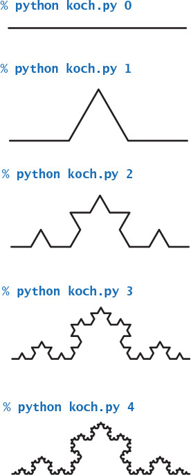
import sys
import stddraw
from turtle import Turtle
def koch(n, step, turtle):
if n == 0:
turtle.goForward(step)
return
koch(n-1, step, turtle)
turtle.turnLeft(60.0)
koch(n-1, step, turtle)
turtle.turnLeft(-120.0)
koch(n-1, step, turtle)
turtle.turnLeft(60.0)
koch(n-1, step, turtle)
n = int(sys.argv[1])
stddraw.setPenRadius(0.0)
step = 3.0 ** -n
turtle = Turtle(0.0, 0.0, 0.0)
koch(n, step, turtle)
stddraw.show()
Drawing Koch curves with turtle graphics
Spira mirabilis
Perhaps the turtle is a bit tired after taking 4n steps to draw a Koch curve (or just lazy). Accordingly, imagine that the turtle’s step size decays by a tiny constant factor (close to 1) each time it takes a step. What happens to our drawings? Remarkably, modifying the polygon-drawing test client in PROGRAM 3.2.4 to answer this question leads to an image known as a logarithmic spiral, a curve that is found in many contexts in nature.
PROGRAM 3.2.5 (spiral.py) is an implementation of this curve. It instructs the turtle to alternately step and turn until it has wound around itself a given number of times, with the step size decaying by a constant factor after each step. The script takes three command-line arguments, which control the shape and nature of the spiral. As you can see from the four examples given with the program, the path spirals into the center of the drawing. You are encouraged to experiment with spiral.py yourself to develop an understanding of the way in which the parameters control the behavior of the spiral.
The logarithmic spiral was first described by René Descartes in 1638. Jacob Bernoulli was so amazed by its mathematical properties that he named it the spira mirabilis (miraculous spiral) and even asked to have it engraved on his tombstone. Many people also consider it to be “miraculous” that this precise curve is clearly present in a broad variety of natural phenomena. Three examples are depicted below: the chambers of a nautilus shell, the arms of a spiral galaxy, and the cloud formation in a tropical storm. Scientists have also observed it as the path followed by a hawk approaching its prey and the path followed by a charged particle moving perpendicular to a uniform magnetic field.
One of the goals of scientific enquiry is to provide simple but accurate models of complex natural phenomena. Our tired turtle certainly passes that test!

Program 3.2.5 Spira mirabilis (spiral.py)
import math
import sys
import stddraw
from turtle import Turtle
n = int(sys.argv[1])
wraps = int(sys.argv[2])
decay = float(sys.argv[3])
angle = 360.0 / n
step = math.sin(math.radians(angle/2.0))
turtle = Turtle(0.5, 0, angle/2.0)
stddraw.setPenRadius(0)
for i in range(wraps * n):
step /= decay
turtle.goForward(step)
turtle.turnLeft(angle)
stddraw.show()
n | number of sides
wraps | wrap count
step | step size
decay | decay factor
angle | rotation amount
step | step size
turtle | lazy turtle
This code is a modification of the test client in PROGRAM 3.2.4 that decreases the step size at each step and cycles around a given number of times. The value of n controls the shape; wraps controls its extent; and decay controls the nature of the spiral.


Brownian motion
Or perhaps the turtle has had one too many. Accordingly, imagine that the disoriented turtle (again following its standard alternating turn-and-step regimen) turns in a random direction before each step. Again, it is easy to plot the path followed by such a turtle for millions of steps, and again, such paths are found in nature in many contexts. In 1827, the botanist Robert Brown observed through a microscope that tiny particles ejected from pollen grains seemed to move about in just such a random fashion when immersed in water. This process later became known as Brownian motion and led to Albert Einstein’s insights into the atomic nature of matter.
Or perhaps our turtle has friends, all of whom have had one too many. After they have wandered around for a sufficiently long time, their paths merge together and become indistinguishable from a single path. Astrophysicists today are using this model to understand observed properties of distant galaxies.
Turtle graphics was originally developed by Seymour Papert at MIT in the 1960s as part of an educational programming language, Logo, that is still used today in toys. But turtle graphics is no toy, as we have just seen in numerous scientific examples. Turtle graphics also has numerous commercial applications. For example, it is the basis for PostScript, a programming language for creating printed pages that is used for most newspapers, magazines, and books. In the present context, Turtle is a quintessential object-oriented programming example, showing that a small amount of saved state (data abstraction using objects, not just functions) can vastly simplify a computation.
import sys
import stddraw
import stdrandom
from turtle import Turtle
trials = int(sys.argv[1])
step = float(sys.argv[2])
stddraw.setPenRadius(0.0)
turtle = Turtle(0.5, 0.5, 0.0)
for t in range(trials):
angle = stdrandom.uniformFloat(0.0, 360.0)
turtle.turnLeft(angle)
turtle.goForward(step)
stddraw.show(0)
stddraw.show()

import sys
import stdarray
import stddraw
import stdrandom
from turtle import Turtle
n = int(sys.argv[1])
trials = int(sys.argv[2])
step = float(sys.argv[3])
stddraw.setPenRadius(0.0)
turtles = stdarray.create1D(n)
for i in range(n):
x = stdrandom.uniformFloat(0.0, 1.0)
y = stdrandom.uniformFloat(0.0, 1.0)
turtles[i] = Turtle(x, y, 0.0)
for t in range(trials):
for i in range(n):
angle = stdrandom.uniformFloat(0.0, 360.0)
turtles[i].turnLeft(angle)
turtles[i].goForward(step)
stddraw.show(0)
stddraw.show()

Complex numbers
A complex number is a number of the form x + yi, where x and y are real numbers and i is the square root of –1. The number x is known as the real part of the complex number, and the number y is known as the imaginary part. This terminology stems from the idea that the square root of –1 has to be an imaginary number, because no real number can have this value. Complex numbers are a quintessential mathematical abstraction: whether or not one believes that it makes sense physically to take the square root of –1, complex numbers help us understand the natural world. They are used extensively in applied mathematics and play an essential role in many branches of science and engineering. They are used to model physical systems of all sorts, from circuits to sound waves to electromagnetic fields. These models typically require extensive computations involving manipulating complex numbers according to well-defined arithmetic operations, so we want to compose computer programs to do the computations. In short, we need a new data type.
No programming language can provide implementations of every mathematical abstraction that we might possibly need, but the ability to implement data types give us not just the ability to compose programs to easily manipulate abstractions such as complex numbers, polynomials, vectors, and matrices, but also the freedom to think in terms of new abstractions.
The Python language provides a complex (with a lowercase c) data type. However, since developing a data type for complex numbers is a prototypical exercise in object-oriented programming, we now consider our own Complex (with an uppercase C) data type. Doing so will allow us to consider a number of interesting issues surrounding data types for mathematical abstractions, in a nontrivial setting.
The operations on complex numbers that are needed for basic computations are to add and multiply them by applying the commutative, associative, and distributive laws of algebra (along with the identity i2 = –1); to compute the magnitude; and to extract the real and imaginary parts, according to the following equations:
• Addition: (x+yi) + (v+wi) = (x+v) + (y+w)i
• Multiplication: (x + yi) * (v + wi) = (xv – yw) + (yv + xw) i
• Magnitude: ![]()
• Real part: Re(x + yi) = x
• Imaginary part: Im(x + yi) = y
For example, if a = 3 + 4i and b = –2 + 3i, then a +b = 1 + 7i, a *b = –18 + i, Re(a) = 3, Im(a) = 4, and |a| = 5.
With these basic definitions, the path to implementing a data type for complex numbers is clear. As usual, we start with an API that specifies the data-type operations. For simplicity, we concentrate in the text on just the basic operations in this API, but EXERCISE 3.2.18 asks you to consider several other useful operations that might be supported. Except for the uppercase C, this API is also implemented by Python’s built-in data type complex.

Special methods
How can we implement data-type operations so that clients can invoke them using arithmetic operators, such as + and *? The answer is found in another set of Python special methods that are specifically designed for this purpose. For example, when Python sees the expression a + b in client code, it replaces it with the method call a.__add__(b). Similarly, Python replaces a * b with the method call a.__mul__(b). Therefore, we need only to implement the special methods __add__() and __mul__() for addition and multiplication to operate as expected. The mechanism is the same one that we used to support Python’s built-in str() function for Charge, by implementing the __str__() special method, except that the special methods for arithmetic operators take two arguments. The above API includes an extra column that maps the client operations to the special methods. We generally omit this column in our APIs because these names are standard, and irrelevant to clients. The list of Python special methods is extensive—we will discuss them further in SECTION 3.3.
Complex (PROGRAM 3.2.6) is a class that implements this API. It has all of the same components as did Charge (and every Python data-type implementation): instance variables (_re and _im), a constructor, methods, and a test client. The test client first sets z0 to 1 + i, then sets z to z0, and then evaluates the expressions:
z = z2 + z0 = (1 + i)2 + (1 + i) = (1 + 2i –1) + (1 + i) = 1 + 3i
z = z2 + z0 = (1 + 3i)2 + (1 + i) = (1 + 6i – 9) + (1 + i) = –7 + 7i
This code is straightforward and similar to code that you have seen earlier in this chapter.
Accessing instance variables in objects of this type
The implementations of both __add__() and __mul__() need to access values in two objects: the object passed as an argument and the object used to call the method (that is, the object referenced by self). When the client calls a.__add__(b), the parameter variable self is set to reference the same object as argument a does, and the parameter variable other is set to reference the same object as argument b does. We can access the instance variables of a using self._re and self._im, as usual. To access the instance variables of b, we use the code other._re and other._im. Since our convention is to keep the instance variables private, we do not access directly instance variables in another class. Accessing instance variables within another object in the same class does not violate this privacy policy.
Immutability
The two instance variables in Complex are set for each Complex object when it is created and do not change during the lifetime of an object. That is, Complex objects are immutable. We discuss the benefits of this design decision in SECTION 3.3.
Complex numbers are the basis for sophisticated calculations from applied mathematics that have many applications. Our main reason for developing Complex—even though complex is built-in to Python—is to demonstrate the use of Python’s special functions in a simple but authentic setting. In real applications, you certainly should take advantage of complex unless you find yourself wanting more operations than Python provides.
To give you a feeling for the nature of calculations involving complex numbers and the utility of the complex number abstraction, we next consider a famous example of a complex (or Complex) client.
Program 3.2.6 Complex numbers (complex.py)
import math
import stdio
class Complex:
def __init__(self, re=0, im=0):
self._re = re
self._im = im
def re(self): return self._re
def im(self): return self._im
def __add__(self, other):
re = self._re + other._re
im = self._im + other._im
return Complex(re, im)
def __mul__(self, other):
re = self._re * other._re - self._im * other._im
im = self._re * other._im + self._im * other._re
return Complex(re, im)
def __abs__(self):
return math.sqrt(self._re*self._re + self._im*self._im)
def __str__(self):
return str(self._re) + ' + ' + str(self._im) + 'i'
def main():
z0 = Complex(1.0, 1.0)
z = z0
z = z*z + z0
z = z*z + z0
stdio.writeln(z)
if __name__ == '__main__': main()
instance variables
_re | real part
_im | imaginary part
This data type enables us to compose Python programs that manipulate complex numbers.
% python complex.py
-7.0 + 7.0i
Mandelbrot set
The Mandelbrot set is a specific set of complex numbers discovered by Benoît Mandelbrot that has many fascinating properties. It is a fractal pattern that is related to the Barnsley fern, the Sierpinski triangle, the Brownian bridge, the Koch curve, the drunken turtle, and other recursive (self-similar) patterns and programs that we have seen in this book. Patterns of this kind are found in natural phenomena of all sorts, and these models and programs are very important in modern science.
The set of points in the Mandelbrot set cannot be described by a single mathematical equation. Instead, it is defined by an algorithm and, therefore, a perfect candidate for a complex client: we study the set by composing a program to plot it.
The rule for determining whether a complex number z0 is in the Mandelbrot set is deceptively simple. Consider the sequence of complex numbers z0, z1, z2, . . ., zt, . . ., where zt+1 = (zt)2 + z0. For example, this table shows the first few entries in the sequence corresponding to z0 =1 + i:

Now, if the sequence |zt| diverges to infinity, then z0 is not in the Mandelbrot set; if the sequence is bounded, then z0 is in the Mandelbrot set. For many points, the test is simple. For many other points, the test requires more computation, as indicated by the examples in this table:

For brevity, the numbers in the rightmost two columns of this table are given to just two decimal places. In some cases, we can prove whether numbers are in the set; for example, 0 + 0i is certainly in the set (since the magnitude of all the numbers in its sequence is 0), and 2 + 0i is certainly not in the set (since its sequence dominates the powers of 2, which diverge). In other cases, the growth is readily apparent; for example, 1 + i does not seem to be in the set. Other sequences exhibit a periodic behavior; for example, the sequence for 0 + i alternates between –1 + i and –i. And some sequences go on for a very long time before the magnitude of the numbers begins to get large.
To visualize the Mandelbrot set, we sample complex points, just as we sample real-valued points to plot a real-valued function. Each complex number x + yi corresponds to a point (x, y) in the plane, so we can plot the results as follows: for a specified resolution n, we define a regularly spaced n-by-n pixel grid within a specified square and draw a black pixel if the corresponding point is in the Mandelbrot set and a white pixel if it is not. This plot is a strange and wondrous pattern, with all the black dots connected and falling roughly within the 2-by-2 square centered at the point –1/2 + 0i. Large values of n produce higher-resolution images, albeit at the cost of more computation. Looking closer reveals self-similarities throughout the plot, as shown in the example at right. For example, the same bulbous pattern with self-similar appendages appears all around the contour of the main black cardioid region, of sizes that resemble the simple ruler function of PROGRAM 1.2.1. When we zoom in near the edge of the cardioid, tiny self-similar cardioids appear!

But how, precisely, do we produce such plots? Actually, no one knows for sure, because there is no simple test that enables us to conclude that a point is surely in the set. Given a complex point, we can compute the terms at the beginning of its sequence, but may not be able to know for sure that the sequence remains bounded. There is a simple mathematical test that tells us for sure that a point is not in the set: if the magnitude of any number in the sequence ever exceeds 2 (such as 1 + 3i), then the sequence surely will diverge.
PROGRAM 3.2.7 (mandelbrot.py) uses this test to plot a visual representation of the Mandelbrot set. Since our knowledge of the set is not quite black-and-white, we use grayscale in our visual representation. The basis of the computation is the function mandel(), which takes a complex argument z0 and an integer argument limit and computes the Mandelbrot iteration sequence starting at z0, returning the number of iterations for which the magnitude stays less than (or equal to) 2, up to the given limit.
For each pixel, the main script in mandelbrot.py computes the point z0 corresponding to the pixel and then computes 255 - mandel(z0, 255) to create a grayscale color for the pixel. Any pixel that is not black corresponds to a point that we know to be not in the Mandelbrot set because the magnitude of the numbers in its sequence exceeds 2 (and therefore will go to infinity). The black pixels (grayscale value 0) correspond to points that we assume to be in the set because the magnitude stayed less than (or equal to) 2 for 255 iterations, but we do not necessarily know for sure.
The complexity of the images that this simple program produces is remarkable, even when we zoom in on a tiny portion of the plane. For even more dramatic pictures, we can use color (see EXERCISE 3.2.32). Moreover, the Mandelbrot set is derived from iterating just one function (z2 + z0); we have a great deal to learn from studying the properties of other functions as well.
The simplicity of the code masks a substantial amount of computation. There are about 250,000 pixels in a 512-by-512 image, and all of the black ones require 255 iterations, so producing an image with mandelbrot.py requires hundreds of millions of operations on complex values. Accordingly, we use Python’s complex data type, which is certain to be more efficient than the Complex data type that we just considered (see EXERCISE 3.2.14).

Fascinating as it is to study, our primary interest in the Mandelbrot set is to illustrate that computing with a type of data that is a pure abstraction is a natural and useful programming activity. The client code in mandelbrot.py is a simple and natural expression of the computation, made so by the ease of designing, implementing, and using data types in Python.
Program 3.2.7 Mandelbrot set (mandelbrot.py)
import sys
import stddraw
from color import Color
from picture import Picture
def mandel(z0, limit):
z = z0
for i in range(limit):
if abs(z) > 2.0: return i
z = z*z + z0
return limit
n = int(sys.argv[1])
xc = float(sys.argv[2])
yc = float(sys.argv[3])
size = float(sys.argv[4])
pic = Picture(n, n)
for col in range(n):
for row in range(n):
x0 = xc - size/2 + size*col/n
y0 = yc - size/2 + size*row/n
z0 = complex(x0, y0)
gray = 255 - mandel(z0, 255)
color = Color(gray, gray, gray)
pic.set(col, n-1-row, color)
stddraw.setCanvasSize(n, n)
stddraw.picture(pic)
stddraw.show()
x0, y0 | point in square
z0 | x0 + y0 i
limit | iteration limit
xc, yc | center of square
size | square is size-by-size
n | grid is n-by-n pixels
pic | image for output
color | pixel color for output

This program takes three command-line arguments that specify the n-by-n grid and the center (xc, yc) and size of a square region of interest, and makes a digital image showing the result of sampling the Mandelbrot set in that region at a n-by-n grid of equally spaced pixels. It colors each pixel with a grayscale value that is determined by counting the number of iterations before the Mandelbrot sequence for the corresponding complex number exceeds 2.0, up to 255.
Commercial data processing
One of the driving forces behind the development of object-oriented programming has been the need for an extensive amount of reliable software for commercial data processing. As an illustration, we consider next an example of a data type that might be used by a financial institution to keep track of customer information.
Suppose that a stock broker needs to maintain customer accounts containing shares of various stocks. That is, the set of values the broker needs to process includes the customer’s name, number of different stocks held, number of shares and ticker symbol for each stock, and cash on hand. To process an account, the broker needs at least the operations defined in this API:

The broker certainly needs to buy, sell, and provide reports to the customer, but the first key to understanding this kind of data processing is to consider the StockAccount() constructor and the write() method in this API. The customer information has a long lifetime and needs to be saved in a file or database. To process an account, a client program needs to read information from the corresponding file; process the information as appropriate; and, if the information changes, write it back to the file, saving it for later. To enable this kind of processing, we need a file format and an internal representation, or a data structure, for the account information. The situation is analogous to what we saw for matrix processing in CHAPTER 1, where we defined a file format (numbers of rows and columns followed by the elements in row-major order) and an internal representation (Python two-dimensional arrays) to enable us to compose programs for the random surfer and other applications.
As a (whimsical) running example, we imagine that a broker is maintaining a small portfolio of stocks in leading software companies for Alan Turing, the father of computing. As an aside: Turing’s life story is a fascinating one that is worth investigating further. Among many other things, he worked on computational cryptography that helped to bring about the end of World War II, he developed the basis for modern theoretical computer science, he designed and built one of the first computers, and he was a pioneer in artificial intelligence research. It is perhaps safe to assume that Turing, whatever his financial situation as an academic researcher in the middle of the last century, would be sufficiently optimistic about the potential impact of computing software in today’s world that he would make some small investments.
File format
Modern systems often use text files, even for data, to minimize dependence on formats defined by any one program. For simplicity, we use a direct representation where we list the account holder’s name (a string), cash balance (a float), and number of stocks held (an integer), followed by a line for each stock giving the number of shares and the ticker symbol, as shown in the example at right. It is also wise to use tags such as <Name> and <Number of shares> and so forth to label all the information, to further minimize dependencies on any one program, but we omit such tags here for brevity.
% more turing.txt
Turing, Alan
10.24
4
100 ADBE
25 GOOG
97 IBM
250 MSFT
Data structure
To represent information for processing by Python programs, we define a data type and use instance variables to organize the information. The instance variables specify the type of information and provide the structure that we need to refer to it in code. For example, to implement a StockAccount, we use the following instance variables:
• A string for the account name
• A float for the cash on hand
• An integer for the number of stocks
• An array of strings for stock symbols
• An array of integers for numbers of shares
We directly reflect these choices in the instance variable declarations in StockAccount, defined in PROGRAM 3.2.8. The arrays _stocks[] and _shares[] are known as parallel arrays. Given an index i, _stocks[i] gives a stock symbol and _shares[i] gives the number of shares of that stock in the account. An alternative design would be to define a separate data type for stocks to manipulate this information for each stock and maintain an array of objects of that type in StockAccount.
StockAccount includes a constructor, which reads a file and builds an account with this internal representation. It also includes a method valueOf(), which uses stockquote.py (PROGRAM 3.1.10) to get each stock’s price from the web. To provide a periodic detailed report to customers, our broker might use the following code for writeReport() in StockAccount:
def writeReport(self):
stdio.writeln(self._name)
total = self._cash
for i in range(self._n):
amount = self._shares[i]
price = stockquote.priceOf(self._stocks[i])
total += amount * price
stdio.writef('%4d %4s ', amount, self._stocks[i])
stdio.writef(' %7.2f %9.2f
', price, amount*price)
stdio.writef('%21s %10.2f
', 'Cash:', self._cash)
stdio.writef('%21s %10.2f
', 'Total:', total)
On the one hand, this client illustrates the kind of computing that was one of the primary drivers in the evolution of computing in the 1950s. Banks and other companies bought early computers precisely because of the need to do such financial reporting. For example, formatted writing was developed precisely for such applications. On the other hand, this client exemplifies modern web-centric computing, as it gets information directly from the web, without using a browser.
The implementations of buy() and sell() require the use of basic mechanisms introduced in SECTION 4.4, so we defer them to EXERCISE 4.4.39. Beyond these basic methods, an actual application of these ideas would likely use a number of other clients. For example, a broker might want to create an array of all accounts, then process a list of transactions that both modify the information in those accounts and actually carry out the transactions through the web. Of course, such code needs to be developed with great care!
Program 3.2.8 Stock account (stockaccount.py)
import sys
import stdarray
import stdio
import stockquote
from instream import InStream
class StockAccount:
def __init__(self, filename):
instream = InStream(filename)
self._name = instream.readLine()
self._cash = instream.readFloat()
self._n = instream.readInt()
self._shares = stdarray.create1D(self._n, 0)
self._stocks = stdarray.create1D(self._n, 0)
for i in range(self._n):
self._shares[i] = instream.readInt()
self._stocks[i] = instream.readString()
def valueOf(self):
total = self._cash
for i in range(self._n):
price = stockquote.priceOf(self._stocks[i])
amount = self._shares[i]
total += amount * price
return total
def main():
acct = StockAccount(sys.argv[1])
acct.writeReport()
if __name__ == '__main__': main()
instance variables
_name | customer name
_cash | cash balance
_n | number of stocks
_shares[] | numbers of shares
_stocks[] | stock symbols
instream | input stream
% python stockaccount.py turing.txt
Turing, Alan
100 ADBE 70.56 7056.00
25 GOOG 502.30 12557.50
97 IBM 156.54 15184.38
250 MSFT 45.68 11420.00
Cash: 10.24
Total: 46228.12
This class for processing accounts illustrates typical usage of object-oriented programming for commercial data processing. See the text for the writeReport() method; see EXERCISE 3.2.20 for the write() method and EXERCISE 4.4.39 for the buy() and sell() methods.
When you learned how to define functions that can be used in multiple places in a program (or in other programs) in CHAPTER 2, you moved from a world where programs are simply sequences of statements in a single file to the world of modular programming, summarized in our mantra: whenever you can clearly separate tasks within a computation, you should do so. The analogous capability for data, introduced in this chapter, moves you from a world where data has to be one of a few elementary types of data to a world where you can define your own types of data. This profound new capability vastly extends the scope of your programming. As with the concept of a function, once you have learned to implement and use data types, you will marvel at the primitive nature of programs that do not use them.
But object-oriented programming is much more than structuring data. It enables us to associate the data relevant to a subtask with the operations that manipulate this data and to keep both separate in an independent module. With object-oriented programming, our mantra is this: whenever you can clearly separate data and associated operations within a computation, you should do so.
The examples that we have considered are persuasive evidence that object-oriented programming can play a useful role in a broad range of programming activities. Whether we are trying to design and build a physical artifact, develop a software system, understand the natural world, or process information, a key first step is to define an appropriate abstraction, such as a geometric description of the physical artifact, a modular design of the software system, a mathematical model of the natural world, or a data structure for the information. When we want to compose programs to manipulate instances of a well-defined abstraction, we implement the abstraction as a data type in a Python class and compose Python programs to create and manipulate objects of that type.
Each time that we develop a class that makes use of other classes by creating and manipulating objects of the type defined by the class, we are programming at a higher layer of abstraction. In the next section, we discuss some of the design challenges inherent in this kind of programming.