Chapter One. Elements of Programming
Our goal in this chapter is to convince you that composing a program is easier than writing a piece of text, such as a paragraph or essay. Writing prose is difficult: you spend many years in school to learn how to do it. By contrast, just a few building blocks suffice to enable you to compose programs that can solve all sorts of fascinating, but otherwise unapproachable, problems. In this chapter, we take you through these building blocks, get you started on programming in Python, and study a variety of interesting programs. You will be able to express yourself (by composing programs) within just a few weeks. Like the ability to write prose, the ability to program is a lifetime skill that you can continually refine well into the future.
In this book, you will learn the Python programming language. This task will be much easier for you than, for example, learning a foreign language. Indeed, programming languages are characterized by only a few dozen vocabulary words and rules of grammar. Much of the material that we cover in this book could also be expressed in the Java or C++ languages, or any of several other modern programming languages. We describe everything specifically in Python so that you can get started creating and running programs right away. On the one hand, we will focus on learning to program, as opposed to learning details about Python. On the other hand, part of the challenge of programming is knowing which details are relevant in a given situation. Python is widely used, so learning Python will enable you to compose programs on many computers (your own, for example). Also, learning to program in Python will make it easy for you to learn other languages, including lower-level languages such as C and specialized languages such as Matlab.
1.1 Your First Program
In this section, our plan is to lead you into the world of Python programming by taking you through the basic steps required to get a simple program running. The Python system (hereafter abbreviated Python) is a collection of applications, not unlike many of the other applications that you are accustomed to using (such as your word processor, email program, and web browser). As with any application, you need to be sure that Python is properly installed on your computer. It comes preloaded on many computers, or you can download it easily. You also need a text editor and a terminal application. Your first task is to find the instructions for installing such a Python programming environment on your computer by visiting
http://introcs.cs.princeton.edu/python
We refer to this site as the booksite. It contains an extensive amount of supplementary information about the material in this book for your reference and use while programming.
Programming in Python
To introduce you to developing Python programs, we break the process down into two steps. To program in Python, you need to:
• Compose a program by typing it into a file named, say, myprogram.py.
• Run (or execute) it by typing python myprogram.py in the terminal window.
In the first step, you start with a blank screen and end with a sequence of typed characters on the screen, just as when you write an email message or an essay. Programmers use the term code to refer to program text and the term coding to refer to the act of creating and editing the code. In the second step, you transfer control of the computer from the system to your program (which returns control back to the system when finished). Many systems support several different ways to compose and execute programs. We choose the sequence given here because it is the simplest to describe and use for small programs.
Composing a program
A Python program is nothing more than a sequence of characters, like a paragraph or a poem, stored in a file whose name has a .py extension. To compose one, therefore, you need simply define that sequence of characters, in the same way as you do for email or any other computer application. You can use any text editor for this task, or you can use one of the more sophisticated program development environments described on the booksite. Such environments are overkill for the sorts of programs we consider in this book, but they are not difficult to use, have many useful features, and are widely used by professionals.
Executing a program
Once you compose the program, you can run (or execute) it. This is the exciting part, where your program takes control of your computer (within the constraints of what Python allows). It is perhaps more accurate to say that your computer follows your instructions. It is even more accurate to say that the Python compiler translates your Python program into a language that is more suitable for execution on a computer. Then, the Python interpreter directs your computer to follow these instructions. Throughout this book we use the term executing or running to refer to the combination of compiling and interpreting a program (as in “When Python executes this program...”). To use the Python compiler and interpreter to execute your program, type the python command followed by the name of the file containing the Python program in a terminal window.
PROGRAM 1.1.1 is an example of a complete Python program. Its code resides in a file named helloworld.py. The program’s sole action is to write a message back to the terminal window. A Python program consists of statements. Typically you place each statement on a distinct line.
• The first line of helloworld.py contains an import statement. That statement tells Python that you intend to use the features defined in the stdio module—that is, in a file named stdio.py. The stdio.py file is one that we designed specifically for this book. It defines functions related to reading input and writing output. Having imported the stdio module, you can later call a function that is defined in that module.

Program 1.1.1 Hello, World (helloworld.py)
import stdio
# Write 'Hello, World' to standard output.
stdio.writeln('Hello, World')
This code is a Python program that accomplishes a simple task. It is traditionally a beginner’s first program. The box below shows what happens when you execute the program. The terminal application gives a command prompt (% in this book) and executes the commands that you type (in boldface in this book). The result of executing python with this code is that the program writes Hello, World in the terminal window (the fourth line).
% python helloworld.py
Hello, World
• The second line is a blank line. Python ignores blank lines; programmers use them to separate logical blocks of code.
• The third line contains a comment, which serves to document the program. In Python a comment begins with the ‘#’ character and extends to the end of the line. In this book, we display comments in gray. Python ignores comments—they are present only for human readers of the program.
• The fourth line is the heart of the program. It is a statement that calls the stdio.writeln() function to write one line with the given text on it. Note that we call a function in another module by writing the module name, followed by a period, followed by the function name.
Python 2
The lingua france in this book is Python 3, because it is the future of Python programming. However, we have been very careful to ensure that the code in the book works with either Python 2 or Python 3. For example, in Python 2, PROGRAM 1.1.1 could be simply the single line print 'Hello, World', but this is not a valid program in Python 3. To develop code for writing output that works in either version of Python, we use our stdio module. Whenever there is a significant difference between the two languages, we call attention to Python 2 users in a callout box like this one.
Since the 1970s, it has been a tradition that a beginning programmer’s first program should write 'Hello, World'. So, you should go ahead and type the code in PROGRAM 1.1.1 into a file named helloworld.py and then execute it. By doing so, you will be following in the footsteps of countless others who have learned how to program. Also, you will be checking that you have a usable editor and terminal application. At first, accomplishing the task of writing something out in a terminal window might not seem very interesting; upon reflection, however, you will see that one of the most basic functions that we need from a program is its ability to tell us what it is doing.
For the time being, all our program code will be just like helloworld.py, except with a different file name, different comments, and a different sequence of statements following the comment. Thus, you do not need to start with a blank page to compose a program. Instead,
• Copy helloworld.py into a new file having a name of your choice, but make sure that the new file name ends with .py.
• Replace the comment and the stdio.writeln() statement with a different sequence of statements.
Your program is characterized by its sequence of statements and its name. By convention, each Python program resides in a file whose name has a .py extension.
Errors
It is easy to blur the distinction among editing, compiling, and interpreting programs. You should keep them separate in your mind when you are learning to program, to better understand the effects of the errors that inevitably arise. You can find several examples of errors in the Q&A at the end of this section.
You can fix or avoid most errors by carefully examining the program as you create it, the same way you fix spelling and grammatical errors when you compose an email message. Some errors, known as compile-time errors, are raised when Python compiles the program, because they prevent the compiler from doing the translation. Python reports a compile-time error as a SyntaxError. Other errors, known as run-time errors, are not raised until Python interprets the program. For example, if you forget the import stdio statement in helloworld.py, then Python will raise a NameError at run time.
In general, errors in programs, also commonly known as bugs, are the bane of a programmer’s existence: the error messages can be confusing or misleading, and the source of the error can be very hard to find. One of the first skills that you will learn is to identify errors; you will also learn to be sufficiently careful when coding, to avoid making many of them in the first place.
Input and output
Typically, we want to provide input to our programs—that is, data that they can process to produce a result. The simplest way to provide input data is illustrated in useargument.py (PROGRAM 1.1.2). Whenever you run the program useargument.py, it accepts the command-line argument that you type after the program name and writes it back out to the terminal as part of the message. The result of executing this program depends on what you type after the program name. You can run the program with different command-line arguments and get different written results.
In useargument.py, the statement import sys tells Python that you wish to use the features defined in the sys module. One of those features, named argv, is a list of command-line arguments (which appear after “python useargument.py” on the command line, delimited by spaces). Later in the book (SECTION 2.1) we will discuss this mechanism in more detail. For now it is sufficient to understand that sys.argv[1] is the first command-line argument that you type after the program name, sys.argv[2] is the second command-line argument that you type after the program name, and so forth. You can use sys.argv[1] within your program’s body to represent the string that you type on the command line when you execute it, just as in useargument.py.

In addition to writeln(), PROGRAM 1.1.2 calls the write() function. This function is just like writeln(), but writes just the string (not a newline character).
Again, accomplishing the task of getting a program to write back out what we type in to it may not seem interesting at first, but upon reflection you will realize that another basic function of a program is its ability to respond to basic information from the user to control what the program does. The simple model that useargument.py represents will suffice to allow us to consider Python’s basic programming mechanism and to address all sorts of interesting computational problems.
Stepping back, we can see that useargument.py does neither more nor less than map a string of characters (the argument) into another string of characters (the message written back to the terminal). When using it, we might think of our Python program as a black box that converts our input string to some output string.
Program 1.1.2 Using a command-line argument (useargument.py)
import sys
import stdio
stdio.write('Hi, ')
stdio.write(sys.argv[1])
stdio.writeln('. How are you?')
This program shows how we can control the actions of our programs: by providing an argument on the command line. Doing so allows us to tailor the behavior of our programs. The program accepts a command-line argument, and writes a message that uses it.
% python useargument.py Alice
Hi, Alice. How are you?
% python useargument.py Bob
Hi, Bob. How are you?
% python useargument.py Carol
Hi, Carol. How are you?
This model is attractive because it is not only simple but also sufficiently general to allow completion, in principle, of any computational task. For example, the Python compiler itself is nothing more than a program that takes one string as input (a .py file) and produces another string as output (the corresponding program in a more primitive language). Later, you will be able to compose programs that accomplish a variety of interesting tasks (though we stop short of programs as complicated as a compiler). For the moment, we live with various limitations on the size and type of the input and output to our programs; in SECTION 1.5, you will see how to incorporate more sophisticated mechanisms for program input and output. In particular, you will see that we can work with arbitrarily long input and output strings and other types of data such as sound and pictures.
A. The programs that we are studying are very similar to their counterparts in several other languages, so our choice of language is not crucial. We use Python because it is widely available, embraces a full set of modern abstractions, and has a variety of automatic checks for mistakes in programs, so it is suitable for learning to program. Python is evolving and comes in many versions.
Q. Which version of Python should I use?
A. We recommend Python 3, but we have been very careful to ensure that the code in the book works with either Python 2 or Python 3. All of the code has been tested with Python versions 2.7 and 3.4 (the latest major releases of Python 2 and Python 3 at the time of publication). We use the generic term Python 2 to refer to Python 2.7 and Python 3 to refer to Python 3.4.
Q. How do I install a Python programming environment?
A. The booksite provides step-by-step instructions for installing a Python programming environment on your Mac OS X, Windows, or Linux system. This includes installation of our booksite modules, such as stdio.py.
Q. Do I really have to type in the programs in the book to try them out? I believe that you ran them and that they produce the indicated output.
A. You should type in and run helloworld.py. Your understanding will be greatly magnified if you also run useargument.py, try it on various inputs, and modify it to test different ideas of your own. To save some typing, you can find all of the code in this book (and much more) on the booksite. This site also has information about installing Python on your computer, answers to selected exercises, web links, and other extra information that you may find useful or interesting.
Q. When I run helloworld.py, Python generates the message
ImportError: No module named stdio.
What does that mean?
A. That means that the booksite module stdio is not available to Python.
Q. How can I make the booksite module stdio available to Python?
A. If you followed the step-by-step instructions on the booksite for installing a Python programming environment, the stdio module should already be available to Python. Alternatively, you can download the file stdio.py from the booksite and put it in the same directory as the program that uses it.
Q. What are Python’s rules regarding whitespace characters such as tabs, spaces, and newlines?
A. In general, Python considers most whitespace in program text to be equivalent, with two important exceptions: string literals and indentation. A string literal is a sequence of characters inside single quotes, such as 'Hello, World'. If you put any number of spaces within the quotes, you get precisely the same number of spaces in the string literal. Indentation is whitespace at a beginning of a line—the number of spaces at the beginning of a line plays an important role in structuring Python programs, as we will see in SECTION 1.3. For now you should not indent any code.
Q. Why should I use comments?
A. Comments are indispensable because they help other programmers to understand your code and even can help you to understand your own code in retrospect. The constraints of the book format demand that we use comments sparingly in the programs shown in this book (instead we describe each program thoroughly in the accompanying text and figures). The programs on the booksite are commented to a more realistic degree.
Q. Can I put more than one statement on a line?
A. Yes, by separating statements with semicolons. For example, this single line of code produces the same output as helloworld.py:
import stdio; stdio.writeln('Hello, World')
But many programmers advise against doing this, as a matter of style.
Q. What happens when you omit a parenthesis or misspell one of the words, like stdio or write or writeln?
A. It depends upon precisely what you do. These so-called syntax errors are usually caught by the compiler. For example, if you make a program bad.py that is exactly the same as helloworld.py except that you omit the first left parenthesis, you get the following reasonably helpful message:
% python bad.py
File "bad.py", line 4
stdio.write'Hello, World')
∧
SyntaxError: invalid syntax
From this message, you might correctly surmise that you need to insert a left parenthesis. But the compiler may not be able to tell you exactly which mistake you made, so the error message may be hard to understand. For example, if you omit the first right parenthesis instead of the first left parenthesis, you get the following less helpful message, which references the line following the erroneous one:
% python bad.py
File "bad.py", line 5
^
SyntaxError: unexpected EOF while parsing
One way to get used to such messages is to intentionally introduce mistakes into a simple program and then see what happens. Whatever the error message says, you should treat the compiler as a friend, because it is just trying to tell you that something is wrong with your program.
Q. When I run useargument.py, I get a strange error message. Please explain.
A. Most likely, you forgot to include a command-line argument:
% python useargument.py
Hi, Traceback (most recent call last):
File "useargument.py", line 5, in <module>
stdio.write(sys.argv[1])
IndexError: list index out of range
The Python interpreter is complaining that you ran the program but did not type a command-line argument as promised. You will learn more details about list indices in SECTION 1.4. Remember this error message: you are likely to see it again. Even experienced programmers forget to type command-line arguments on occasion.
Q. Which Python modules and functions are available for me to use?
A. Many standard modules are bundled with any Python installation. Many others are available as extension modules that you can download and install subsequently. We composed still others (such as the stdio module) specifically for this book and booksite; we’ll call them booksite modules. In short, hundreds of Python modules, each (typically) defining multiple functions, are available for you to use. This book introduces only the most fundamental modules and functions, and does so in a deliberately incremental fashion (starting in the next section) to avoid overwhelming you with information.
1.1.2 Describe what happens if you omit the following in helloworld.py:
a. import
b. stdio
c. import stdio
1.1.3 Describe what happens if you misspell (by, say, omitting the second letter) the following in helloworld.py:
a. import
b. stdio
c. write
d. writeln
1.1.4 Describe what happens if you omit the following in helloworld.py:
a. the first '
b. the second '
c. the stdio.writeln() statement
1.1.5 Describe what happens if you try to execute useargument.py with each of the following command lines:
a. python useargument.py python
b. python useargument.py @!&∧%
c. python useargument.py 1234
d. python useargument Bob
e. useargument.py Bob
f. python useargument.py Alice Bob
1.1.6 Modify useargument.py to compose a program usethree.py that takes three names and writes a proper sentence with the names in the reverse of the order they are given, so that, for example, python usethree.py Alice Bob Carol writes the string 'Hi Carol, Bob, and Alice'.
1.2 Built-in Types of Data
When programming in Python, you must always be aware of the type of data that your program is processing. The programs in SECTION 1.1 process strings, many of the programs in this section process numbers, and we consider numerous other types later in the book. Understanding the distinctions among them is so important that we formally define the idea: a data type is a set of values and a set of operations defined on those values.
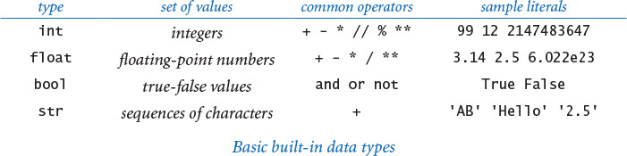
Several data types are built into the Python language. In this section, we consider Python’s built-in data types int (for integers), float (for floating-point numbers), str (for sequences of characters) and bool (for true-false values), which are summarized in the table below.
For now, we concentrate on programs that are based on computing with these four basic built-in data types. Later, you will learn about additional data types that are available for your use, and you will learn how to compose your own data types. Indeed, programming in Python often is centered on composing data types, as you will see in CHAPTER 3.
After defining basic terms, we consider several sample programs and code fragments that illustrate the use of different types of data. These code fragments do not perform much real computing, but you will soon see similar code in longer programs. Understanding data types (values and operations on them) is an essential step in beginning to program. It sets the stage for you to begin working with more intricate programs in the next section. Every program that you compose will use code like the tiny fragments shown in this section.
Definitions
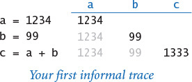
To talk about data types, we need to introduce some terminology. To do so, we start with the following code fragment:
a = 1234
b = 99
c = a + b
This code creates three objects, each of type int, using the literals 1234 and 99 and the expression a + b, and binds (“bind” is a technical term indicating the creation of an association) variables a, b, and c to those objects using assignment statements. The end result is that variable c is bound to an object of type int whose value is 1333. Next, we define all of these italicized terms.
Literals
A literal is a Python-code representation of a data-type value. We use sequences of digits such as 1234 or 99 to represent values of data type int; we add a decimal point, as in 3.14159 or 2.71828, to represent values of type float, we use True or False to represent the two values of type bool; and we use a sequence of characters enclosed in matching quotes, such as 'Hello, World', to represent values of type str.
Operators
An operator is a Python-code representation of a data-type operation. Python uses + and * to represent addition and multiplication for integers and floating-point numbers; Python uses and, or, and not to represent boolean operations; and so forth. We will describe in detail the most commonly used operations for each of the four basic built-in types later in this section.
Identifiers
An identifier is a Python-code representation of a name. Each identifier is a sequence of letters, digits, and underscores, the first of which is not a digit. The sequences of characters abc, Ab_, abc123, and a_b are all legal Python identifiers, but Ab*, 1abc, and a+b are not. Identifiers are case-sensitive, so Ab, ab, and AB are all different names. Certain keywords—such as and, import, in, def, while, from, and lambda—are reserved, and you cannot use them as identifiers. Other names—such as int, sum, min, max, len, id, file, and input—have special meaning in Python, so it is best not to use them, either.
Variables
A variable is a name associated with a data-type value. We use variables to keep track of changing values as a computation unfolds. For example, we use a variable total in several programs in this book to keep the running total of a sum of a sequence of numbers. Programmers typically follow stylistic conventions when naming things. In this book our convention is to give each variable a name that consists of a lowercase letter followed by lowercase letters, uppercase letters, and digits. We use uppercase letters to mark the words of a multi-word variable name. So, for example, we use the variable names i, x, y, total, isLeapYear, and outDegrees, among many others.
Constant variables
We use the oxymoronic term constant variable to describe a variable whose associated a data-type value does not change during the execution of a program (or from one execution of the program to the next). In this book, our convention is to give each constant variable a name that consists of an uppercase letter followed by uppercase letters, digits, and underscores. For example, we might use the constant variable names SPEED_OF_LIGHT and DARK_RED.
Expressions
An expression is a combination of literals, variables, and operators that Python evaluates to produce a value. Many expressions look just like mathematical formulas, using operators to specify data-type operations to be performed on one or more operands. Most of the operators that we use are binary operators that take exactly two operands, such as x - 3 or 5 * x. Each operand can be any expression, perhaps within parentheses. For example, we can compose expressions like 4 * (x - 3) or 5 * x - 6 and Python will understand what we mean. An expression is a directive to perform a sequence of operations; the expression is a representation of the resulting value.

Operator precedence
An expression is shorthand for a sequence of operations: in which order should the operators be applied? Python has natural and well-defined precedence rules that fully specify this order. For arithmetic operations, multiplication and division are performed before addition and subtraction, so that a - b * c and a - (b * c) represent the same sequence of operations. When arithmetic operators have the same precedence, they are left associative, which means that a - b - c and (a - b) - c represent the same sequence of operations. The exponentiation operator ** is the exception: it is right associative, which means that a ** b ** c and a ** (b ** c) represent the same sequence of operations. You can use parentheses to override the rules, so you can write a - (b - c) if that is what you want. You might encounter in the future some Python code that depends subtly on precedence rules, but we use parentheses to avoid such code in this book. If you are interested, you can find full details on the rules on the booksite.
Assignment statements
How do we define an identifier to be a variable in Python code? How do we associate a variable with a data-type value? In Python, we use an assignment statement for both purposes. When we write a = 1234 in Python, we are not expressing mathematical equality, but are instead expressing an action, directing Python to
• define the identifier a to be a new variable (if no variable a already exists).
• associate the variable a with the integer data-type value 1234.
The right side of an assignment statement can be any expression. In such cases, Python evaluates the expression and associates the variable on the left side with the value produced by the expression. For example, when we write c = a + b, we are expressing this action: “associate the variable c with the sum of the values associated with the variables a and b.” The left side of an assignment statement must be a single variable. So, for example, both 1234 = a and a + b = b + a are invalid statements in Python. In short, the meaning of = in a program is decidedly not the same as in a mathematical equation.
Informal trace
An effective way to keep track of the values associated with variables is to use a table like the one at right, with one line giving the values after each statement has been executed. Such a table is called a trace, and is a time-honored technique for understanding the behavior of a program. We use traces like this throughout this book.
While descriptions of this sort are a valid way to understand the Python code in this section, it is worthwhile at the outset to consider in more detail how Python represents data-type values using objects and to revisit the definitions in that context. While these definitions are more complicated than the ones just considered, it is important for you to understand the underlying mechanism, as it is used consistently throughout Python and prepares you for object-oriented programming in CHAPTER 3.
Objects
All data values in a Python program are represented by objects and relationships among objects. An object is an in-computer-memory representation of a value from a particular data type. Each object is characterized by its identity, type, and value.
• The identity uniquely identifies an object. You should think of it as the location in the computer’s memory (or memory address) where the object is stored.
• The type of an object completely specifies its behavior—the set of values it might represent and the set of operations that can be performed on it.
• The value of an object is the data-type value that it represents.
Each object stores one value; for example, an object of type int can store the value 1234 or the value 99 or the value 1333. Different objects may store the same value. For example, one object of type str might store the value 'hello', and another object of type str also might store the same value 'hello'. We can apply to an object any of the operations defined by its type (and only those operations). For example, we can multiply two int objects but not two str objects.
Object references
An object reference is nothing more than a concrete representation of the object’s identity (the memory address where the object is stored). Python programs use object references either to access the object’s value or to manipulate the object references themselves, as you will see.
Formal object-based definitions
Now, we consider more formal definitions for the terminology we have been using.

• A literal is a directive to Python to create an object having the specified value.
• A variable is a name for an object reference. We use diagrams like the one at right to show the binding of a variable to an object.
• An expression is a directive to Python to perform the indicated operations, producing an object having the value defined by the expression.
• An assignment statement is a directive to Python to bind the variable on the left side of the = operator to the object produced by evaluating the expression on the right side (regardless of the object, if any, to which the variable was previously bound).
Object-level trace
For a more complete understanding, we sometimes keep track of objects and references in traces, as in the object-level trace in the figure at right. For our example, the object-level trace illustrates the full effect of the three assignment statements:
• The statement a = 1234 creates an int object whose value is 1234; it then binds the variable a to this new int object.
• The statement b = 99 creates an int object whose value is 99; it then binds the variable b to this new int object.
• The statement c = a + b creates the int object whose value is 1333 as the sum of the value of the int object bound to a and the value of the int object bound to b; it then binds the variable c to the new int object.
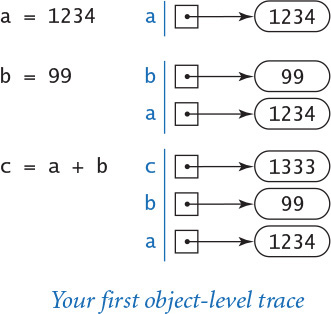
Throughout this book, we generally use the more succinct and intuitive informal traces just discussed, reserving object-level traces for situations when they provide a more insightful view of the underlying computation.
Example: incrementing a variable
As a first check on these concepts, consider the following code, which binds the variable i to an int object whose value is 17, and then increments it:
i = 17
i = i + 1
As we have noted, this second statement is nonsensical as a mathematical equality, but it is a very common operation in Python programming. Specifically, these two statements are a directive to Python to take the following actions:
• Create an int object whose value is 17 and bind the variable i to that object.
• Evaluate the expression i + 1 and create a new int object whose value is 18.
• Bind the variable i to this new object.
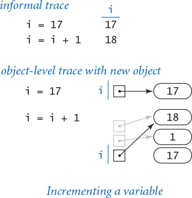
You can consult the traces at right to see the results after Python executes each statement.
This simple code fragment leads us to consider two aspects of the process of creating an object in a bit more detail. First, the assignment statement i = i + 1 does not change the value of any object. Instead, it creates a new object (with the desired value) and binds the variable i to this new object. Second, after Python executes the assignment statement i = i + 1, there is no variable bound to the object whose value is 17 (or to the object whose value is 1). Python takes responsibility for managing memory resources. When it identifies that a program can no longer access an object, it automatically reclaims the memory used to store the object.
Example: exchanging two variables
As a second check on these concepts, convince yourself that this code exchanges a and b (more precisely, the objects bound to a and b):
t = a
a = b
b = t
To do so, assume that a and b are bound to objects having two different values—1234 and 99, respectively—and consult the traces at right to convince yourself, step by step, that:
• t = a assigns a to t. That is, it assigns a (an object reference) to t, and thus a and t are bound to the same object—the int object whose value is 1234.
• a = b assigns b to a. That is, it assigns b (an object reference) to a, and thus a and b are bound to the same object—the int object whose value is 99.
• b = t assigns t to b. That is, it assigns t (an object reference) to b, and thus t and b are bound to the same object—the int object whose value is 1234.

Thus, the references are exchanged: the variable a now is bound to the object whose value is 99 and the variable b now is bound to the object whose value is 1234.
You might wonder whether the distinction between an object and a reference to an object is purely pedantic. In fact, understanding the difference between objects and references is the key to mastering many important features of Python programming, including functions (in CHAPTER 2), object-oriented programming (in CHAPTER 3), and data structures (in CHAPTER 4).
Next, we consider the details for the data types that you will use most often (strings, integers, floating-point numbers, and boolean values), along with sample code illustrating their use. To use a data type, you need to know not just its set of values, but also which operations you can perform, the language mechanism for invoking the operations, and the conventions for specifying literals.
Strings
The str data type represents strings, for use in text processing. The value of a str object is a sequence of characters. You can specify a str literal by enclosing a sequence of characters in matching single quotes; for example 'ab', represents a str object that stores two characters, the letter 'a' followed by the letter 'b'. There are many possible characters, but we usually restrict attention to the ones that represent letters, digits, symbols, and whitespace characters such as tab and newline. You can use a backslash to specify characters that otherwise would have special meaning. For example, you can specify the tab, newline, backslash, and single quote characters using the escape sequences ' ', '
', '', and ''', respectively.

You can concatenate two strings using the operator +. That is, the + operator takes two str objects as operands and produces a new str object whose value is the sequence of characters in the first str object followed by the sequence of characters in the second str object. For example, the expression '123' + '456' evaluates to the str object whose value is '123456'. This example illustrates that applying the + operator to two str objects has quite different behavior (string concatenation) than applying the + operator to two int objects (addition).

Program 1.2.1 String concatenation example (ruler.py)
import stdio
ruler1 = '1'
ruler2 = ruler1 + ' 2 ' + ruler1
ruler3 = ruler2 + ' 3 ' + ruler2
ruler4 = ruler3 + ' 4 ' + ruler3
stdio.writeln(ruler1)
stdio.writeln(ruler2)
stdio.writeln(ruler3)
stdio.writeln(ruler4)
% python ruler.py
1
1 2 1
1 2 1 3 1 2 1
1 2 1 3 1 2 1 4 1 2 1 3 1 2 1
This program writes the relative lengths of the subdivisions on a ruler. The nth line of output is the relative lengths of the marks on a ruler subdivided in intervals of 1/2n of an inch.
String concatenation is sufficiently powerful to allow us to attack some nontrivial computing tasks. As an example, ruler.py (PROGRAM 1.2.1) computes a table of values of the ruler function that describes the relative lengths of the marks on a ruler. One noteworthy feature of this computation is that it illustrates how easy it is to craft short programs that produce huge amounts of output. If you extend this program in the obvious way to write five lines, six lines, seven lines, and so forth, you will see that each time you add just two statements to this program, you increase the size of its output by precisely one more than a factor of 2. Specifically, if the program writes n lines, the nth line contains 2n – 1 numbers. For example, if you were to add statements in this way so that the program writes 30 lines, it would attempt to write more than 1 billion numbers.

Next we consider two convenient mechanisms in Python for converting numbers to strings and strings to numbers.
Converting numbers to strings for output
Python provides the built-in function str() to convert numbers to strings. For example, str(123) evaluates to the str object '123', and str(123.45) evaluates to the str object '123.45'. If the argument to either stdio.write() or stdio.writeln() is not of type str, then these two functions automatically call the str() function on its argument to generate the string representation. For example, stdio.write(123), stdio.write(str(123)), and stdio.write('123') all write 123.
Our most frequent use of the string concatenation operator is to chain together the results of a computation for output with stdio.write() and stdio.writeln(), often in conjunction with the str() function, as in this example:
stdio.writeln(str(a) + ' + ' + str(b) + ' = ' + str(a+b))
If a and b are int objects whose values are 1234 and 99, respectively, then that statement writes the line of output 1234 + 99 = 1333. We consider the str data type first precisely because we need it to produce this sort of output in programs that process other types of data.
Converting strings to numbers for input
Python also provides built-in functions to convert strings (such as the ones we type as command-line arguments) to numeric objects. We use the Python built-in functions int() and float() for this purpose. For example, typing int('1234') in program text is equivalent to typing the int literal 1234. If the user types 1234 as the first command-line argument, then the code int(sys.argv[1]) also evaluates to the int object whose value is 1234. You will see several examples of this usage in this section.
With these features, our view of each Python program as a black box that takes string arguments and produces string results is still valid, but we can now interpret those strings as numbers and use them as the basis for meaningful computation.

Integers
The int data type represents integers or natural numbers. We can specify an int literal with a sequence of the digits 0 through 9. When Python encounters an int literal, it creates an int object that stores the specified value. We use int objects frequently not just because they occur frequently in the real world, but also because they arise naturally when we are composing programs.
Python includes operators for common arithmetic operations on integers, including + for addition, - for subtraction, * for multiplication, // for floored division, % for remainder, and ** for exponentiation. These binary operators take two int objects as operands and typically produce an int object as a result. Python also includes the unary operators + and - to specify the sign of an integer. All of these operators are defined just as in grade school (keeping in mind that the floored division operator results in an integer): given two int objects a and b, the expression a // b evaluates to the number of times b goes into a with the fractional part discarded, and a % b evaluates to the remainder that you get when you divide a by b. For example, 17 // 3 evaluates to 5, and 17 % 3 evaluates to 2. Floored division or remainder with a zero divisor raises a ZeroDivisionError at run time.

PROGRAM 1.2.2 (intops.py) illustrates basic operations for manipulating int objects, such as the use of expressions involving arithmetic operators. It also demonstrates the use of the built-in function int() to convert strings on the command line to int objects, as well as the use of the built-in function str() to convert int objects to strings for output.
Program 1.2.2 Integer operators (intops.py)
import sys
import stdio
a = int(sys.argv[1])
b = int(sys.argv[2])
total = a + b
diff = a - b
prod = a * b
quot = a // b
rem = a % b
exp = a ** b
stdio.writeln(str(a) + ' + ' + str(b) + ' = ' + str(total))
stdio.writeln(str(a) + ' - ' + str(b) + ' = ' + str(diff))
stdio.writeln(str(a) + ' * ' + str(b) + ' = ' + str(prod))
stdio.writeln(str(a) + ' // ' + str(b) + ' = ' + str(quot))
stdio.writeln(str(a) + ' % ' + str(b) + ' = ' + str(rem))
stdio.writeln(str(a) + ' ** ' + str(b) + ' = ' + str(exp))
This program accepts integer command-line arguments a and b, uses them to illustrate integer operators, and writes the results. Arithmetic for integers is built into Python. Most of this code is devoted to reading input and writing output; the actual arithmetic is in the simple statements in the middle of the program that assign values to total, diff, prod, quot, rem, and exp.
% python intops.py 1234 5
1234 + 5 = 1239
1234 - 5 = 1229
1234 * 5 = 6170
1234 // 5 = 246
1234 % 5 = 4
1234 ** 5 = 2861381721051424
In Python, the range of int values is arbitrarily large, constrained only by the amount of memory available on your computer system. Many other programming languages constrain the range of integers. For example, the Java programming language constrains integers to the range –231 (–2147483648) to 231 – 1 (2147483647). On the one hand, Python programmers do not have to worry about integers becoming too large to fit in the allowed range; on the other hand, Python programmers do have to worry about a faulty program filling the memory of their computer with one or more extremely huge integers.

Python 2 alert
In Python 3, the / operator has the same behavior as the floating-point division operator when both its operands are integers. In Python 2, the / operator has the same behavior as the floored division operator // when both its operands are integers. For example, 17 / 2 evaluates to 8.5 in Python 3 and to 8 in Python 2. For compatibility among Python versions, we do not use the / operator with two int operands in this book.
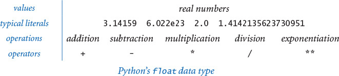
Floating-point numbers
The float data type is for representing floating-point numbers, for use in scientific and commercial applications. We use floating-point numbers to represent real numbers, but they are decidedly not the same as real numbers! There are infinitely many real numbers, but we can represent only a finite number of floating-point numbers in any digital computer. Floating-point numbers do approximate real numbers sufficiently well that we can use them in applications, but we often need to cope with the fact that we cannot always do exact computations.
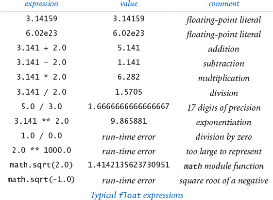
We can specify a floating-point literal using a sequence of digits with a decimal point. For example, 3.14159 represents an approximation to π. Alternatively, we can use a notation like scientific notation: the literal 6.022e23 represents the number 6.022 × 10²³. As with integers, you can use these conventions to express floating-point literals in your programs or to provide floating-point numbers as string arguments on the command line.
PROGRAM 1.2.3 (floatops.py) illustrates the basic operations for manipulating float objects. Python includes the operators you expect for floating-point numbers, including + for addition, - for subtraction, * for multiplication, / for division, and ** for exponentiation. These operators take two float objects as operands and typically produce a float object as a result. PROGRAM 1.2.3 also illustrates the use of the float() function to convert a str object to a float object, and the use of the str() function to convert a float object to a str object.
Program 1.2.3 Float operators (floatops.py)
import sys
import stdio
a = float(sys.argv[1])
b = float(sys.argv[2])
total = a + b
diff = a - b
prod = a * b
quot = a / b
exp = a ** b
stdio.writeln(str(a) + ' + ' + str(b) + ' = ' + str(total))
stdio.writeln(str(a) + ' - ' + str(b) + ' = ' + str(diff))
stdio.writeln(str(a) + ' * ' + str(b) + ' = ' + str(prod))
stdio.writeln(str(a) + ' / ' + str(b) + ' = ' + str(quot))
stdio.writeln(str(a) + ' ** ' + str(b) + ' = ' + str(exp))
This program takes floating-point numbers a and b as command-line arguments, uses them to illustrate floating-point operations, and writes the results. Arithmetic for floating-point numbers is built into Python. As with PROGRAM 1.2.2, most of this code is devoted to reading input and writing output; the actual arithmetic is in the simple statements in the middle of the program that assign values to total, diff, prod, quot, and exp.
% python floatops.py 123.456 78.9
123.456 + 78.9 = 202.356
123.456 - 78.9 = 44.556
123.456 * 78.9 = 9740.6784
123.456 / 78.9 = 1.5647148288973383
123.456 ** 78.9 = 1.0478827916671325e+165
When working with floating-point numbers, one of the first things that you will encounter is the issue of precision: 5.0/2.0 evaluates to 2.5 but 5.0/3.0 evaluates to 1.6666666666666667. Typically, floating-point numbers have 15-17 decimal digits of precision. In SECTION 1.5, you will learn Python’s mechanism for controlling the number of digits that you see in output. Until then, we will work with Python’s default output format. Though there are myriad details to consider when calculations involve float objects, you can use them in a natural way and compose Python programs instead of using a calculator for all kinds of calculations. For example, quadratic.py (PROGRAM 1.2.4) shows the use of float objects in computing the two roots of a quadratic equation using the quadratic formula.
Note the use of the math.sqrt() function in this program. The standard math module defines trigonometric functions, logarithm/exponential functions, and other common mathematical functions. When Python calls the function, it produces a value—the value computed by the function. You can use the math module in the same way that we have been using stdio in every program since helloworld.py: place the statement import math near the beginning of the program and then call functions using syntax such as math.sqrt(x). We discuss in more detail the mechanism behind this arrangement in SECTION 2.1 and provide more details about the math module at the end of this section.
As illustrated in the sample execution accompanying PROGRAM 1.2.4, quadratic.py does not check for error conditions. In particular, it assumes that the roots are real numbers. If not, it calls math.sqrt() with a negative number as its argument, which raises a ValueError at run time. Generally, it is good programming practice to check for such errors and inform the user about them. We will discuss how to do so after you learn a few more Python language mechanisms.
Program 1.2.4 Quadratic formula (quadratic.py)
import math
import sys
import stdio
b = float(sys.argv[1])
c = float(sys.argv[2])
discriminant = b*b - 4.0*c
d = math.sqrt(discriminant)
stdio.writeln((-b + d) / 2.0)
stdio.writeln((-b - d) / 2.0)
This program writes the roots of the polynomial x2 + bx + c, using the quadratic formula. For example, the roots of x2 – 3x + 2 are 1 and 2 since we can factor the equation as (x – 1)(x – 2); the roots of x2 – x – 1 are ϕ and 1 – ϕ, where ϕ is the golden ratio, and the roots of x2 + x + 1 are not real numbers.
% python quadratic.py -3.0 2.0
2.0
1.0
% python quadratic.py -1.0 -1.0
1.618033988749895
-0.6180339887498949
% python quadratic.py 1.0 1.0
Traceback (most recent call last):
File "quadratic.py", line 9, in <module>
d = math.sqrt(discriminant)
ValueError: math domain error
Booleans
The bool data type represents truth values (either true or false) from logic. The data type has two possible values and two corresponding literals: True and False. The bool operations that we use have operands that are either True or False and evaluate to a result that is also either True or False. This simplicity is deceiving—the bool data type lies at the foundation of computer science. The operators defined for bool objects (and, or, and not) are known as logical operators and have familiar definitions:
• a and b is True if both operands are True, and False if either is False.
• a or b is False if both operands are False, and True if either is True.
• not a is True if a is False, and False if a is True.
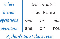
Despite the intuitive nature of these definitions, it is worthwhile to fully specify each possibility for each operation in truth tables, as shown at the bottom of this page. The not operator has only one operand: its result for each of the two possible values of the operand is specified in the second column. The and and or operators each have two operands: the results for each of the four possible values of these operands are specified in the right two columns.
We can use these operators with parentheses (and precedence rules) to develop arbitrarily complex expressions, each of which specifies a boolean function. The not operator has higher precedence than the and operator, which in turn has higher precedence than the or operator.
Often the same function appears in different guises. For example, the expressions (a and b) and not (not a or not b) are equivalent. One way to establish that this is the case is to use a truth-table proof like the one at the top of the next page, which checks all possibilities.

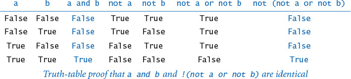
The study of manipulating expressions of this kind is known as Boolean logic. This field of mathematics is fundamental to computing: it plays an essential role in the design and operation of computer hardware itself, and it is also a starting point for the theoretical foundations of computation. In the present context, we are interested in bool expressions because we use them to control the behavior of our programs. Typically, a particular condition of interest is specified as a boolean expression and a piece of program code is written to execute one set of statements if the expression evaluates to True and a different set of statements if the expression evaluates to False. The mechanics of doing so are the topic of SECTION 1.3.
Comparisons
Some mixed-type operators take operands of one type and produce a result of another type. The most important operators of this kind are the comparison operators ==, !=, <, <=, >, and >=, which all are defined for both integers and floats and evaluate to a boolean result. Since operations are defined only with respect to data types, each of these operators stands for many operations, one for each data type. Both operands must be of compatible type. The result is always a boolean.


Even without going into the details of number representation, it is clear that the operations for the various types are really quite different. For example, it is one thing to compare two integers to check that (2 <= 2) is True, but quite another to compare two floats to check whether (2.0 <= 0.002e3) is True. Still, these operations are well defined and useful to compose code that tests for conditions such as (b*b - 4.0*a*c) >= 0.0, which is frequently needed, as you will see.
Comparison operators have lower precedence than arithmetic operators and higher precedence than boolean operators, so you do not need the parentheses in an expression like (b*b - 4.0*a*c) >= 0.0, and you could write an expression like month >= 1 and month <= 12 without parentheses to test whether month is between 1 and 12. (It is better style to use the parentheses, however.)
Comparison operations, together with boolean logic, provide the basis for decision making in Python programs. PROGRAM 1.2.5 (leapyear.py) shows the use of boolean expressions and comparison operations to compute whether a given year is a leap year. You can find other examples in the exercises at the end of this section. More importantly, in SECTION 1.3 we will see the role that boolean expressions play in more sophisticated programs.
PROGRAM 1.2.5 also illustrates a special and useful property of the logical operators known as short-circuiting: the and operator evaluates the second operand only if the first operand is True; the or operator evaluates the second operand only if the first operand is False. For example, in leapyear.py, Python evaluates the comparison expression (year % 100) != 0 only if the year is divisible by 4 and the comparison expression (year % 400) != 0 only if the year is divisible by 100.
Functions and APIs
As we have seen, many programming tasks involve using not only built-in operators, but also functions that perform useful operations. We distinguish three kinds of functions: built-in functions (such as int(), float(), and str()) that you can use directly in any Python program, standard functions (such as math.sqrt()) that are defined in a Python standard module and are available in any program that imports the module, and booksite functions (such as stdio.write() and stdio.writeln()) that are defined in our booksite modules and available for you to use after you have made them available to Python and imported them. The number of built-in functions, standard functions, and booksite functions available to you is very large. As you learn to program, you will learn to use more and more of those functions, but it is best at the beginning to restrict your attention to a relatively small set. In this chapter, you have already used some functions for writing, for converting data from one type to another, and for computing mathematical functions. We will describe some more useful functions in this section. In later chapters, you will learn not just how to use other functions, but how to define and use your own functions.
Program 1.2.5 Leap year (leapyear.py)
import sys
import stdio
year = int(sys.argv[1])
isLeapYear = (year % 4 == 0)
isLeapYear = isLeapYear and ((year % 100) != 0)
isLeapYear = isLeapYear or ((year % 400) == 0)
stdio.writeln(isLeapYear)
This program tests whether an integer corresponds to a leap year in the Gregorian calendar. A year is a leap year if it is divisible by 4 (2004), unless it is divisible by 100 in which case it is not (1900), unless it is divisible by 400 in which case it is (2000).
% python leapyear.py 2016
True
% python leapyear.py 1900
False
% python leapyear.py 2000
True
For convenience, we summarize the functions that you need to know how to use in tables like the one shown on the facing page. It includes examples of built-in functions, booksite functions from our stdio module, and standard functions from Python’s math and random modules. Such a table is known as an application programming interface (API). The first column specifies the information you need to use the function, including its name and its number of arguments; the second column describes its purpose.
In your code, you can call a function by typing its name followed by arguments, enclosed in parentheses and separated by commas. When Python executes your program, we say that it calls (or evaluates) the function with the given arguments and that the function returns a value. More precisely, the function returns a reference to an object, which has a value. A function call is an expression, so you can use a function call in the same way that you use variables and literals to build up more complicated expressions. For example, you can compose expressions like math.sin(x) * math.cos(y) and so on. You can also represent an argument using an expression—Python evaluates the expression and passes the result as an argument to the function. So, you can compose code like math.sqrt(b*b - 4.0*a*c) and Python knows what you mean.
In some cases, a function can have default values for optional arguments. The function math.log() is an example—it takes the base of the logarithm as an optional second argument, defaulting to the natural logarithm (base e) if you do not specify a second argument.
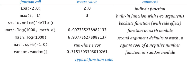
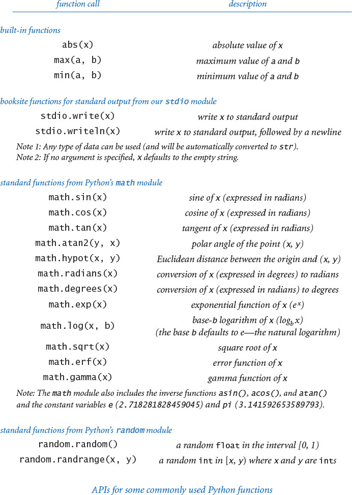
With three exceptions, the functions on the previous page are pure functions—given the same arguments, they always return the same value, without producing any observable side effect. The function random.random() is impure because it returns potentially a different value each time it is called; the functions stdio.write() and stdio.writeln() are impure because they produce side effects—writing strings to standard output. In APIs, we use a verb phrase to describe the behavior of a function that produces side effects; otherwise, we use a noun phrase to describe the return value.
The math module also defines the constant variables math.pi (for π) and math.e (for e), so that you can use those names to refer to those constants in your programs. For example, the function call math.sin(math.pi/2) returns 1.0 (because math.sin() takes its argument in radians) and the function call math.log(math.e) returns 1.0 (because the default base for math.log() is e).
These APIs are typical of the online documentation that is the standard in modern programming. There is extensive online documentation of the Python APIs that is used by professional programmers, and it is available to you (if you are interested) through our booksite. You do not need to consult the online documentation to understand the code in this book or to compose similar code, because we present and explain in the text all of the functions that we use in APIs like these and summarize them in the endpapers.
More important, in CHAPTERS 2 and 3 you will learn how to develop your own APIs and to implement functions for your own use.
Type conversion
Typical programming tasks involve processing multiple types of data. You should always be aware of the type of data that your program is processing, because only by knowing the type can you know precisely which set of values each object can have and which operations you can perform. In particular, we often need to convert data from one type to another. For example, suppose that we wish to compute the average of the four integers 1, 2, 3, and 4. Naturally, the expression (1 + 2 + 3 + 4) / 4 comes to mind, but it does not produce the desired result in many programming languages, because of type conversion conventions. Indeed, as we have already noted, Python 3 and Python 2 produce different results for this expression, so it is a worthy example for introducing this topic.
The problem stems from the fact that the operands are integers, but it is natural to expect a float for the result, so conversion from integer to float is necessary at some point. There are two ways to do so in Python.
Explicit type conversion
One approach is to use a function that takes an argument of one type (the object to be converted) and returns an object of another type. We have already used the built-in functions int(), float(), and str() to convert from strings to integers or floats, and vice versa. This is by far their most common usage, but you can also use them (and the additional function round()) to convert between integers and floats, as shown in the API at the top of the next page. For example, you can use either int(x) or int(round(x)) to convert from a float to an integer and float(x) to convert from an integer to a float. So, the expression float(1 + 2 + 3 + 4) / float(4) evaluates to 2.5 in both Python 3 and Python 2, as you would expect.
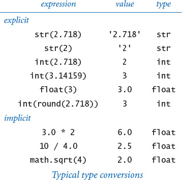
Python 2 alert
In Python 3, round(x) returns an integer; in Python 2, round(x) returns a float. In this book, we always use the expression int(round(x)) to round a float x to the nearest integer, so that the code works in both Python 3 and Python 2.

Implicit type conversion (from integer to float)
You can use an integer where a float is expected, because Python automatically converts integers to floats when appropriate. For example, 10/4.0 evaluates to 2.5 because 4.0 is a float and both operands need to be of the same type; thus, 10 is converted to a float and then the result of dividing two floats is a float. For another example, math.sqrt(4) evaluates to 2.0 because the 4 is converted to a float, as expected by math.sqrt(), which then returns a float. This kind of conversion is called automatic promotion or coercion. It is appropriate that Python implements automatic promotion because it can be done with no loss of information. But, as we have noted, there are pitfalls. For example, as we have seen, Python 3 automatically promotes each integer operand of the / operator to a float but Python 2 does not do so. So, (1 + 2 + 3 + 4) / 4 evaluates to the float 2.5 in Python 3 but to the integer 2 in Python 2.
The concept of automatic promotion is irrelevant if you always use the int() and float() functions to indicate your type-conversion wishes explicitly; in turn, some programmers avoid automatic promotion whenever possible. In this book we generally do rely upon automatic promotion because it leads to compact and easy-to-read code. However, whenever we want to divide two numbers with the / operator, we always arrange for (at least) one of the two operands to be a float. For our examples, when Python evaluates the expression (1 + 2 + 3 + 4) / 4.0, it triggers automatic promotion to a float for the first operand and produces the float 2.5, as expected. This practice ensures that our code works properly in both Python 3 and Python 2 (and many other languages). Again, in this book, we do not use the / operator when both operands are integers.
Beginning programmers tend to find type conversion to be an annoyance, but experienced programmers know that paying careful attention to data types is a key to success in programming. It may also be a key to avoiding failure: In a famous incident in 1985, a French rocket exploded in midair because of a type-conversion problem. While a bug in your program may not cause an explosion, it is well worth your while to take the time to understand what type conversion is all about. After you have written just a few programs, you will see that an understanding of data types will help you not only compose compact code but also make your intentions explicit and avoid subtle bugs in your programs.

Summary
A data type is a set of values and a set of operations defined on those values. Python has built-in data types bool, str, int, and float; you will encounter others later in this book. In Python code, we use operators and expressions like those in familiar mathematical expressions to invoke the operations associated with each type. The bool type is for computing with true-false values; the str type is for sequences of characters; the int and float data types are numeric types, for computing with numbers.
The bool type (which includes the logical operators and, or, and not) is the basis for logical decision making in Python programs, when used in conjunction with the comparison operators ==, !=, <, <=, >, and >=. Specifically, we use bool expressions to control Python’s conditional (if) and loop (while) statements, which we will study in detail in the next section.
The numeric types, built-in functions, and functions defined in Python’s standard and extension modules and in our booksite modules give us the ability to use Python as an extensive mathematical calculator. We compose arithmetic expressions using the built-in operators +, -, *, /, //, %, and ** along with Python function calls.
Although the programs in this section are rudimentary by the standards of what we will be able to do after the next section, this class of programs is quite useful in its own right. You will use data types and basic mathematical functions extensively in Python programming, so the effort that you spend now in understanding them certainly will be worthwhile.
Interactive Python
Indeed, we can use Python as a calculator, directly. To do that, issue the command python (that is, the word python stand-alone, with no following file name) in your terminal window. Python identifies itself, and writes a >>> prompt. At that point you can type a Python statement and Python will execute it. Or, you can type a Python expression and Python will evaluate it and write the resulting value. Or, you can type help() to get access to Python’s extensive interactive documentation. Some examples are shown below (boldface indicates what you type). This is a convenient way to test new constructs and access documentation, thereby learning about modules and functions that are of interest to you. You are encouraged to do so in several of the Q&A sections that follow.
% python
...
>>> 1 + 2
3
>>> a = 1
>>> b = 2
>>> a + b
3
>>> import math
>>> math.sqrt(2.0)
1.4142135623730951
>>> math.e
2.718281828459045
>>>
% python
...
>>> import math
>>> help(math)
Help on module math:
NAME
math
DESCRIPTION
This module is always available. It provides
access to the mathematical functions defined
by the C standard.
FUNCTIONS
acos(...)
acos(x)
Return the arc cosine (in radians) of x.
...
sqrt(...)
sqrt(x)
Return the square root of x
...
DATA
e = 2.718281828459045
pi = 3.141592653589793
Strings in Python 2
Python 2 uses ASCII instead of Unicode to encode characters. ASCII is a legacy standard that supports 128 characters, including the English alphabet, numbers, and punctuation. Python 2 offers a separate data type unicode for strings composed of Unicode characters, but many Python 2 libraries do not support it.
A. Strings are sequences of characters that are encoded with Unicode, a modern standard for encoding text. Unicode supports over 100,000 different characters, including more than 100 different languages plus mathematical and musical symbols.
Q. Which data type does Python provide for characters?
A. Python has no special data type for characters. A character is simply a string consisting of one element, such as 'A'.
Q. Can I compare strings using comparison operators such as == and < or built-in functions such as max() and min()?
A. Yes. Informally, Python uses lexicographic order to compare two strings, like words in a book index or dictionary. For example, 'hello' and 'hello' are equal, 'hello' and 'goodbye' are unequal, and 'goodbye' is less than 'hello'. See the Q&A at the end of SECTION 4.2 for full details.
Q. Can I use matching double quotes for string literals instead of single quotes?
A. Yes. For example, 'hello’ and "hello" are identical literals. Double quotes are useful to specify a string that contains single quotes, so that you don’t need to escape them. For example, 'Python's’ and "Python's" are identical string literals. You can also use matching triple quotes for multiline strings. For example, the following creates a two-line string and assigns it to the variable s:
s = """Python's "triple" quotes are useful to
specify string literals that span multiple lines
"""
In this book, we do not use double or triple quotes to delimit string literals.
A. The simplest representation is for small positive integers, where the binary number system is used to represent each integer with a fixed amount of computer memory.
Q. What’s the binary number system?
A. You probably learned it in grade school. In the binary number system, we represent an integer as a sequence of bits. A bit is a single binary (base 2) digit—either 0 or 1—and is the basis for representing information in computers. In this case the bits are coefficients of powers of 2. Specifically, the sequence of bits bnbn–1...b2b1b0 represents the integer
bn2n +bn–12n–1 +...b222 +b121 +b020
For example, 1100011 represents the integer
99 = 1· 64 + 1· 32 + 0· 16 + 0· 8 + 0· 4 + 1· 2 +1· 1.
The more familiar decimal number system is the same except that the digits are between zero and 9 and we use powers of 10. Converting a number to binary is an interesting computational problem that we will consider in the next section. For small integers, Python uses a fixed number of bits, typically dictated by a basic design parameter of your computer—usually 32 or 64. For example, the integer 99 might be represented with the 32 bits 00000000000000000000000001100011.
Q. How about negative numbers?
A. Small negative numbers are handled with a convention known as two’s complement, which we need not consider in detail. The definition of “small” depends on the underlying computer system. On older 32-bit machines, “small” typically covers the range –2147483648 (–231) to 2147483647 (231 – 1). On newer 64-bit machines, “small” typically covers the range –263 to 263 – 1, in which case “small” is not so small! If an integer is not “small,” then Python automatically uses a more elaborate representation whose range is limited only by the amount of memory available on your computer system. Note that details of these internal representations are hidden from your programs, so you can use them systems with different representations without having to change them.
Q. What does the expression 1/0 evaluate to in Python?
A. It raises a ZeroDivisionError at run time. Note: The easiest way to answer such questions is to use Python’s interactive mode. Try it!
Q. How do the floored division operator // and remainder operator % work on negative operands?
A. Try them and see! -47 // 5 evaluates to -10 and -47 % 5 evaluates to 3. Generalizing, the floored division operator // yields the floored quotient; that is, the quotient is rounded toward minus infinity. The behavior of the remainder operator % is more complicated. In Python, if a and b are integers, then the expression a % b evaluates to an integer that has the same sign as b. This implies that b * (a // b) + a % b == a for any integers a and b. In some other languages (such as Java), the expression a % b evaluates to an integer that has the same sign as a.
Q. How does the exponentiation operator ** work with negative operands?
A. Try it out and see for yourself. Note that the ** operator has higher precedence than a unary plus/minus operator on its left but lower precedence than a unary plus/minus operator on its right. For example, -3**4 evaluates to -81 (and not 81). Also, it can result in an object of a different type. For example, 10**-2 evaluates to the float 0.01 and (-10)**(10**-2) evaluates to a complex number in Python 3 (but raises a run-time error in Python 2).
Q. Why does 10∧6 evaluate to 12 instead of 1000000?
A. The ∧ operator is not an exponentiation operator, which you must have been thinking. Instead, it is an operator that we do not use in this book. You want the literal 1000000. You could use the expression 10**6, but it is wasteful to use an expression (which requires evaluation at run time) when a literal would suffice.
Integers in Python 2
Python 2 supports two separate types for integers—int (for small integers) and long (for larger integers). Python 2 automatically promotes from type int to long whenever necessary.
A. The decimal point can “float” across the digits that make up the real number. In contrast, with integers the (implicit) decimal point is fixed after the least significant digit.
Q. How does Python store floating-point numbers internally?
A. Generally, Python uses the representation that is natural for the underlying computer system. Most modern computer systems store floating-point numbers as defined by the IEEE 754 standard. That standard specifies that a floating-point number is stored using three fields: sign, mantissa, and exponent. If you are interested, see the booksite for more details. The IEEE 754 standard also specifies how special floating-point values—positive zero, negative zero, positive infinity, negative infinity, and NaN (not a number)—should be handled. For example, it specifies that -0.0/3.0 should evaluate to -0.0, 1.0/0.0 should evaluate to positive infinity, and 0.0/0.0 should evaluate to NaN. You can use the (rather unusual) expressions float('inf') and float('-inf') for positive and negative infinity in some simple calculations, but Python does not conform to this part of the IEEE 754 standard. For example, in Python, -0.0/3.0 correctly evaluates to -0.0, but both 1.0/0.0 and 0.0/0.0 raise a ZeroDivisionError at run time.
Q. Fifteen digits for floating-point numbers certainly seems enough to me. Do I really need to worry much about precision?
A. Yes, because you are used to mathematics based on real numbers with infinite precision, whereas the computer always deals with approximations. For example, in IEEE 754 floating point, the expression (0.1 + 0.1 == 0.2) evaluates to True but (0.1 + 0.1 + 0.1 == 0.3) evaluates to False! Pitfalls like this are not at all unusual in scientific computing. Novice programmers should avoid comparing two floating-point numbers for equality.
Q. It is annoying to see all those digits when writing a float. Is it possible to get stdio.write() and stdio.writeln() to write just two or three digits after the decimal point?
A. The booksite function stdio.writef() is one way to do the job—it is similar to the basic formatted writing function in the C programming language and many other modern languages, as discussed in SECTION 1.5. Until then, we will live with the extra digits (which is not all bad, since doing so helps us to get used to the different types of numbers).
Q. Can I apply the floored division operator // to two float operands?
A. Yes, it produces the floored division of its operands. That is, the result is the quotient in which digits after the decimal place are removed. We do not use the floored division operator on floats in this book.
Q. What does round() return if the fractional part of its argument is 0.5?
A. In Python 3, it returns the nearest even integer, so round(2.5) is 2, round(3.5) is 4, and round(-2.5) is -2. But in Python 2, the round() function rounds away from zero (and returns a float), so round(2.5) is 3.0, round(3.5) is 4.0, and round(-2.5) is -3.0.
Q. Can I compare a float to an int?
A. Not without doing a type conversion, but remember that Python does the requisite type conversion automatically. For example, if x is the integer 3, then the expression (x < 3.1) evaluates to True because Python promotes the integer 3 to generate the float 3.0 and then compares 3.0 with 3.1.
Q. Are there functions in Python’s math module for other trigonometric functions, such as arc sine, hyperbolic sine, and secant?
A. Yes, Python’s math module includes inverse trigonometric functions and hyperbolic functions. However, there are no functions for secant, cosecant, and cotangent because you could use math.sin(), math.cos(), and math.tan() to compute them easily. Choosing which functions to include in an API is a tradeoff between the convenience of having every function that you need and the annoyance of having to find one of the few that you need in a long list. No choice will satisfy all users, and the Python designers have many users to satisfy. Note that there are plenty of redundancies even in the APIs that we have listed. For example, you could use math.sin(x) / math.cos(x) instead of math.tan(x).
A. Python will raise a NameError at run time.
Q. How can I determine the type of a variable?
A. That’s a trick question. Unlike variables in many programming languages (such as Java), a Python variable does not have a type. Instead, it is the object to which a variable is bound that has a type. You can bind the same variable to objects of different types, as in this code fragment:
x = 'Hello, World'
x = 17
x = True
However, for clarity, it’s usually a bad idea to do so.
Q. How can I determine the type, identity, and value of an object?
A. Python provides built-in functions for this purpose. The function type() returns the type of an object; the function id() returns the identity of an object; the function repr() returns an unambiguous string representation of an object.
>>> import math
>>> a = math.pi
>>> id(a)
140424102622928
>>> type(a)
<class 'float'>
>>> repr(a)
'3.141592653589793'
You will rarely use these functions in ordinary programming, but you may find them useful when debugging.
Q. Is there a difference between = and == ?
A. Yes, they are quite different! The first specifies an assignment to a variable, and the second is a comparison operator that produces a boolean result. Your ability to understand this answer is a sure test of whether you understood the material in this section. Think about how you might explain the difference to a friend.
Q. Will a < b < c test whether the three numbers a, b, and c are in order?
A. Yes, Python supports arbitrary chaining of comparisons such as a < b < c that behave according to standard mathematical conventions. However, in many programming languages (such as Java) the expression a < b < c is illegal because the subexpression a < b evaluates to a boolean and that boolean is then compared with a number, which is meaningless. We do not use chained comparisons in this book; instead we prefer expressions such as (a < b) and (b < c).
Q. Will a = b = c = 17 set the three variables to 17?
A. Yes, even though Python assignment statements are not expressions, Python supports arbitrary chaining of assignment statements. We do not use chained assignments in the book because many Python programmers consider it poor style.
Q. Can I use the logical operators and, or, and not with operands that are not booleans?
A. Yes, but for clarity it’s usually a bad idea to do so. In this context, Python considers 0, 0.0, and the empty string '' to mean False, and any other integer, float, or string to mean True.
Q. Can I use arithmetic operators with boolean operands?
A. Yes, but again it’s bad form to do so. When you use boolean operands with arithmetic operators, they are promoted to integers: 0 for False and 1 for True. For example, (False - True - True) * True evaluates to the int value -2.
Q. Can I name a variable max?
A. Yes, but if you do, then you won’t be able to use the built-in function max(). The same holds for min(), sum(), float(), eval(), open(), id(), type(), file(), and other built-in functions.
Exercises
1.2.1 Suppose that a and b are integers. What does the following sequence of statements do? Draw an object-level trace of this computation.
t = a
b = t
a = b
1.2.2 Compose a program that uses math.sin() and math.cos() to check that the value of cos2 θ + sin2 θ is approximately 1.0 for any θ entered as a command-line argument. Just write the value. Why are the values not always exactly 1.0?
1.2.3 Suppose that a and b are booleans. Show that the expression
(not (a and b) and (a or b)) or ((a and b) or not (a or b))
evaluates to True.
1.2.4 Suppose that a and b are integers. Simplify the following expression:
(not (a < b) and not (a > b))
1.2.5 What does each of these statements write?
a. stdio.writeln(2 + 3)
b. stdio.writeln(2.2 + 3.3)
c. stdio.writeln('2' + '3')
d. stdio.writeln('2.2' + '3.3')
e. stdio.writeln(str(2) + str(3))
f. stdio.writeln(str(2.2) + str(3.3))
g. stdio.writeln(int('2') + int('3'))
h. stdio.writeln(int('2' + '3'))
i. stdio.writeln(float('2') + float('3'))
j. stdio.writeln(float('2' + '3'))
k. stdio.writeln(int(2.6 + 2.6))
l. stdio.writeln(int(2.6) + int(2.6))
Explain each outcome.
1.2.6 Explain how to use quadratic.py (PROGRAM 1.2.4) to find the square root of a number.
1.2.7 What does stdio.writeln((1.0 + 2 + 3 + 4) / 4) write?
1.2.8 Suppose that a is 3.14159. What do each of these statements write?
a. stdio.writeln(a)
b. stdio.writeln(a + 1.0)
c. stdio.writeln(8 // int(a))
d. stdio.writeln(8.0 / a)
e. stdio.writeln(int(8.0 / a))
Explain each outcome.
1.2.9 Describe the effect of writing sqrt instead of math.sqrt in PROGRAM 1.2.4.
1.2.10 Does (math.sqrt(2) * math.sqrt(2) == 2) evaluate to True or False?
1.2.11 Compose a program that takes two positive integers as command-line arguments and writes True if either evenly divides the other.
1.2.12 Compose a program that takes three positive integers as command-line arguments and writes False if any one of them is greater than or equal to the sum of the other two and True otherwise. (Note: This computation tests whether the three numbers could be the lengths of the sides of some triangle.)
1.2.13 Give the value of a after the execution of each of the following sequences:
a = 1 a = True a = 2
a = a + a a = not a a = a * a
a = a + a a = not a a = a * a
a = a + a a = not a a = a * a
1.2.14 A physics student gets unexpected results when using the code
force = G * mass1 * mass2 / radius * radius
to compute values according to the formula F = Gm1m2 / r2. Explain the problem and correct the code.
1.2.15 Suppose that x and y are two floats that represent the Cartesian coordinates of a point (x, y) in the plane. Give an expression that evaluates to the distance of the point from the origin.
1.2.16 Compose a program that takes two integers a and b from the command line and writes a random integer between a and b.
1.2.17 Compose a program that writes the sum of two random integers between 1 and 6 (such as you might get when rolling dice).
1.2.18 Compose a program that takes a float t from the command line and writes the value of sin(2t) + sin(3t).
1.2.19 Compose a program that takes three floats x0, v0, and t from the command line, evaluates x0 + v0t − G t2/ 2, and writes the result. (Note: G is the constant 9.80665. This value is the displacement in meters after t seconds when an object is thrown straight up from initial position x0 at velocity v0 meters per second.)
1.2.20 Compose a program that takes two integers m and d from the command line and writes True if day d of month m is between March 20 and June 20, and False otherwise. (Interpret m with 1 for January, 2 for February, and so forth.)
Creative Exercises
1.2.21 Continuously compounded interest. Compose a program that calculates and writes the amount of money you would have if you invested it at a given interest rate compounded continuously, taking the number of years t, the principal P, and the annual interest rate r as command-line arguments. The desired value is given by the formula Pert.
1.2.22 Wind chill. Given the temperature T (in degrees Fahrenheit) and the wind speed v (in miles per hour), the National Weather Service defines the effective temperature (the wind chill) to be:
w = 35.74 + 0.6215 T + (0.4275 T – 35.75) v0.16
Compose a program that takes two floats t and v from the command line and writes out the wind chill. Note: This formula is not valid if t is larger than 50 in absolute value or if v is larger than 120 or less than 3 (you may assume that the values you get are in that range).
1.2.23 Polar coordinates. Compose a program that converts from Cartesian to polar coordinates. Your program should accept two floats x and y from the command line and write the polar coordinates r and θ. Use the Python function math.atan2(y, x), which computes the arctangent value of y/x that is in the range from –π to π.

1.2.24 Gaussian random numbers. One way to generate a random number taken from the Gaussian distribution is to use the Box-Muller formula
w = sin(2 π v) (–2 ln u)1/2
where u and v are real numbers between 0 and 1 generated by the Math.random() method. Compose a program that writes a standard Gaussian random variable.
1.2.25 Order check. Compose a program that accepts three floats x, y, and z as command-line arguments and writes True if the values are strictly ascending or descending (x < y < z or x > y > z), and False otherwise.
1.2.26 Day of the week. Compose a program that accepts a date as input and writes the day of the week that date falls on. Your program should accept three command-line arguments: m (month), d (day), and y (year). For m, use 1 for January, 2 for February, and so forth. For output, write 0 for Sunday, 1 for Monday, 2 for Tuesday, and so forth. Use the following formulas for the Gregorian calendar:
y0 = y – (14 – m) / 12
x = y0 + y0 /4 – y0 /100 + y0 /400
m0 = m + 12 × ((14 – m) / 12) – 2
d0 = (d + x + (31×m0)/12) % 7
Example: On what day of the week was February 14, 2000?
y0 = 2000 – 1 = 1999
x = 1999 + 1999/4 – 1999/100 + 1999/400 = 2483
m0 = 2 + 12×1 – 2 = 12
d0 = (14 + 2483 + (31×12) / 12) % 7 = 2500 % 7 = 1 (Monday)
1.2.27 Uniform random numbers. Compose a program that writes five uniform random floats between 0.0 and 1.0, their average value, and their minimum and maximum values. Use the built-in min() and max() functions.
1.2.28 Mercator projection. The Mercator projection is a conformal (angle preserving) projection that maps latitude φ and longitude λ to rectangular coordinates (x, y). It is widely used—for example, in nautical charts and in the maps that you print from the web. The projection is defined by the equations x = λ – λ0 and y = 1/2 ln ((1 + sin φ) / (1 – sin φ)), where λ0 is the longitude of the point in the center of the map. Compose a program that accepts λ0 and the latitude and longitude of a point from the command line and writes its projection.
1.2.29 Color conversion. Several different formats are used to represent color. For example, the primary format for LCD displays, digital cameras, and web pages, known as the RGB format, specifies the level of red (R), green (G), and blue (B) on an integer scale from 0 to 255. The primary format for publishing books and magazines, known as the CMYK format, specifies the level of cyan (C), magenta (M), yellow (Y), and black (K) on a real scale from 0.0 to 1.0. Compose a program that converts RGB to CMYK. Accept three integers—r, g, and b—from the command line and write the equivalent CMYK values. If the RGB values are all 0, then the CMY values are all 0 and the K value is 1; otherwise, use these formulas:
w = max (r / 255, g / 255, b / 255)
c = (w – (r / 255)) / w
m = (w – (g / 255)) / w
y = (w – (b / 255)) / w
k = 1 – w
1.2.30 Great circle. Compose a program that accepts four floats as command-line arguments—x1, y1, x2, and y2—(the latitude and longitude, in degrees, of two points on the earth) and writes the great-circle distance between them. The great-circle distance d (in nautical miles) is given by the following equation:
d = 60 arccos(sin(x1) sin(x2) + cos(x1) cos(x2) cos(y1 – y2))
Note that this equation uses degrees, whereas Python’s trigonometric functions use radians. Use math.radians() and math.degrees() to convert between the two. Use your program to compute the great-circle distance between Paris (48.87° N and –2.33° W) and San Francisco (37.8° N and 122.4° W).
1.2.31 Three-sort. Compose a program that takes three integers from the command line and writes them in ascending order. Use the built-in min() and max() functions.
1.2.32 Dragon curves. Compose a program to write the instructions for drawing the dragon curves of order 0 through 5. The instructions are strings of F, L, and R characters, where F means “draw line while moving 1 unit forward,” L means “turn left,” and R means “turn right.” A dragon curve of order n is formed when you fold a strip of paper in half n times, then unfold it to right angles. The key to solving this problem is to note that a curve of order n is a curve of order n–1 followed by an L followed by a curve of order n–1 traversed in reverse order, and then to figure out a similar description for the reverse curve.
1.3 Conditionals and Loops
In the programs that we have examined to this point, each of the statements in the program is executed once, in the order given. Most programs are more complicated because the sequence of statements and the number of times each is executed can vary. We use the term control flow to refer to statement sequencing in a program. In this section, we introduce statements that allow us to change the control flow, using logic about the values of program variables. This feature is an essential component of programming.
Specifically, we consider Python statements that implement conditionals, where some other statements may or may not be executed depending on certain conditions, and loops, where some other statements may be executed multiple times, again depending on certain conditions. As you will see in numerous examples in this section, conditionals and loops truly harness the power of the computer and will equip you to compose programs to accomplish a broad variety of tasks that you could not contemplate attempting without a computer.
If statements
Most computations require different actions for different inputs. One way to express these differences in Python is the if statement:
if <boolean expression>:
<statement>
<statement>
...
This description introduces a formal notation known as a template that we will use to specify the format of Python constructs. We put within angle brackets (< >) a construct that we have already defined, to indicate that we can use any instance of that construct where specified. In this case, <boolean expression> represents an expression that evaluates to a boolean, such as one involving a comparison operation, and <statement> represents a statement (each occurrence may represent a different statement). It is possible to make formal definitions of <boolean expression> and <statement>, but we refrain from going into that level of detail. The meaning of an if statement is self-explanatory: Python executes the indented statement(s) if and only if the boolean expression evaluates to True. We refer to the indented lines as a block. The first unindented line marks the end of the block. Most Python programmers indent by four spaces.
As a simple example, suppose that you want to compute the absolute value of an integer x. This code does the job:
if x < 0:
x = -x
(Precisely, if the value of the object referenced by x is negative, it changes x to refer to a new object whose value is the absolute value of that value.)
As a second simple example, consider the following code:
if x > y:
temp = x
x = y
y = temp
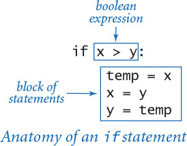
This code puts x and y in ascending order, by exchanging references if necessary.
Most other modern programming languages use some different mechanism to denote statement blocks (such as enclosing statements in matching curly braces). In Python the amount of indentation on each line is consequential, so you need to pay attention to it. For example, contrast these two code fragments, which have slightly different indentation.
if x >= 0: if x >= 0:
stdout.write('not ') stdout.write('not ')
stdout.writeln('negative') stdout.writeln('negative')
The code on the left is an if statement with a one-statement block followed by another statement; the code on the right is an if statement with a two-statement block. If x is greater than or equal to 0, then both fragments write not negative. In contrast, if x is less than 0, then the code on the left writes negative but the code on the right writes nothing at all.
Else clauses
You can add an else clause to an if statement, to express the concept of executing either one statement (or block of statements) or another, depending on whether the boolean expression is True or False, as in this template:
if <boolean expression>:
<block of statements>
else:
<block of statements>
As a simple example of the need for an else clause, the following code assigns the maximum of two int values to the variable maximum. (Alternatively, you can achieve the same result by calling the built-in function max().)
if x > y:
maximum = x
else:
maximum = y
When an if or else block contains only a single statement, for brevity, you can put that statement on the same line as the keyword if or else, as in the third and fourth rows in the table below.
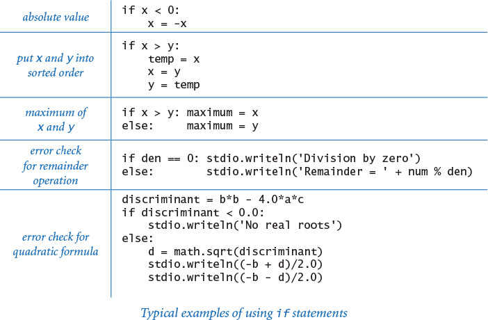
Program 1.3.1 Flipping a fair coin (flip.py)
import random
import stdio
if random.randrange(0, 2) == 0:
stdio.writeln('Heads')
else:
stdio.writeln('Tails')
This program simulates a fair coin flip by writing Heads or Tails, depending on the outcome of random.randrange(). A sequence of flips will have many of the same properties as a sequence that you would get by flipping a fair coin, but it is not a truly random sequence.
% python flip.py
Heads
% python flip.py
Tails
% python flip.py
Tails
The table on the facing page summarizes these and gives two other examples of the use of if and if-else statements. These examples are typical of simple calculations you might need in programs that you compose. Conditional statements are an essential part of programming. As the semantics (meaning) of statements like these is similar to their meanings as natural-language phrases, you will quickly grow used to them.
PROGRAM 1.3.1 (flip.py) is another example of the use of the if-else statement, in this case for the task of simulating a fair coin flip. The body of the program is a single statement, like the other considered so far, but it is worthy of special attention because it introduces an interesting philosophical issue that is valuable to contemplate: can a computer program produce random values? Certainly not, but a program can produce values that have many of the properties of random values.
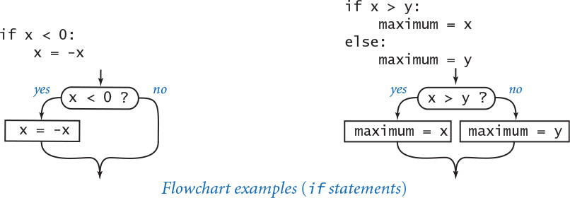
One way to understand control flow is to visualize it with a diagram called a flowchart. Paths through the flowchart correspond to flow-of-control paths in the program. In the early days of computing, when programmers used low-level languages and difficult-to-understand flows of control, flowcharts were an essential part of programming. With modern languages, we use flowcharts just to understand basic building blocks like the if statement.
While statements
Many computations are inherently repetitive. The basic Python construct for handling such computations has the following format:
while <boolean expression>:
<statement 1>
<statement 2>
...
The while statement has the same form as the if statement (the only difference being the use of the keyword while instead of if), but the meaning is quite different. It is an instruction to the computer to behave as follows: if the boolean expression evaluates to False, do nothing; if the expression evaluates to True, execute the block of statements in sequence (just as with if) but then check the expression again, execute the sequence of statements again if the expression evaluates to True, and continue as long as the expression evaluates to True. Thus the flow of control “loops back” to the boolean expression repeatedly. This loop back is evident at the left of the flowchart. (The while statement in this diagram is taken from PROGRAM 1.3.2, which we will examine shortly.) We say that the while statement implements a loop. We refer to the indented statement block within a while statement as the body of the loop and to the boolean expression as the loop-continuation condition. The loop-continuation condition is typically a test about the value of some variable(s), so each while loop is typically preceded by initialization code that sets initial value(s).
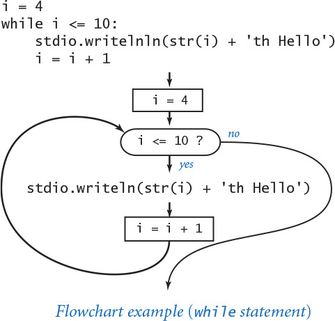
The while statement is equivalent to a sequence of identical if statements:
if <boolean expression>:
<statement 1>
<statement 2>
...
if <boolean expression>:
<statement 1>
<statement 2>
...
if <boolean expression>:
<statement 1>
<statement 2>
...
...
The body of the loop should change one or more variables to make the loop-continuation condition eventually evaluate to False, so that the sequence is broken and the loop terminates.
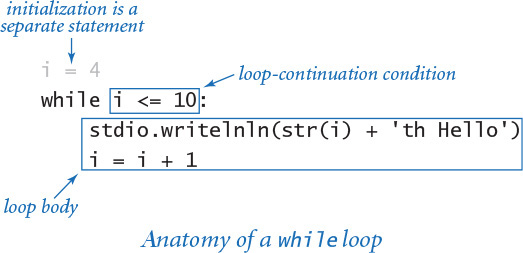
A common programming paradigm involves maintaining an integer value that keeps track of the number of times a loop iterates. We start at some initial value, and then increment the value by 1 each time through the loop, testing whether it exceeds a predetermined maximum before deciding to continue. PROGRAM 1.3.2 (tenhellos.py) is a simple example of this paradigm that uses a while statement. The key to the computation is the statement
i = i + 1
Program 1.3.2 Your first loop (tenhellos.py)
import stdio
stdio.writeln('1st Hello')
stdio.writeln('2nd Hello')
stdio.writeln('3rd Hello')
i = 4
while i <= 10:
stdio.writeln(str(i) + 'th Hello')
i = i + 1
i | loop control counter
This program writes 10 “hellos.” It accomplishes that by using a while loop. After the third line to be written, the lines differ only in the index counting the line written, so we define a variable i to contain that index. After initializing i to 4, we enter into a while loop where we use the i in the stdio.writeln() function call and increment it each time through the loop. After the program writes 10th Hello, i becomes 11 and the loop terminates.
% python tenhellos.py
1st Hello
2nd Hello
3rd Hello
4th Hello
5th Hello
6th Hello
7th Hello
8th Hello
9th Hello
10th Hello

As a mathematical equation, this statement is nonsense, but as a Python assignment statement it makes perfect sense: it says to compute the value i + 1 and then assign the result to the variable i. If i is 4 before the statement executed, then it is 5 afterward; if i is 5 before the statement executes, then it is 6 afterward; and so forth. With the initial condition in tenhellos.py that i starts at 4, the statement block is executed seven times until the sequence is broken, when i finally is greater than 10.
Using the while statement is barely worthwhile for this simple task, but you will soon be addressing tasks where you will need to specify that statements be repeated far too many times to contemplate doing it without loops. There is a profound difference between programs with while statements and programs without them, because while statements allow us to specify a potentially unlimited number of statements to be executed in a program. In particular, the while statement allows us to specify lengthy computations in short programs. This ability opens the door to composing programs for tasks that we could not contemplate addressing without a computer. But there is also a price to pay: as your programs become more sophisticated, they become more difficult to understand.
PROGRAM 1.3.3 (powersoftwo.py) uses a while statement to write a table of the powers of 2. Beyond the loop control counter i, it maintains a variable power that holds the powers of 2 as it computes them. The loop body contains three statements: one to write the current power of 2, one to compute the next power of 2 (multiply the current one by 2), and one to increment the loop control counter.
Incidentally, there are many situations in computer science where it is useful to be familiar with powers of 2. You should know at least the first 10 values in this table and you should note that 210 is about 1,000, 220 is about 1 million, and 230 is about 1 billion.
PROGRAM 1.3.3 is a prototype for many useful computations. By varying the computations that change the accumulated value and the way that the loop control variable is incremented, we can write tables of a variety of functions (see EXERCISE 1.3.10).
It is worthwhile to carefully examine the behavior of programs that use loops by studying a trace of the program. For example, a trace of the operation of powersoftwo.py should show the value of each variable before each iteration of the loop and the value of the conditional expression that controls the loop. Tracing the operation of a loop can be very tedious, but it is nearly always worthwhile to run a trace because it clearly exposes what a program is doing.
Program 1.3.3 Computing powers of 2 (powersoftwo.py)
import sys
import stdio
n = int(sys.argv[1])
power = 1
i = 0
while i <= n:
# Write the ith power of 2.
stdio.writeln(str(i) + ' ' + str(power))
power = 2 * power
i = i + 1
n | loop termination value
i | loop control counter
power | current power of 2
This program accepts an integer n as command-line argument and writes a table containing the first n powers of 2. Each time through the loop, we increment i and double power. We show only the first three and the last three lines of the table; the program write n + 1 lines.
% python powersoftwo.py 5
0 1
1 2
2 4
3 8
4 16
5 32
% python powersoftwo.py 29
0 1
1 2
2 4
...
27 134217728
28 268435456
29 536870912
PROGRAM 1.3.3 is nearly a self-tracing program, because it writes the values of its variables each time through the loop. You can make any program produce a trace of itself by adding appropriate stdio.writeln() statements. Modern programming environments provide sophisticated tools for tracing, but this tried-and-true method is simple and effective. You certainly should add stdio.writeln() statements to the first few loops that you compose, to be sure that they are doing precisely what you expect.
As a more complicated example, suppose that we want to compute the largest power of 2 that is less than or equal to a given positive integer n. If n is 13 we want the result 8; if n is 1000, we want the result 512; if n is 64, we want the result 64; and so forth. This computation is simple to perform with a while loop:
power = 1
while 2*power <= n:
power = 2*power
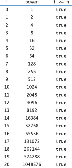
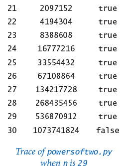
It takes some thought to convince yourself that this simple piece of code produces the desired result. You can do so by making these observations:
• power is always a power of 2.
• power is never greater than n.
• power increases each time through the loop, so the loop must terminate.
• After the loop terminates, 2*power is greater than n.
Reasoning of this sort is often important in understanding how while loops work. Even though many of the loops you will compose are much simpler than this one, you should verify for yourself that each loop you compose will behave as you expect.
The logic behind such arguments is the same whether the loop iterates just a few times, as in tenhellos.py; dozens of times, as in powersoftwo.py; or millions of times, as in several examples that we will soon consider. That leap from a few tiny cases to a huge computation is profound. When composing loops, understanding how the values of the variables change each time through the loop (and checking that understanding by adding statements to trace their values and running the program for a small number of iterations) is essential. Having done so, you can confidently remove those training wheels and truly unleash the power of the computer.
Shorthand assignment notation
Modifying a variable is something that we do so often in programming that modern programming languages like Python provide shorthand notations for the purpose. The most common practice is to abbreviate an assignment statement of the form i = i + 1 with the shorthand notation i += 1. The same notation works for other binary operators, including -, *, and /. For example, most programmers would use power *= 2 instead of power = 2 * power in PROGRAM 1.3.3. Such shortcuts came into widespread use with the C programming language in the 1970s and have become standard. They have survived the test of time because they lead to compact, elegant, and easy-to-understand programs. From this point forward, we will use such augmented assignment statements in our programs whenever possible.
For statements
As you will see, the while statement allows us to compose programs for all manner of applications. Before considering more examples, we will look at an alternative Python construct—the for statement—that allows us even more flexibility when composing programs with loops. This alternative notation is not fundamentally different from the basic while statement, but it often allows us to compose more compact and more readable programs than if we used only while statements.
As noted previously, we often need to design a loop that uses an integer to keep track of the number of times the loop iterates. We initially assign some integer to the variable, and then each time through the loop assign to the variable the integer that is one larger than the previous integer, testing whether the integer exceeds a predetermined maximum before deciding to continue. We call such a loop a counting loop.
In Python, we might implement a counting loop with a while statement using this code pattern:
<variable> = <start>
while <variable> < <stop>:
<block of statements>
<variable> += 1
The for statement is a more succinct way to implement a counting loop. In Python, the for statement has several formats. For now, we consider the following template:
for <variable> in range(<start>, <stop>):
<block of statements>
The <start> and <stop> arguments to the built-in range() function must be integers. When given a statement of this form, Python executes the indented block of statements repeatedly. The first time through the loop <variable> is <start>, the second time <variable> is <start> + 1, and so forth. The final time <variable> is <stop> - 1. In short, a for statement executes its indented statement repeatedly, with <variable> ranging from the integer <start> to the integer <stop> - 1, inclusive. For example, these lines of tenhellos.py (PROGRAM 1.3.2):
i = 4
while i <= 10:
stdio.writeln(str(i) + 'th Hello')
i = i + 1
can be expressed more succinctly using this for statement:
for i in range(4, 11):
stdio.writeln(str(i) + 'th Hello')
If range() has only one argument—that is, the <stop> value—then the <start> value defaults to 0. For example, the following for loop
power = 1
for i in range(n+1):
stdio.writeln(str(i) + ' ' + str(power))
power *= 2
is an improvement over the while loop in powersoftwo.py (PROGRAM 1.3.3).
Choosing among different formulations of the same computation is a matter of each programmer’s taste, as when a writer picks from among synonyms or chooses between using active and passive voice when composing a sentence. You will not find good hard-and-fast rules on how to compose a program any more than you will find such rules on how to compose a paragraph. Your goal should be to find a style that suits you, gets the computation done, and can be appreciated by others. Generally, in this book we use for statements for counting loops, and while statements for other kinds of loops.

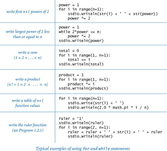
The preceding table includes several code fragments with typical examples of loops used in Python code. Some of these relate to code that you have already seen; others are new code for straightforward computations. To cement your understanding of loops in Python, put each of these code snippets into a program that takes an integer n from the command line (like powersoftwo.py) and run it. Then, compose some loops of your own to perform for similar computations of your own invention, or do some of the early exercises at the end of this section. There is no substitute for the experience gained by running code that you compose yourself, and it is imperative that you develop an understanding of how to compose code that uses loops.
Nesting
The if, while, and for statements have the same status as assignment statements or any other statements in Python. That is, we can use them whenever a statement is called for. In particular, we can nest one or more of them in the body of another. As a first example, divisorpattern.py (PROGRAM 1.3.4) has a for loop whose statements are a for loop (whose statement is an if statement) and a stdio.writeln() statement. It writes a pattern of asterisks where the ith row has an asterisk in each position corresponding to divisors of i (the same holds true for the columns).
PROGRAM 1.3.4 has a complicated control flow, as you can see from its flowchart (shown below). To derive a flowchart like this, it is best to work with a statement-by-statement version of the computation that uses while loops (see EXERCISE 1.3.15), because the for loop version masks the details. This diagram illustrates the importance of using a limited number of simple control structures in programming. With nesting, you can compose loops and conditionals to build programs that are easy to understand even though they may have a complicated control flow. A great many useful computations can be accomplished with just one or two levels of nesting. For example, many programs in this book have the same general structure as divisorpattern.py.

Program 1.3.4 Your first nested loops (divisorpattern.py)
import sys
import stdio
n = int(sys.argv[1])
for i in range(1, n+1):
# Write the ith line.
for j in range(1, n+1):
# Write the jth entry in the ith line.
if (i % j == 0) or (j % i == 0):
stdio.write('* ')
else:
stdio.write(' ')
stdio.writeln(i)
n | number of rows and columns
i | row index
j | column index
This program accepts an integer command-line argument n and writes an n-by-n table with an asterisk in row i and column j if either i divides j or j divides i. The program uses nested for loops. The loop control variables i and j control the computation.
% python divisorpattern.py 3
* * * 1
* * 2
* * 3
% python divisorpattern.py 16
* * * * * * * * * * * * * * * * 1
* * * * * * * * * 2
* * * * * * 3
* * * * * * 4
* * * * 5
* * * * * 6
* * * 7
* * * * * 8
* * * 9
* * * * 10
* * 11
* * * * * * 12
* * 13
* * * * 14
* * * * 15
* * * * * 16

To indicate the nesting, we use indentation in the program code. Again, the indentation is significant in Python (many other programming languages require curly braces or some other notation to indicate nesting). In PROGRAM 1.3.4, we refer to the i loop as the outer loop and the j loop as the inner loop. The inner loop iterates all the way through for each iteration of the outer loop. As usual, the best way to understand a new programming construct like this is to study a trace.
As a second example of nesting, consider a tax preparation program that computes income tax rates. People with no income (or less) pay no income tax; people with income of $0 or more but less than $8,925 pay 10 percent; people with income of $8,925 or more but less than $36,250 pay 15 percent; and so forth. We might accomplish this by using if statements with else clauses, one nested within another:
if income < 0.0:
rate = 0.00
else:
if income < 8925:
rate = 0.10
else:
if income < 36250:
rate = 0.15
else:
if income < 87850:
rate = 0.25
...
In this application, the level of nesting becomes so deep that it makes the code hard to understand. Choosing among several mutually exclusive alternatives in this way is such a common task that an alternative that avoids this deep nesting is appropriate. The Python construct for this purpose is a generalized if statement that allows any number of “else if” clauses of the form
elif <boolean expression>:
<block of statements>
before the “else” clause. When an elif block contains only a single statement, you can put the statement on the same line as the elif keyword for brevity and clarity. With this construct, the code to compute a marginal tax rate is straightforward:
if income < 0: rate = 0.00
elif income < 8925: rate = 0.10
elif income < 36250: rate = 0.15
elif income < 87850: rate = 0.23
elif income < 183250: rate = 0.28
elif income < 398350: rate = 0.33
elif income < 400000: rate = 0.35
else: rate = 0.396
Python evaluates the boolean expressions sequence until reaching one that is True, when its corresponding block of statements is executed. Note that the final else is for the case where none of the conditions is satisfied (the tax rate for the rich, in this case). This construct is a special one that we use often.
Applications
The ability to program with conditionals and loops immediately opens up the full world of computation. To emphasize this fact, we next consider a variety of examples. These examples all involve working with the types of data that we considered in SECTION 1.2, but rest assured that the same mechanisms serve us well for any computational application. The programs are carefully crafted, and by studying and appreciating them, you will be prepared to compose your own programs containing loops.
The examples that we consider here involve computing with numbers. Several of our examples are tied to problems pondered by mathematicians and scientists over the past several centuries. While computers have existed for only 50 years or so, many of the computational methods that we use are based on a rich mathematical tradition tracing back to antiquity.
Finite sum
The computational paradigm used by powersoftwo.py is one that you will use frequently. It uses two variables—one as an index that controls a loop and the other to accumulate a computational result. PROGRAM 1.3.5 (harmonic.py) uses the same paradigm to evaluate the finite sum Hn = 1 + 1/2 + 1/3 + ... + 1/n. These numbers, which are known as the harmonic numbers, arise frequently in discrete mathematics. Harmonic numbers are the discrete analog of the logarithm. They also approximate the area under the curve y = 1/x. You can use PROGRAM 1.3.5 as a model for computing the values of other sums (see EXERCISE 1.3.16).

Program 1.3.5 Harmonic numbers (harmonic.py)
import sys
import stdio
n = int(sys.argv[1])
total = 0.0
for i in range(1, n+1):
# Add the ith term to the sum.
total += 1.0 / i
stdio.writeln(total)
n | number of terms in sum
i | loop control variable
total | cumulated sum
This program accepts integer n as a command-line argument and writes the nth harmonic number. The value is known from mathematical analysis to be about ln(n) + 0.57721 for large n. Note that ln(10,000) ≈ 9.21034.
% python harmonic.py 2
1.5
% python harmonic.py 10
2.9289682539682538
% python harmonic.py 10000
9.787606036044348
Computing the square root
How are functions in Python’s math module, such as math.sqrt(), implemented? PROGRAM 1.3.6 (sqrt.py) illustrates one technique. To compute the square root function, it uses an iterative computation that was known to the Babylonians over 4,000 years ago. It is also a special case of a general computational technique that was developed in the 17th century by Isaac Newton and Joseph Raphson and is widely known as Newton’s method. Under generous conditions on a given function f (x), Newton’s method is an effective way to find roots (values of x for which the function is 0). Start with an initial estimate, t0. Given the estimate ti, compute a new estimate by drawing a line tangent to the curve y = f (x) at the point (ti, f (ti)) and set ti+1 to the x-coordinate of the point where that line hits the x-axis. Iterating this process, we get closer to the root.
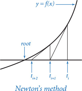
Computing the square root of a positive number c is equivalent to finding the positive root of the function f(x) = x2 – c. For this special case, Newton’s method amounts to the process implemented in sqrt.py (see PROGRAM 1.3.6 and EXERCISE 1.3.17). Start with the estimate t = c. If t is equal to c / t, then t is equal to the square root of c, so the computation is complete. If not, refine the estimate by replacing t with the average of t and c / t. With Newton’s method, we get the value of the square root of 2 accurate to 15 places in just 5 iterations of the loop.
Newton’s method is important in scientific computing because the same iterative approach is effective for finding the roots of a broad class of functions, including many for which analytic solutions are not known (so the Python math module would be no help). Nowadays, we take for granted that we can find whatever values we need of mathematical functions; before computers, scientists and engineers had to use tables or compute values by hand. Computational techniques that were developed to enable calculations by hand needed to be very efficient, so it is not surprising that many of those same techniques are effective when we use computers. Newton’s method is a classic example of this phenomenon.
Another useful approach for evaluating mathematical functions is to use Taylor series expansions (see EXERCISES 1.3.37 and 1.3.38). Evaluating trigonometric functions is a typical application.
Program 1.3.6 Newton’s method (sqrt.py)
import sys
import stdio
EPSILON = 1e-15
c = float(sys.argv[1])
t = c
while abs(t - c/t) > (EPSILON * t):
# Replace t by the average of t and c/t.
t = (c/t + t) / 2.0
stdio.writeln(t)
c | argument
EPSILON | error tolerance
t | estimate of c
This program accepts a positive float c as a command-line argument, and writes the square root of c to 15 decimal places of accuracy. It uses Newton’s method (see text) to compute the square root.
% python sqrt.py 2.0
1.414213562373095
% python sqrt.py 2544545
1595.1630010754388
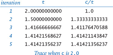

Number conversion
PROGRAM 1.3.7 (binary.py) writes the binary (base 2) representation of the decimal number typed as the command-line argument. It is based on decomposing a number into a sum of powers of 2. For example, the binary representation of 19 is 10011, which is the same as saying that 19 = 16 + 2 + 1. To compute the binary representation of n, we consider the powers of 2 less than or equal to n in decreasing order to determine which belong in the binary decomposition (and therefore correspond to a 1 bit in the binary representation). This process corresponds precisely to using a balance scale to weigh an object, using weights whose values are powers of 2. First, we find the largest weight not heavier than the object. Then, considering the weights in decreasing order, we add each weight to test whether the object is lighter. If so, we remove the weight; if not, we leave the weight and try the next one. Each weight corresponds to a bit in the binary representation of the weight of the object: leaving a weight corresponds to a 1 bit in the binary representation of the object’s weight, and removing a weight corresponds to a 0 bit in the binary representation of the object’s weight.

In binary.py, the variable v corresponds to the current weight being tested, and the variable n accounts for the excess (unknown) part of the object’s weight (to simulate leaving a weight on the balance, we just subtract that weight from n). The value of v decreases through the powers of 2. When v is larger than n, binary.py writes 0; otherwise, it writes 1 and subtracts v from n. As usual, a trace (of the values of n, v, n < v, and the output bit for each loop iteration) can be very useful in helping you to understand the program. Read from top to bottom in the rightmost column of the trace, the output is 10011—the binary representation of 19.
Program 1.3.7 Converting to binary (binary.py)
import sys
import stdio
n = int(sys.argv[1])
# Compute v as the largest power of 2 <= n.
v = 1
while v <= n // 2:
v *= 2
# Cast out powers of 2 in decreasing order.
while v > 0:
if n < v:
stdio.write(0)
else:
stdio.write(1)
n -= v
v //= 2
stdio.writeln()
v | current power of 2
n | current excess
This program writes the binary representation of a positive integer given as the command-line argument, by casting out powers of 2 in decreasing order (see text).
% python binary.py 19
10011
% python binary.py 255
11111111
% python binary.py 512
100000000
% python binary.py 100000000
101111101011110000100000000

Converting data from one representation to another is a frequent theme in composing computer programs. Thinking about conversion emphasizes the distinction between an abstraction (an integer like the number of hours in a day) and a representation of that abstraction (24 or 11000). The irony here is that the computer’s representation of an integer is actually based on its binary representation.
Monte Carlo simulation
Our next example is different in character from the ones we have been considering, but it is representative of a common situation where we use computers to simulate what might happen in the real world so that we can make informed decisions. The specific example that we consider now is from a thoroughly studied class of problems known as gambler’s ruin. Suppose that a gambler makes a series of fair $1 bets, starting with some given initial stake. The gambler always goes broke eventually, but when we set other limits on the game, various questions arise. For example, suppose that the gambler decides ahead of time to walk away after reaching a certain goal. What are the chances that the gambler will win? How many bets might be needed to win or lose the game? What is the maximum amount of money that the gambler will have during the course of the game?
PROGRAM 1.3.8 (gambler.py) is a simulation that can help answer these questions. It performs a sequence of trials, using random.randrange() to simulate the sequence of bets, continuing until the gambler is broke or the goal is reached, and keeping track of the number of wins and the number of bets. After running the experiment for the specified number of trials, the program averages and writes the results. You might wish to run this program for various command-line arguments—not necessarily just to plan your next trip to the casino, but to help you think about the following questions: Is the simulation an accurate reflection of what would happen in real life? How many trials are needed to get an accurate answer? What are the computational limits on performing such a simulation? Simulations are widely used in applications in economics, science, and engineering, and questions of this sort are important in any simulation.

Program 1.3.8 Gambler’s ruin simulation (gambler.py)
import random
import sys
import stdio
stake = int(sys.argv[1])
goal = int(sys.argv[2])
trials = int(sys.argv[3])
bets = 0
wins = 0
for t in range(trials):
# Run one experiment.
cash = stake
while (cash > 0) and (cash < goal):
# Simulate one bet.
bets += 1
if random.randrange(0, 2) == 0:
cash += 1
else:
cash -= 1
if cash == goal:
wins += 1
stdio.writeln(str(100 * wins // trials) + '% wins')
stdio.writeln('Avg # bets: ' + str(bets // trials))
stake | initial stake
goal | walkaway goal
trials | number of trials
bets | bet count
wins | win count
cash | cash on hand
% python gambler.py 10 20 1000
50% wins
Avg # bets: 100
% python gambler.py 50 250 100
19% wins
Avg # bets: 11050
% python gambler.py 500 2500 100
21% wins
Avg # bets: 998071
This program accepts integer command-line arguments stake, goal, and trials. It performs trials experiments, each of which starts with stake dollars and terminates on 0 dollars or goal. Then it writes the percentage of wins and the average number of bets per experiment. The inner while loop simulates a gambler with stake dollars who makes a series of $1 bets, continuing until going broke or reaching goal. The running time of this program is proportional to the total number of bets (trials times the average number of bets). For example, the last experiment shown causes nearly 100 million random numbers to be generated.
In the case of gambler.py, we are verifying classical results from probability theory, which say the probability of success is the ratio of the stake to the goal and that the expected number of bets is the product of the stake and the desired gain (the difference between the goal and the stake). For example, if you want to go to Monte Carlo and try to turn $500 into $2,500, you have a reasonable (20 percent) chance of success, but you should expect to make a million $1 bets! If you try to turn $1 into $1,000, you have a 0.1 percent chance and can expect to be done (ruined, most likely) in about 999 bets (on average).
Simulation and analysis go hand-in-hand, each validating the other. In practice, the value of simulation is that it can suggest answers to questions that might be too difficult to resolve with analysis. For example, suppose that our gambler, recognizing that there will never be enough time to make a million bets, decides ahead of time to set an upper limit on the number of bets. How much money can the gambler expect to take home in that case? You can address this question with an easy change to PROGRAM 1.3.8 (see EXERCISE 1.3.24), but addressing it with mathematical analysis is not so easy.
Factoring
A prime is an integer greater than 1 whose only positive divisors are 1 and itself. The prime factorization of an integer is the multiset of primes whose product is the integer. For example, 3757208 = 2*2*2*7*13*13*397. PROGRAM 1.3.9 (factors.py) computes the prime factorization of any given positive integer. In contrast to many of the other programs that we have seen (which we could do in a few minutes with a calculator or even a pencil and paper), this computation would not be feasible without a computer. How would you go about trying to find the factors of a number like 287994837222311? You might find the factor 17 quickly, but even with a calculator it would take you quite a while to find 1739347.
Although factors.py is compact and straightforward, it certainly will take some thought to convince yourself that it produces the desired result for any given integer. As usual, following a trace that shows the values of the variables at the beginning of each iteration of the outer for loop is a good way to understand the computation. For the case where n is initially 3757208, the inner while loop iterates three times when factor is 2, to remove the three factors of 2; then zero times when factor is 3, 4, 5, and 6, since none of those numbers divides 469651; and so forth.
Program 1.3.9 Factoring integers (factors.py)
import sys
import stdio
n = int(sys.argv[1])
factor = 2
while factor*factor <= n:
while (n % factor) == 0:
# Cast out and write factor.
n //= factor
stdio.write(str(factor) + ' ')
factor += 1
# Any factors of n are greater than or equal to factor.
if n > 1:
stdio.write(n)
stdio.writeln()
n | unfactored part
factor | potential factor
This program writes the prime factorization of any positive integer. The code is simple, but it takes some thought to convince oneself that it is correct (see text).
% python factors.py 3757208
2 2 2 7 13 13 397
% python factors.py 287994837222311
17 1739347 9739789

Tracing the program for a few example inputs clearly reveals its basic operation. To convince ourselves that the program will behave as expected for all inputs, we reason about what we expect each of the loops to do. The inner while loop clearly writes and removes from n all factors of factor. The key to understanding the program is to see that the following invariant holds at the beginning of each iteration of the outer while loop: n has no factors between 2 and factor-1. Thus, if factor is not prime, it will not divide n; if factor is prime, the while loop will do its job and the invariant will continue to hold. We can stop looking for factors when factor*factor is greater than n because if an integer n has a factor, it has one less than or equal to the square root of n.
In a more naïve implementation, we might simply have used the condition (factor < n) to terminate the outer loop. Even given the blinding speed of modern computers, such a decision would have a dramatic effect on the size of the numbers that we could factor. EXERCISE 1.3.26 encourages you to experiment with the program to explore the effectiveness of this simple change. On a computer that can do billions of operations per second, we could factor numbers on the order of 109 in a few seconds; with the (factor*factor <= n) test, we can factor numbers on the order of 1018 in a comparable amount of time. Loops give us the ability to solve difficult problems, but they also give us the ability to construct simple programs that run slowly, so we must always be cognizant of performance issues.
In modern applications such as cryptography, there are important situations where we wish to factor truly huge numbers (with, say, hundreds or thousands of digits). Even for experts, such a computation has so far turned out to be prohibitively difficult even with the use of a computer.
Loop and a half
Sometimes the loop we need does not fit neatly into the flow-control structure of either a for or while loop. For example, suppose we want a loop that repeatedly does the following: execute some sequence of statements, exit the loop if some loop-termination condition is satisfied, and execute some other sequence of statements. That is, we want to position the loop-control condition in the middle of the loop, not at the beginning. This is known as a loop and a half because you must go partway through the loop before reaching the loop-termination test. Python provides the break statement for this purpose. When Python executes a break statement, it immediately exits the (innermost) loop.
For example, consider the problem of generating points that are randomly distributed in the unit disk. We can call random.random() to generate x- and y-coordinates to get points that are randomly distributed in the 2-by-2 square centered at the origin. Most of these points fall within the unit disk, so we just reject those that do not. Since we always want to generate at least one point, we compose a while loop whose loop-continuation condition is always satisfied, generate the random point (x, y) in the 2-by-2 square, and use a break statement to terminate the loop if (x, y) is in the unit disk.
while True:
x = 1.0 + 2.0*random.random()
y = 1.0 + 2.0*random.random()
if x*x + y*y <= 1.0:
break

Since the area of the unit disk is π and the area of the square is 4, the expected number of times the loop is iterated is 4/π (about 1.27).
Experts debate the merits of such internal exits from a loop. When misused, break statements can complicate the flow of control for a loop. However, in situations like this one, alternatives can be complicated (see EXERCISE 1.3.30). Some languages provide a “do–while” statement specifically to handle such cases. In Python, we recommend judicious use of a break statement, when necessary.
Infinite loops
Before you compose programs that use loops, you need to think about the following issue: what if the loop-continuation condition in a while loop is always satisfied? With the statements that you have learned so far, one of two bad things could happen, both of which you need to learn to cope with.
First, suppose that such a loop calls stdout.writeln(). For example, if the loop-continuation condition in tenhellos.py were i > 3 instead of i <= 10, it would always be True. What happens? Nowadays, we use write as an abstraction to mean display in a terminal window, and the result of attempting to display an unlimited number of lines in a terminal window depends on the operating system’s conventions. If your system is set up to have write mean print characters on a piece of paper, you might run out of paper or have to unplug the printer. In a terminal window, you need a “stop writing” operation. Before running programs with loops on your own, you should make sure that you know how to “pull the plug” on an infinite loop of stdout.writeln() calls and then test out that strategy by making the change to tenhellos.py indicated previously and trying to stop it. On most systems, <Ctrl-c> means stop the current program and should do the job.
An infinite loop (with output)
import stdio
i = 4
while i > 3:
stdio.write(i)
stdio.writeln('th Hello')
i += 1
% python infiniteloop1.py
1st Hello
2nd Hello
3rd Hello
5th Hello
6th Hello
7th Hello
8th Hello
9th Hello
10th Hello
11th Hello
12th Hello
13th Hello
14th Hello
...
An infinite loop (with no output)
while True:
x = random.random()
y = random.random()
if x*x + y*y >= 2.0:
break
% python infiniteloop2.py
...
Second, nothing might happen. At least, nothing visible might happen. If your program has an infinite loop that does not produce any output, it will spin through the loop and you will see no results at all. The program will appear to stall. When you find yourself in such a situation, you can inspect the loops to make sure that the loop-termination condition always happens, but the problem may not be easy to identify. One way to locate such a bug is to insert calls to stdout.writeln() to produce a trace. If these calls fall within an infinite loop, this strategy reduces the problem to the case discussed in the previous paragraph, but the output might give you a clue about what to do.
You might not know (or it might not matter) whether a loop is infinite or just very long. If you run gambler.py with arguments such as python gambler.py 100000 200000 100, you may not want to wait for the answer. Later, you will learn to be aware of and to estimate the running time of your programs. SECTION 4.1 introduces this topic.
Why not have Python detect infinite loops and warn us about them? You might be surprised to know that it is not possible to do so, in general. This counterintuitive fact is one of the fundamental results of theoretical computer science.
Summary
For reference, the accompanying table lists the programs that we have considered in this section. They are representative of the kinds of tasks we can address with short programs consisting of if, while, and for statements that process built-in types of data. These types of computations are an appropriate way to become familiar with the basic Python flow-of-control constructs. The time that you spend now working with as many such programs as you can will certainly pay off in the future.
To learn how to use conditionals and loops, you must practice composing and debugging programs with if, while, and for statements. The exercises at the end of this section provide many opportunities for you to begin this process. For each exercise, you will compose a Python program, then run and test it. All programmers know that it is unusual to have a program work as planned the first time it is run, so you will want to have an understanding of your program and an expectation of what it should do, step by step. At first, use explicit traces to check your understanding and expectation. As you gain experience, you will find yourself thinking in terms of what a trace might produce as you compose your loops. Ask yourself the following kinds of questions: What will be the values of the variables after the loop iterates the first time? The second time? The final time? Is there any way this program could get stuck in an infinite loop?
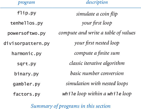
Loops and conditionals are a giant step in our ability to compute: if, while, and for statements take us from simple straight-line programs to an arbitrarily complicated flow of control. In the next several chapters, we will take more giant steps that will allow us to process large amounts of input data and to define and process types of data other than simple numeric types. The if, while, and for statements of this section will play an essential role in the programs that we consider as we take these steps.
A. We repeat this question here to remind you that you should not use = when you really mean == in a conditional expression. The statement x = y assigns y to x, whereas the expression x == y tests whether the two variables currently are equal. In some programming languages, this difference can wreak havoc in a program and be difficult to detect. In Python, assignment statements are not expressions. For example, if we were to make the mistake of typing cash = goal instead of cash == goal in PROGRAM 1.3.8, the compiler would find the bug for us:
% python gambler.py 10 20 1000
File "gambler.py", line 21
if cash = goal:
∧
SyntaxError: invalid syntax
Q. What happens if I leave out the colon in an if, while, or for statement?
A. Python raises a SyntaxError at compile time.
Q. What are the rules for indenting statement blocks?
A. Each statement in a block must have the same indentation; if it does not, Python will raise an IndentationError at compile time. Python programmers commonly use a four-space indentation scheme, which we follow throughout this book.
Q. Should I use tab characters to indent my code?
A. No, you should avoid placing tab characters in your .py files. Many editors, however, offer the option of automatically placing a sequence of spaces into your program when you type the <Tab> key; it’s appropriate to use that option when composing Python programs.
Q. Can I spread a long statement over multiple lines?
A. Yes, but some care is needed because of the way Python treats indentation. If the expression that spans multiple lines is enclosed inside parentheses (or square brackets or curly braces), then there is no need to do anything special. For example, this is a single statement that is spread over three lines:
stdio.write(a0 + a1 + a2 + a3 +
a4 + a5 + a6 + a7 +
a8 + a9)
However, if there is no implied line continuation, you must use the backslash character at the end of each line to be continued.
total = a0 + a1 + a2 + a3 +
a4 + a5 + a6 + a7 +
a8 + a9
Q. Suppose I want to skip over some of code in a loop in some cases, or suppose that I want the body of a conditional statement to be empty, so that no statement is executed. Does Python have language support for such things?
A. Yes, Python provides the continue and pass statements, respectively, for these conditions. However, situations in which they are really necessary are rare, and we do not use them in this book. Also, there is no switch statement in Python (for mutually exclusive alternatives), though one is commonly found in other languages, and no goto statement (for unstructured control flow).
Q. Can I use a non-boolean expression in an if or while statement?
A. Yes, but this is probably not a good idea. Expressions that evaluate to zero or the empty string are considered False; all other numeric and string expressions are considered True.
Q. Are there cases where I must use a for statement but not a while statement, or vice versa?
A. You can use a while statement to implement any kind of loop, but, as defined here, you can use a for statement only for the kind of loop that iterates over a finite sequence of integers. Later (SECTIONS 1.4, 3.3, and 4.4), we will consider other ways to use the for statement.
Q. Can I use the built-in range() function to create a sequence of integers with a step size of some value other than 1?
A. Yes, range() supports an optional third argument step, which defaults to 1. That is, range(start, stop, step) produces the sequence of integers start, start + step, start + 2 * step, and so forth. If step is a positive integer, the sequence continues as long as start + i * step is less than stop; if step is a negative integer, the sequence continues as long as start + i * step is greater than stop. For example, range(0, -100, -1) returns the integer sequence 0, -1, -2, ..., -99.
Q. Can I use floats as arguments to range()?
A. No, all arguments must be integers.
Q. Can I change the loop-index variable within a for loop?
A. Yes, but it will not affect the sequence of integers produced by range(). For example, the following loop writes the 100 integers from 0 to 99:
for i in range(100):
stdio.writeln(i)
i += 10
Q. In a for loop, what is the value of the loop-control variable after the loop terminates?
A. It is the last value of the loop-control variable during the loop. Upon termination of the for loop above, i refers to the integer 109. Using the loop-control variable after the termination of a for loop is generally considered poor style, so we do not do so in any of our programs.
Exercises
1.3.1 Compose a program that takes three integer command-line arguments and writes ‘equal' if all three are equal, and ‘not equal' otherwise.
1.3.2 Compose a more general and more robust version of quadratic.py (PROGRAM 1.2.4) that writes the roots of the polynomial ax2 + bx + c, writes an appropriate message if the discriminant is negative, and behaves appropriately (avoiding division by zero) if a is zero.
1.3.3 Compose a code fragment that takes two float command-line arguments and writes True if both are strictly between 0.0 and 1.0, and False otherwise.
1.3.4 Improve your solution to EXERCISE 1.2.22 by adding code to check that the values of the command-line arguments fall within the ranges of validity of the wind chill formula, as well as code to write an error message if that is not the case.
1.3.5 What is j after each of the following code fragments is executed?
a. j = 0
for i in range(j, 10):
j += i
b. j = 0
for i in range(10):
j += j
c. for j in range(10):
j += j
1.3.6 Redesign tenhellos.py to compose a program hellos.py that takes the number of lines to write as a command-line argument. You may assume that the argument is less than 1000. Hint: Use i % 10 and i % 100 to determine when to use st, nd, rd, or th for writing the ith Hello.
1.3.7 Compose a program fiveperline.py that, using one for loop and one if statement, writes the integers from 1,000 (inclusive) to 2,000 (exclusive) with five integers per line. Hint: Use the % operator.
1.3.8 Generalizing the “uniform random numbers” exercise from SECTION 1.2 (EXERCISE 1.2.27), compose a program stats.py that accepts an integer n as a command-line argument, uses random.random() to write n uniform random numbers between 0 and 1, and then writes their average value, their minimum value, and their maximum value.
1.3.9 In this section, we presented this code to implement the ruler function:
ruler = '1'
stdio.writeln(ruler)
for i in range(2, n+1):
ruler = ruler + ' ' + str(i) + ' ' + ruler
stdio.writeln(ruler)
Describe what happens when you run this code when n is too large—for example, when n is 100.
1.3.10 Compose a program functiongrowth.py that writes a table of the values log2 n, n, n loge n, n2, n3, and 2n for n = 2, 4, 8,16, 32, 64, ..., 2048. To line up columns, use tabs ( characters).
1.3.11 What are m and n after the following code is executed?
n = 123456789
m = 0
while n != 0:
m = (10 * m) + (n % 10)
n /= 10
1.3.12 What does this code write?
f = 0
g = 1
for i in range(16):
stdio.writeln(f)
f = f + g
g = f - g
Solution: Even an expert programmer will tell you that the only way to understand a program like this is to trace it. When you do, you will find that it writes the values 0, 1, 1, 2, 3, 5, 8, 13, 21, 34, 55, 89, 134, 233, 377, and 610. These numbers are the first 16 of the famous Fibonacci sequence, which are defined by the following formulas: F0 = 0, F1 = 1, and Fn = Fn-1 + Fn-2 for n > 1. The Fibonacci sequence arises in a surprising variety of contexts; it has been studied for centuries, and many of its properties are well known. For example, the ratio of successive numbers approaches the golden ratio φ (about 1.618) as n approaches infinity.
1.3.13 Compose a program that takes a command-line argument n and writes all the positive powers of 2 less than or equal to n. Make sure that your program works properly for all values of n. (Your program should write nothing if n is negative.)
1.3.14 Expand your solution to the “Continuously compounded interest” exercise from SECTION 1.2 (EXERCISE 1.2.21) to write a table giving the total amount paid and the remaining principal after each monthly payment.
1.3.15 Compose a version of divisorpattern.py (PROGRAM 1.3.4) that uses while loops instead of for loops.
1.3.16 Unlike the harmonic numbers, the sum 1/12 + 1/22 + ... + 1/n2 does converge to a constant as n grows to infinity. (Indeed, the constant is π2/6, so this formula can be used to estimate the value of π.) Which of the following for loops computes this sum? Assume that n is the integer 1000000 and total is a float initialized to 0.0.
a. for i in range(1, n+1):
total += 1 / (i*i)
b. for i in range(1, n+1):
total += 1.0 / i*i
c. for i in range(1, n+1):
total += 1.0 / (i*i)
d. for i in range(1, n+1):
total += 1.0 / (1.0*i*i)
1.3.17 Show that sqrt.py (PROGRAM 1.3.6) implements Newton’s method for finding the square root of c. Hint: Use the fact that the slope of the tangent to a (differentiable) function f(x) at x = t is f’(t) to find the equation of the tangent line and then use that equation to find the point where the tangent line intersects the x-axis to show that you can use Newton’s method to find a root of any function as follows: at each iteration, replace the estimate t by t – f(t) / f’(t).
1.3.18 Using Newton’s method, develop a program that takes integers n and k as command-line arguments and writes the kth root of n (Hint: See EXERCISE 1.3.17.)
1.3.19 Modify binary.py to create a program kary.py that takes i and k as command-line arguments and converts i to base k. Assume that k is an integer between 2 and 16. For bases greater than 10, use the letters A through F to represent the 11th through 16th digits, respectively.
1.3.20 Compose a code fragment that puts the binary representation of a positive integer n into a String s.
Solution: Working from PROGRAM 1.3.7, we get the solution
s = ''
v = 1
while v <= n//2:
v *= 2
while v > 0:
if n < v:
s += '0'
else:
s += '1'
n -= v
v //= 2
A simpler option is to work from right to left:
s = ''
while n > 0:
s = str(n % 2) + s
n /= 2
Both of these methods are worthy of careful study.
1.3.21 Compose a version of gambler.py that uses two nested while loops or two nested for loops instead of a while loop inside a for loop.
1.3.22 Compose a program gamblerplot.py that traces a gambler’s ruin simulation by writing a line after each bet in which one asterisk corresponds to each dollar held by the gambler.
1.3.23 Modify gambler.py to take an extra command-line argument that specifies the (fixed) probability that the gambler wins each bet. Use your program to try to learn how this probability affects the chance of winning and the expected number of bets. Try a value of p close to 0.5 (say, 0.48).
1.3.24 Modify gambler.py to take an extra command-line argument that specifies the number of bets the gambler is willing to make, so that there are three possible ways for the game to end: the gambler wins, loses, or runs out of time. Add to the output to give the expected amount of money the gambler will have when the game ends. Extra credit: Use your program to plan your next trip to Monte Carlo.
1.3.25 Modify factors.py to write just one copy each of the prime divisors.
1.3.26 Run quick experiments to determine the impact of using the termination condition (i < n) instead of (i *i <= n) in factors.py (PROGRAM 1.3.9). For each method, find the largest n such that when you type in an n-digit number, the program is sure to finish within 10 seconds.
1.3.27 Compose a program checkerboard.py that takes one command-line argument n and uses a loop within a loop to write a two-dimensional n-by-n checkerboard pattern with alternating spaces and asterisks, like the following 5-by-5 pattern:
* * * * *
* * * *
* * * * *
* * * *
* * * * *
1.3.28 Compose a program gcd.py that finds the greatest common divisor (gcd) of two integers using Euclid’s algorithm, which is an iterative computation based on the following observation: if x is greater than y, then if y divides x, the gcd of x and y is y; otherwise, the gcd of x and y is the same as the gcd of x % y and y.
1.3.29 Compose a program relativelyprime.py that takes one command-line argument n and writes an n-by-n table such that there is an * in row i and column j if the gcd of i and j is 1 (i and j are relatively prime), and a space in that position otherwise.
1.3.30 Compose a program that generates a point that is randomly distributed in the unit disk, but without using a break statement. Compare your solution to the one given at the end of this section.
1.3.31 Compose a program that writes the coordinates of a random point (a, b, c) on the surface of a sphere. To generate such a point, use Marsaglia’s method: Start by picking a random point (x, y) in the unit disk using the method described at the end of this section. Then, set a to ![]() , b to
, b to ![]() , and c to 1– 2 (x2 + y2).
, and c to 1– 2 (x2 + y2).
Creative Exercises
1.3.32 Ramanujan’s taxi. S. Ramanujan was an Indian mathematician who became famous for his intuition about numbers. When the English mathematician G. H. Hardy came to visit him in the hospital one day, Hardy remarked that the number of his taxi was 1729, a rather dull number. To which Ramanujan replied, “No, Hardy! No, Hardy! It is a very interesting number. It is the smallest number expressible as the sum of two cubes in two different ways.” Verify this claim by composing a program that takes a command-line argument n and writes all integers less than or equal to n that can be expressed as the sum of two cubes in two different ways. In other words, find distinct positive integers a, b, c, and d such that a3 + b3 = c3 + d3. Use four nested for loops.
1.3.33 Checksums. The International Standard Book Number (ISBN) is a 10-digit code that uniquely specifies a book. The rightmost digit is a checksum digit that can be uniquely determined from the other 9 digits, from the condition that d1 + 2d2 +3d3 + ... + 10d10 must be a multiple of 11 (here di denotes the ith digit from the right). The checksum digit di can be any value from 0 to 10: the ISBN convention is to use the character 'X' to denote 10. Example: The checksum digit corresponding to 020131452 is 5, because 5 is the only value of x between 0 and 10 for which
10·0 + 9·2 + 8·0 + 7·1 + 6·3 + 5·1 +4·4 +3·5 + 2·2 + 1·x
is a multiple of 11. Compose a program that takes a 9-digit integer as a command-line argument, computes the checksum, and writes the ISBN number.
1.3.34 Counting primes. Compose a program primecounter.py that takes a command-line argument n and writes the number of primes less than or equal to n. Use it to write the number of primes less than or equal to 10 million. Note: If you are not careful to make your program efficient, it may not finish in a reasonable amount of time. Later (in SECTION 1.4), you will learn about a more efficient way to perform this computation called the Sieve of Eratosthenes (see PROGRAM 1.4.3).
1.3.35 2D random walk. A two-dimensional random walk simulates the behavior of a particle moving in a grid of points. At each step, the random walker moves north, south, east, or west with probability equal to 1/4, independent of previous moves. Compose a program randomwalker.py that takes a command-line argument n and estimates how long it will take a random walker to hit the boundary of a 2n-by-2n square centered at the starting point.
1.3.36 Median-of-5. Compose a program that takes five distinct integers from the command line and writes the median value (the value such that two of the other integers are smaller and two are larger). Extra credit: Solve the problem with a program that compares values fewer than seven times for any given input.
1.3.37 Exponential function. Assume that x is a float. Compose a code fragment that uses the Taylor series expansion to assign ex = 1 + x + x2/2! + x3/3! + . . . to total.
Solution: The purpose of this exercise is to get you to think about how a library function like math.exp() might be implemented in terms of elementary operators. Try solving it, then compare your solution with the one developed here.
We start by considering the problem of computing one term. Suppose that x is a float and n is an integer. The following code assigns xn / n ! to term using the direct method of having one loop for the numerator and another loop for the denominator, then dividing the results:
num = 1.0
den = 1.0
for i in range(1, n+1):
num *= x
for i in range(1, n+1):
den *= i
term = num / den
A better approach is to use just a single for loop:
term = 1.0
for i in range(1, n+1):
term *= x / i
Besides being more compact and elegant, the latter solution is preferable because it avoids inaccuracies caused by computing with huge numbers. For example, the two-loop approach breaks down for values like x = 10 and n = 100 because 100! is too large to represent accurately as a float.
To compute ex, we nest this for loop within another for loop:
term = 1.0
total = 0.0
n = 1
while total != total + term:
total += term
term = 1.0
for i in range(1, n+1):
term *= x / i
n += 1
The number of times the while loop iterates depends on the relative values of the next term and the accumulated sum. Once total stops changing, we leave the loop. (This strategy is more efficient than using the termination condition (term > 0) because it avoids a significant number of iterations that do not change the value of the total.) This code is effective, but it is inefficient because the inner for loop recomputes all the values it computed on the previous iteration of the outer for loop. Instead, we can make use of the term that was added in on the previous loop iteration and solve the problem with a single while loop:
term = 1.0
total = 0.0
n = 1
while total != total + term:
total += term
term *= x/n
n += 1
1.3.38 Trigonometric functions. Compose programs sine.py and cosine.py that compute the sine and cosine functions using their Taylor series expansions sin x = x – x3/3! + x5/5! – ... and cos x = 1 – x2/2! + x4/4! – . . .
1.3.39 Experimental analysis. Run experiments to determine the relative costs of math.exp() and the three approaches from EXERCISE 1.3.37 for computing ex: the direct method with nested for loops, the improvement with a single while loop, and the latter with the termination condition (term > 0). Use trial-and-error with a command-line argument to determine how many times your computer can perform each computation in 10 seconds.
1.3.40 Pepys’s problem. In 1693 Samuel Pepys asked Isaac Newton which is more likely: getting 1 at least once when rolling a fair die six times or getting 1 at least twice when rolling it 12 times. Compose a program that could have provided Newton with a quick answer.
1.3.41 Game simulation. In the 1970s game show Let’s Make a Deal, a contestant is presented with three doors. Behind one of them is a valuable prize. After the contestant chooses a door, the host opens one of the other two doors (never revealing the prize, of course). The contestant is then given the opportunity to switch to the other unopened door. Should the contestant do so? Intuitively, it might seem that the contestant’s initial choice door and the other unopened door are equally likely to contain the prize, so there would be no incentive to switch. Compose a program montehall.py to test this intuition by simulation. Your program should take a command-line argument n, play the game n times using each of the two strategies (switch or do not switch), and write the chance of success for each of the two strategies.
1.3.42 Chaos. Compose a program to study the following simple model for population growth, which might be applied to study fish in a pond, bacteria in a test tube, or any of a host of similar situations. We suppose that the population ranges from 0 (extinct) to 1 (maximum population that can be sustained). If the population at time t is x, then we suppose the population at time t + 1 to be rx(1–x), where the parameter r, known as the fecundity parameter, controls the rate of growth. Start with a small population—say, x = 0.01—and study the result of iterating the model, for various values of r. For which values of r does the population stabilize at x = 1 – 1/r ? Can you say anything about the population when r is 3.5? 3.8? 5?
1.3.43 Euler’s sum-of-powers conjecture. In 1769 Leonhard Euler formulated a generalized version of Fermat’s Last Theorem, conjecturing that at least n nth powers are needed to obtain a sum that is itself an nth power, for n > 2. Compose a program to disprove Euler’s conjecture (which stood until 1967), using a quintuply nested loop to find four positive integers whose 5th power sums to the 5th power of another positive integer. That is, find five integers a, b, c, d, and e such that a5 + b5 + c5 + d5 = e5.