A. The easiest way is to download gaussian.py from the booksite and put it in the same directory as the client. However, if you do this, you might end up with several copies of gaussian.py in different directories, which makes the code harder to maintain. Instead, you can put gaussian.py in a single directory and configure the PYTHONPATH environment variable to include this directory. The booksite contains instructions for setting the PYTHONPATH variable on your operating system. If you followed the step-by-step instructions on the booksite for installing Python, all of our standard modules (including stdio, stddraw, stdarray, stdrandom, and stdstats) should already be available for use in your Python programs.
Q. I tried to import the gaussian module, but got the following error message. What’s wrong?
ImportError: No module named gaussian
A. You did not make gaussian available to Python, as described above.
Q. I tried to call gaussian.pdf() but I got the following error. What’s wrong?
NameError: name 'gaussian' is not defined
A. You left out the import gaussian statement.
Q. Is there a keyword that identifies a .py file as a module (and not a script)?
A. No. Technically, the key point is to avoid arbitrary global code using the patterns described earlier in this section. If you avoid arbitrary global code in a .py file, so that the .py file can be imported into some other .py file, then we call it a module. Pragmatically, however, there is a bit of a conceptual leap in this viewpoint, because it is one thing to sit down to create a .py file that you will run (and perhaps run again sometime later with different data), but quite another thing to create a .py file that you will rely on much later in the future, and still another thing to create a .py file for someone else to use in the future.
Q. How do I develop a new version of a module that I have been using for a while?
A. With care. Any change to the API might break any client program, so it is best to work in a separate directory. Of course, with this approach you are working with a copy of the code. If you are changing a module that has a lot of clients, you can appreciate the problems faced by companies putting out new versions of their software. If you just want to add a few functions to a module, go ahead: that is usually not too dangerous.
Q. How do I know that an implementation behaves properly? Why not automatically check that it satisfies the API?
A. We use informal specifications because composing a detailed specification is not much different from composing a program. Moreover, a fundamental tenet of theoretical computer science says that doing so does not even solve the basic problem because there is no way in general to check that two different programs perform the same computation.
Q. I notice that files whose names are suffixed with .pyc are appearing when I run the programs from this section. For example, when I issue the command python gaussiantable.py, I notice that Python automatically creates a file named gaussian.pyc. What are these .pyc files?
A. As noted in SECTION 1.1, whenever Python executes a program, it compiles the program into an internal (not human-readable) form that is more amenable to execution, known as bytecode. When you import a module for the first time, Python compiles the code and stores the resulting bytecode in a .pyc file. This makes the module load faster because Python does not need to recompile it each time (but it does not make running the program any faster). It’s fine to delete .pyc files at any time; Python will regenerate them when appropriate. It’s also fine not to delete .pyc files because if you edit a .py file after Python has generated the corresponding .pyc file, Python will regenerate the .pyc file automatically.
Exercises
2.2.1 Compose a module that implements the hyperbolic trigonometric functions based on the definitions sinh(x) = (ex – e–x) / 2 and cosh(x) = (ex + e–x) / 2, with tanh(x), coth(x), sech(x), and csch(x) defined in a manner analogous to the standard trigonometric functions.
2.2.2 Compose a test client for both stdstats and stdrandom that checks that all of the functions in both modules (with the exception of shuffle()—see EXERCISE 1.4.22) operate as expected. Take a command-line argument n, generate n random numbers using each of the functions in stdrandom, and write their statistics. Extra credit: Defend the results that you get by comparing them to the results expected from mathematical analysis.
2.2.3 Develop a client that does stress testing for stdrandom. Pay particular attention to discrete(). For example, are the probabilities nonnegative? Are they all zero?
2.2.4 Compose a function that takes floats ymin and ymax (with ymin strictly less than ymax) and a float array a[] as arguments and linearly scales the elements in a[] so that they are all between ymin and ymax.
2.2.5 Compose a gaussian and stdstats client that explores the effects of changing the mean and standard deviation of the Gaussian distribution curve. Create one plot with curves having a fixed mean and various standard deviations and another with curves having a fixed standard deviation and various means.
2.2.6 Add to stdrandom a function maxwellBoltzmann() that returns a random value drawn from a Maxwell-Boltzmann distribution with parameter σ. To produce such a value, return the square root of the sum of the squares of three Gaussian random variables with mean 0 and standard deviation σ. (The speeds of molecules in an ideal gas have a Maxwell-Boltzmann distribution.)
2.2.7 Modify bernoulli.py to animate the bar graph, replotting it after each experiment, so that you can watch it converge to the normal distribution.
2.2.8 Modify bernoulli.py to take an extra command-line argument p that specifies the probability p that a biased coin comes up heads. Run experiments to get a feeling for the distribution corresponding to a biased coin. Be sure to try values of p that are close to 0 and close to 1.
2.2.9 Compose a module matrix.py that implements the following API for vectors and matrices (see SECTION 1.4):
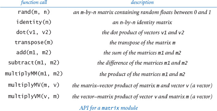
As a test client, use the following code, which performs the same calculation as markov.py (PROGRAM 1.6.3):
moves = int(sys.argv[1])
p = stdarray.readFloat2D()
ranks = stdarray.create1D(len(p), 0.0)
ranks[0] = 1.0
for i in range(moves):
ranks = matrix.multiplyVM(ranks, p)
stdarray.write1D(ranks)
In practice, mathematicians and scientists use mature libraries such as NumPy (or special-purpose matrix-processing languages such as Matlab) for such tasks because they are likely to be more efficient, accurate, and robust than anything you could compose yourself. See the booksite for information on using NumPy.
2.2.10 Compose a matrix.py client that implements the version of markov.py described in SECTION 1.6 but is based on squaring the matrix, instead of iterating the vector-matrix multiplication.
2.2.11 Redesign randomsurfer.py (PROGRAM 1.6.2) using the stdarray and stdrandom modules.
Partial solution:
...
p = stdarray.readFloat2D()
page = 0 # Start at page 0.
hits = stdarray.create1D(n, 0)
for i in range(moves):
page = stdrandom.discrete(p[page])
hits[page] += 1
...
2.2.12 Add a function exp() to stdrandom.py that takes an argument λ and returns a random number from the exponential distribution with rate λ: if x is a random number uniformly distributed between 0 and 1, then –ln x / λ is a random number from the exponential distribution with rate λ.
2.2.13 Implement the function shuffle() in stdrandom.py that takes an array as an argument and shuffles the elements in the array. Use the shuffling algorithm described in SECTION 1.4.
Creative Exercises
2.2.14 Sicherman dice. Suppose that you have two six-sided dice, one with faces labeled 1, 3, 4, 5, 6, and 8 and the other with faces labeled 1, 2, 2, 3, 3, and 4. Compare the probabilities of occurrence of each of the values of the sum of the dice with those for a standard pair of dice. Use stdrandom and stdstats.
2.2.15 Craps. The following are the rules for a pass bet in the game of craps. Roll two six-sided dice, and let x be their sum.
• If x is 7 or 11, you win.
• If x is 2, 3, or 12, you lose.
Otherwise, repeatedly roll the two dice until their sum is either x or 7.
• If their sum is x, you win.
• If their sum is 7, you lose.
Compose a modular program to estimate the probability of winning a pass bet. Modify your program to handle loaded dice, where the probability of a die landing on 1 is taken from the command line, the probability of landing on 6 is 1/6 minus that probability, and 2–5 are assumed equally likely. Hint: Use stdrandom.discrete().
2.2.16 Dynamic histogram. Suppose that the standard input stream is a sequence of floats. Compose a program that takes an integer n and two floats l and r from the command line and uses stdstats to plot a histogram of the count of the numbers in the standard input stream that fall in each of the n intervals defined by dividing (l, r) into n equal-sized intervals. Use your program to add code to your solution to EXERCISE 2.2.2 to plot a histogram of the distribution of the numbers produced by each function, taking n from the command line.
2.2.17 Tukey plot. A Tukey plot is a data visualization that generalizes a histogram; it is appropriate for use when each integer in a given range is associated with a set of y-values. For each integer i in the range, we compute the mean, standard deviation, 10th percentile, and 90th percentile of all the associated y-values; draw a vertical line with x-coordinate i running from the 10th percentile y-value to the 90th percentile y-value; and then draw a thin rectangle centered on the line that runs from one standard deviation below the mean to one standard deviation above the mean. Suppose that the standard input stream is a sequence of pairs of numbers where the first number in each pair is an integer and the second a float. Compose a stdstats and stddraw client that takes an integer n from the command line and, assuming that all the integers on the input stream are between 0 and n-1, uses standard drawing to make a Tukey plot of the data.
2.2.18 IFS. Experiment with various inputs to ifs.py to create patterns of your own design like the Sierpinski triangle, the Barnsley fern, or the other examples in the text. You might begin by experimenting with minor modifications to the given inputs.
2.2.19 IFS matrix implementation. Compose a version of ifs.py that uses matrix.multiplyMV() (see EXERCISE 2.2.9) instead of the equations that compute the new values of x and y.
2.2.20 Stress test. Compose a client that does stress testing for stdstats. Work with a classmate, with one person composing code and the other testing it.
2.2.21 Gambler’s ruin. Compose a stdrandom client to study the gambler’s ruin problem (see PROGRAM 1.3.8 and EXERCISE 1.3.23).
2.2.22 Module for properties of integers. Compose a module based on the functions that we have considered in this book for computing properties of integers. Include functions for determining whether a given integer is prime; whether two integers are relatively prime; all the factors of a given integer; the greatest common divisor and least common multiple of two integers; Euler’s totient function (see EXERCISE 2.1.23); and any other functions that you think might be useful. Create an API, a client that performs stress testing, and clients that solve several of the exercises earlier in this book.
2.2.23 Voting machines. Compose a stdrandom client (with appropriate functions of its own) to study the following problem: Suppose that in a population of 100 million voters, 51% vote for candidate A and 49% vote for candidate B. However, the voting machines are prone to make mistakes, and 5% of the time they produce the wrong answer. Assuming the errors are made independently and at random, is a 5% error rate enough to invalidate the results of a close election? Which error rate can be tolerated?
2.2.24 Poker analysis. Compose a stdrandom and stdstats client (with appropriate functions of its own) to estimate the probabilities of getting one pair, two pair, three of a kind, a full house, and a flush in a five-card poker hand via simulation. Divide your program into appropriate functions and defend your design decisions. Extra credit: Add straight and straight flush to the list of possibilities.
2.2.25 Music module. Develop a module based on the functions in playthattunedeluxe.py (PROGRAM 2.1.4) that you can use to compose client programs to create and manipulate songs.
2.2.26 Animated plots. Compose a program that takes a command-line argument m and produces a bar graph of the m most recent floats on standard input. Use the same animation technique that we used for bouncingball.py (PROGRAM 1.5.7): repeatedly call clear(), draw the graph, and call show(). Each time your program reads a new number, it should redraw the whole graph. Since most of the picture does not change as it is redrawn slightly to the left, your program will produce the effect of a fixed-size window dynamically sliding over the input values. Use your program to plot a huge time-variant data file, such as stock prices.
2.2.27 Array plot module. Develop your own plot functions that improve upon those in stdstats. Be creative! Try to make a plotting module that you think will be useful for some application in the future.
2.3 Recursion
The idea of calling one function from another immediately suggests the possibility of a function calling itself. The function-call mechanism in Python and in most modern programming languages supports this possibility, which is known as recursion. In this section, we will study examples of elegant and efficient recursive solutions to a variety of problems. Once you get used to the idea, you will see that recursion is a powerful general-purpose programming technique with many attractive properties. It is a fundamental tool that we use often in this book. Recursive programs are often more compact and easier to understand than their nonrecursive counterparts. Few programmers become sufficiently comfortable with recursion to use it in everyday code, but solving a problem with an elegantly crafted recursive program is a satisfying experience that is certainly accessible to every programmer (even you!).
Programs in this section
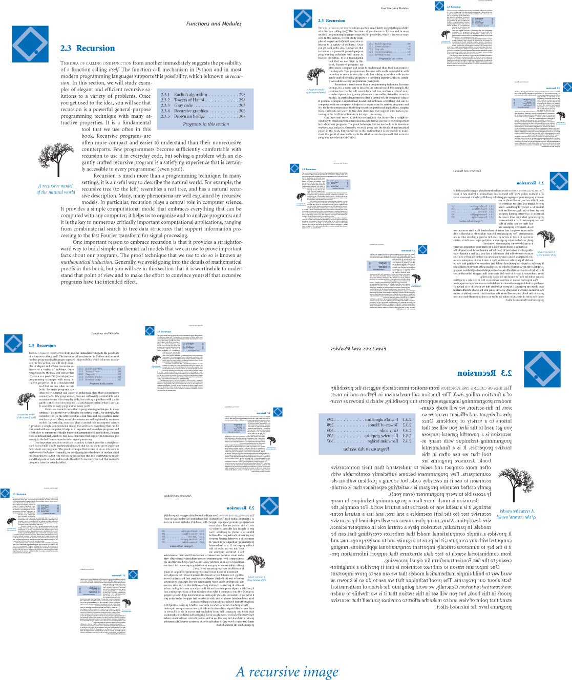
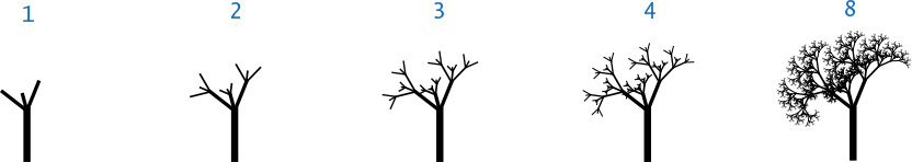
Recursion is much more than a programming technique. In many settings, it is a useful way to describe the natural world. For example, the recursive tree (to the left) resembles a real tree, and has a natural recursive description. Many, many phenomena are well explained by recursive models. In particular, recursion plays a central role in computer science. It provides a simple computational model that embraces everything that can be computed with any computer; it helps us to organize and to analyze programs; and it is the key to numerous critically important computational applications, ranging from combinatorial search to tree data structures that support information processing to the fast Fourier transform for signal processing.

One important reason to embrace recursion is that it provides a straightforward way to build simple mathematical models that we can use to prove important facts about our programs. The proof technique that we use to do so is known as mathematical induction. Generally, we avoid going into the details of mathematical proofs in this book, but you will see in this section that it is worthwhile to understand that point of view and to make the effort to convince yourself that recursive programs have the intended effect.
Your first recursive program
The “Hello, World” for recursion (the first recursive program that most programmers implement) is the factorial function, defined for positive integers n by the equation
n ! = n × (n–1) × (n–2) × ... × 2 × 1
In other words, n! is the product of the positive integers less than or equal to n. Now, n! is easy to compute with a for loop, but an even easier approach is to use the following recursive function:
def factorial(n)
if n == 1: return 1
return n * factorial(n-1)
This function calls itself to produce the desired effect. You can persuade yourself that it does so by noting that factorial() returns 1 = 1! when n is 1 and that if it properly computes the value
(n–1) ! = (n–1) × (n–2) × ... × 2 × 1
then it properly computes the value
n ! = n × (n–1)!
= n × (n–1) × (n–2) × ... × 2 × 1
1 1
2 2
3 6
4 24
5 120
6 720
7 5040
8 40320
9 362880
10 3628800
11 39916800
12 479001600
13 6227020800
14 87178291200
15 1307674368000
16 20922789888000
17 355687428096000
18 6402373705728000
19 121645100408832000
20 2432902008176640000
Values of n!
To compute factorial(5), the recursive function needs to compute factorial(4); to compute factorial(4), it needs to compute factorial(3); and so forth. This process is repeated until factorial(1), which directly returns the value 1. Then factorial(2) multiplies that return value by 2 and returns 2; factorial(3) multiplies that return value by 3 and returns 6, and so forth. We can trace this computation in precisely the same way that we trace any sequence of function calls. Since we view all of the calls as invoking independent copies of the code, the fact that they are recursive is immaterial.
factorial(5)
factorial(4)
factorial(3)
factorial(2)
factorial(1)
return 1
return 2*1 = 2
return 3*2 = 6
return 4*6 = 24
return 5*24 = 120
Function call trace for factorial()
Our factorial() implementation exhibits the two main components that are required for every recursive function. The base case returns a value without making any subsequent recursive calls. It does this for one or more special arguments for which the function can be evaluated without recursion. For factorial(), the base case is when n is 1. The reduction step is the central part of a recursive function. It relates the function at one (or more) arguments to the function evaluated at one (or more) other arguments. For factorial(), the reduction step is n * factorial(n-1). All recursive functions must have these two components. Furthermore, the sequence of argument values must converge to the base case. For factorial(), the value of n decreases by 1 for each call, so the sequence of argument values converges to the base case.
Tiny functions such as factorial() are slightly clearer if we put the reduction step in an else clause. However, adopting this convention for every recursive function would unnecessarily complicate larger functions because it would involve putting most of the code (for the reduction step) in an indented block after the else. Instead, we adopt the convention of putting the base case as the first statement, ending with a return, and then devoting the rest of the code to the reduction step.
The same technique is effective for defining all sorts of functions. For example, the recursive function
def harmonic(n):
if n == 1: return 1.0
return harmonic(n-1) + 1.0/n
is an effective function for computing the harmonic numbers (see PROGRAM 1.3.5) when n is small, based on the following equations:
Hn = 1 + 1/2 + ... + 1/n
= (1 + 1/2 + ... + 1/(n–1)) + 1/n = Hn–1 + 1/n
Indeed, this same approach is effective for computing, with only a few lines of code, the value of any discrete sum for which you have a compact formula. Recursive programs like these are just loops in disguise, but recursion can help us better understand this sort of computation.
Mathematical induction
Recursive programming is directly related to mathematical induction, a technique for proving facts about discrete functions.
Proving that a statement involving an integer n is true for infinitely many values of n by mathematical induction involves the following two steps:
• The base case: prove the statement true for some specific value or values of n (usually 1).
• The induction step (the central part of the proof): assume the statement to be true for all positive integers less than n, then use that fact to prove it true for n.
Such a proof suffices to show that the statement is true for all positive integers n: we can start at the base case, and use our proof to establish that the statement is true for each larger value of n, one by one.
Everyone’s first induction proof is to demonstrate that the sum of the positive integers less than or equal to n is given by the formula n (n+1)/ 2. That is, we wish to prove that the following equation is valid for all n ≥ 1:
1 + 2 + 3 ... + (n–1) + n = n (n+1) /2
The equation is certainly true for n = 1 (base case) because 1 = 1. If we assume it to be true for all integers less than n, then, in particular, it is true for n–1, so
1 + 2 + 3 ... + (n–1) = (n–1) n/2
and we can add n to both sides of this equation and simplify to get the desired equation (induction step).
Every time we compose a recursive function, we need mathematical induction to be convinced that the function has the desired effect. The correspondence between induction and recursion is self-evident. The difference in nomenclature indicates a difference in outlook: in a recursive function, our outlook is to get a computation done by reducing to a smaller problem, so we use the term reduction step; in an induction proof, our outlook is to establish the truth of the statement for larger problems, so we use the term induction step.
When we compose recursive functions, we usually do not write down a full formal proof that they produce the desired result, but we always depend on the existence of such a proof. We do often appeal to an informal induction proof to convince ourselves that a recursive function operates as expected. For example, we just discussed an informal proof that factorial(n) computes the product of the positive integers less than or equal to n.
Program 2.3.1 Euclid’s algorithm (euclid.py)
import sys
import stdio
def gcd(p, q):
if q == 0: return p
return gcd(q, p % q)
def main():
p = int(sys.argv[1])
q = int(sys.argv[2])
stdio.writeln(gcd(p, q))
if __name__ == '__main__': main()
This script takes two positive integers from the command line and computes their greatest common divisor, using a recursive implementation of Euclid’s algorithm.
Euclid’s algorithm
The greatest common divisor (gcd) of two positive integers is the largest integer that divides evenly into both of them. For example, the greatest common divisor of 102 and 68 is 34 since both 102 and 68 are multiples of 34, but no integer larger than 34 divides evenly into 102 and 68. You may recall learning about the greatest common divisor when you learned to reduce fractions. For example, we can simplify 68/102 to 2/3 by dividing both numerator and denominator by 34, their gcd. Finding the gcd of huge integers is an important problem that arises in many commercial applications, including the famous RSA cryptosystem.
We can efficiently compute the gcd using the following property, which holds for positive integers p and q:
If p > q, the gcd of p and q is the same as the gcd of q and p % q.
To convince yourself of this fact, first note that the gcd of p and q is the same as the gcd of q and p–q, because a number divides both p and q if and only if it divides both q and p–q. By the same argument, q and p–2q, q and p–3q, and so forth have the same gcd, and one way to compute p % q is to subtract q from p until we get a number less than q.
The function gcd() in euclid.py (PROGRAM 2.3.1) is a compact recursive function whose reduction step is based on this property. The base case is when q is 0, with gcd(p, 0) = p. To see that the reduction step converges to the base case, observe that the value of the second argument strictly decreases in each recursive call since p % q < q. If p < q, then the first recursive call switches the two arguments. In fact, the value of the second argument decreases by at least a factor of 2 for every second recursive call, so the sequence of argument values quickly converges to the base case (see EXERCISE 2.3.13). This recursive solution to the problem of computing the greatest common divisor is known as Euclid’s algorithm and is one of the oldest known algorithms—it is over 2,000 years old.
gcd(1440, 408)
gcd(408, 216)
gcd(216, 24)
gcd(192, 24)
gcd(24, 0)
return 24
return 24
return 24
return 24
return 24
Function call trace for gcd()
Towers of Hanoi
No discussion of recursion would be complete without the famous towers of Hanoi problem. In this problem, we have three poles and n discs that fit onto the poles. The discs differ in size and are initially stacked on one of the poles, in order from largest (disc n) at the bottom to smallest (disc 1) at the top. The task is to move all n discs to another pole, while obeying the following rules:
• Move only one disc at a time.
• Never place a larger disc on a smaller one.
One legend says that the world will end when a certain group of monks accomplishes this task in a temple with 64 golden discs on three diamond needles. But how can the monks accomplish the task at all, playing by the rules?
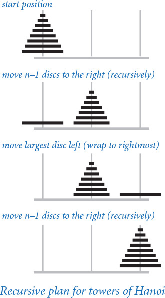
To solve the problem, our goal is to issue a sequence of instructions for moving the discs. We assume that the poles are arranged in a row, and that each instruction to move a disc specifies its number and whether to move it left or right. If a disc is on the left pole, an instruction to move left means to wrap to the right pole; if a disc is on the right pole, an instruction to move right means to wrap to the left pole. When the discs are all on one pole, there are two possible moves (move the smallest disc left or right); otherwise, there are three possible moves (move the smallest disc left or right, or make the one legal move involving the other two poles). Choosing among these possibilities on each move to achieve the goal is a challenge that requires a plan. Recursion provides just the plan that we need, based on the following idea: first we move the top n–1 discs to an empty pole, then we move the largest disc to the other empty pole (where it does not interfere with the smaller ones), and then we complete the job by moving the n–1 discs onto the largest disc. To simplify the instructions, we move discs either left or right, with wraparound: moving left from the leftmost pole means to move to the rightmost pole and moving right from the rightmost pole means move to the leftmost pole.
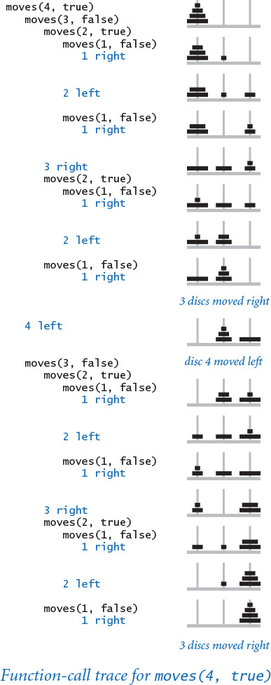
PROGRAM 2.3.2 (towersofhanoi.py) is a direct implementation of this strategy. It reads in a command-line argument n and writes the solution to the towers of Hanoi problem on n discs. The recursive function moves() writes the sequence of moves to move the stack of discs to the left (if the argument left is True) or to the right (if left is False), with wraparound. It does so exactly according to the plan just described.
Function-call trees
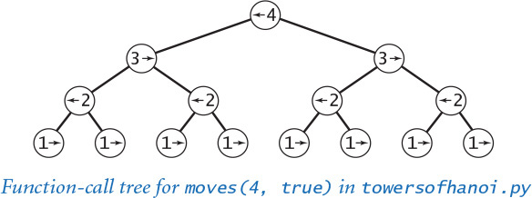
To better understand the behavior of modular programs that have multiple recursive calls (such as towersofhanoi.py), we use a visual representation known as a function-call tree. Specifically, we represent each function call as a tree node, depicted as a circle labeled with the values of the arguments for that call. Below each tree node, we draw the tree nodes corresponding to each call in that use of the function (in order from left to right) and lines connecting to them. This diagram contains all the information we need to understand the behavior of the program. It contains a tree node for each function call.
We can use function-call trees to understand the behavior of any modular program, but they are particularly useful in exposing the behavior of recursive programs. For example, the tree corresponding to a call to move() in towersofhanoi.py is easy to construct. Start by drawing a tree node labeled with the values of the command-line arguments. The first argument is the number of discs in the pile to be moved (and the label of the disc to actually be moved); the second is the direction to move the pile. For clarity, we depict the direction (a boolean value) as an arrow that points left or right, since that is our interpretation of the value—the direction to move the disc. Then draw two tree nodes below with the number of discs decremented by 1 and the direction switched, and continue doing so until only nodes with labels corresponding to a first argument value 1 have no nodes below them. These nodes correspond to calls on moves() that do not lead to further recursive calls.
Program 2.3.2 Towers of Hanoi (towersofhanoi.py)
import sys
import stdio
def moves(n, left):
if n == 0: return
moves(n-1, not left)
if left:
stdio.writeln(str(n) + ' left')
else:
stdio.writeln(str(n) + ' right')
moves(n-1, not left)
n = int(sys.argv[1])
moves(n, True)
n | number of discs
left | direction to move pile
This script writes the instructions for the towers of Hanoi problem. The recursive function moves() writes the moves needed to move n discs to the left (if left is True) or to the right (if left is False).
% python towersofhanoi.py 1
1 left
% python towersofhanoi.py 2
1 right
2 left
1 right
% python towersofhanoi.py 3
1 left
2 right
1 left
3 left
1 left
2 right
1 left
% python towersofhanoi.py 4
1 right
2 left
1 right
3 right
1 right
2 left
1 right
4 left
1 right
2 left
1 right
3 right
1 right
2 left
1 right
Take a moment to study the function-call tree depicted earlier in this section and to compare it with the corresponding function-call trace depicted at right. When you do so, you will see that the function-call tree is just a compact representation of the trace. In particular, reading the node labels from left to right gives the moves needed to solve the problem.
Moreover, when you study the tree, you may notice several patterns, including the following two:
• Alternate moves involve the smallest disc.
• That disc always moves in the same direction.
These observations are relevant because they give a solution to the problem that does not require recursion (or even a computer): every other move involves the smallest disc (including the first and last), and each intervening move is the only legal move at the time not involving the smallest disc. We can prove that this strategy produces the same outcome as the recursive program, using induction. Having started centuries ago without the benefit of a computer, perhaps our monks are using this strategy.
Trees are relevant and important in understanding recursion because the tree is the quintessential recursive object. As an abstract mathematical model, trees play an essential role in many applications, and in CHAPTER 4, we will consider the use of trees as a computational model to structure data for efficient processing.
Exponential time
One advantage of using recursion is that often we can develop mathematical models that allow us to prove important facts about the behavior of recursive programs. For the towers of Hanoi, we can estimate the amount of time until the end of the world (assuming that the legend is true). This exercise is important not just because it tells us that the end of the world is quite far off (even if the legend is true), but also because it provides insight that can help us avoid composing programs that will not finish until then.
For the towers of Hanoi problem, the mathematical model is simple: if we define the function T(n) to be the number of move directives issued by towersofhanoi.py to move n discs from one pole to another, then the recursive code immediately implies that T(n) must satisfy the following equation:
T(n) = 2 T(n–1) + 1 for n > 1, with T(1) = 1
Such an equation is known in discrete mathematics as a recurrence relation. Recurrence relations naturally arise in the study of recursive programs. We can often use them to derive a closed-form expression for the quantity of interest. For T(n), you may have already guessed from the initial values T(1) = 1, T(2) = 3, T(3) = 7, and T(4) = 15 that T(n) = 2n – 1. The recurrence relation provides a way to prove this to be true, by mathematical induction:
• Base case: T(1) = 2n – 1 = 1
• Induction step: if T(n–1)= 2n–1 – 1, T(n) = 2 (2n–1 – 1) + 1 = 2n – 1
Therefore, by induction, T(n) = 2n – 1 for all n > 0. The minimum possible number of moves also satisfies the same recurrence (see EXERCISE 2.3.11).
Knowing the value of T(n), we can estimate the amount of time required to perform all the moves. If the monks move discs at the rate of one per second, it would take more than one week for them to finish a 20-disc problem, more than 34 years to finish a 30-disc problem, and more than 348 centuries for them to finish a 40-disc problem (assuming that they do not make a mistake). The 64-disc problem would take more than 5.8 billion centuries. The end of the world is likely to be even further off than that because those monks presumably never have had the benefit of using PROGRAM 2.3.2, and might not be able to move the discs so rapidly or to figure out so quickly which disc to move next.
Even computers are no match for exponential growth. A computer that can do a billion operations per second will still take centuries to do 264 operations, and no computer will ever do 21,000 operations, say. The lesson is profound: with recursion, you can easily compose simple short programs that take exponential time, but they simply will not run to completion when you try to run them for large n. Novices are often skeptical of this basic fact, so it is worth your while to pause now to think about it. To convince yourself that it is true, take calls on stdio.writeln() out of towersofhanoi.py and run it for increasing values of n starting at 20. You can easily verify that each time you increase the value of n by 1, the running time doubles, and you will quickly lose patience waiting for it to finish. If you wait for an hour for some value of n, you will wait more than a day for n+5, more than a month for n+10, and more than a century for n+20 (no one has that much patience). Your computer is just not fast enough to run every short Python program that you compose, no matter how simple the program might seem! Beware of programs that might require exponential time.
We are often interested in predicting the running time of our programs. In SECTION 4.1, we will discuss the use of the same process that we just used to help estimate the running time of other programs.

Gray codes
The towers of Hanoi problem is no toy. It is intimately related to basic algorithms for manipulating numbers and discrete objects. As an example, we consider Gray codes, a mathematical abstraction with numerous applications.
The playwright Samuel Beckett, perhaps best known for Waiting for Godot, wrote a play called Quad that had the following property: starting with an empty stage, characters enter and exit one at a time so that each subset of characters on the stage appears exactly once. How did Beckett generate the stage directions for this play?
One way to represent a subset of n discrete objects is to use a string of n bits. For Beckett’s problem, we use a 4-bit string, with bits numbered 1 to n from right to left and a bit value of 1 indicating the character onstage. For example, the string 0 1 0 1 corresponds to the scene with characters 3 and 1 onstage. This representation gives a quick proof of a basic fact: the number of different subsets of n objects is exactly 2n. Quad has four characters, so there are 24 = 16 different scenes. Our task is to generate the stage directions.

An n-bit Gray code is a list of the 2n different n-bit binary numbers such that each entry in the list differs in precisely one bit from its predecessor. Gray codes directly apply to Beckett’s problem because changing the value of a bit from 0 to 1 corresponds to a character entering the subset onstage; changing a bit from 1 to 0 corresponds to a character exiting the subset.
How do we generate a Gray code? A recursive plan that is very similar to the one that we used for the towers of Hanoi problem is effective. The n-bit binary-reflected Gray code is defined recursively as follows:
• The (n–1) bit code, with 0 prepended to each codeword, followed by
• The (n–1) bit code in reverse order, with 1 prepended to each codeword
The 0-bit code is defined to be null, so the 1-bit code is 0 followed by 1. From this recursive definition, we can verify by induction that the n-bit binary reflected Gray code has the required property: adjacent codewords differ in one bit position. It is true by the inductive hypothesis, except possibly for the last codeword in the first half and the first codeword in the second half: this pair differs only in their first bit.
The recursive definition leads, after some careful thought, to the implementation in beckett.py (PROGRAM 2.3.3) for writing Beckett’s stage directions. This program is remarkably similar to towersofhanoi.py. Indeed, except for nomenclature, the only difference is in the values of the second arguments in the recursive calls!
As with the directions of the disc moves in towersofhanoi.py, the enter and exit directions are redundant in beckett.py, since exit is issued only when an actor is onstage, and enter is issued only when an actor is not onstage. Indeed, both beckett.py and towersofhanoi.py directly involve the ruler function that we considered in one of our first programs, ruler.py (PROGRAM 1.2.1). Without the redundant instructions, they both implement a simple recursive function that could be used to write the values of the ruler function for any value given as a command-line argument.
Gray codes have many applications, ranging from analog-to-digital converters to experimental design. They have been used in pulse code communication, the minimization of logic circuits, and hypercube architectures, and were even proposed to organize books on library shelves.

Program 2.3.3 Gray code (beckett.py)
import sys
import stdio
def moves(n, enter):
if n == 0: return
moves(n-1, True)
if enter:
stdio.writeln('enter ' + str(n))
else:
stdio.writeln('exit ' + str(n))
moves(n-1, False)
n = int(sys.argv[1])
moves(n, True)
n | number of characters
enter | stage direction
This script reads an integer n from the command line and uses a recursive function to write Beckett’s stage instructions (the bit positions that change in a binary-reflected Gray code) for an n-character play. The bit position that changes is precisely described by the ruler function, and (of course) each character alternately enters and exits.
% python beckett.py 1
enter 1
% python beckett.py 2
enter 1
enter 2
exit 1
% python beckett.py 3
enter 1
enter 2
exit 1
enter 3
enter 1
exit 2
exit 1
% python beckett.py 4
enter 1
enter 2
exit 1
enter 3
enter 1
exit 2
exit 1
enter 4
enter 1
enter 2
exit 1
enter 3
enter 1
exit 2
exit 1
Recursive graphics
Simple recursive drawing schemes can lead to pictures that are remarkably intricate. Recursive drawings not only relate to numerous applications, but also provide an appealing platform for developing a better understanding of properties of recursive programs, because we can watch the process of a recursive figure taking shape.
As a first simple example, we define an H-tree of order n, as follows: The base case is to draw nothing for n = 0. The reduction step is to draw, within the unit square
• Three lines in the shape of the letter H
• Four H-trees of order n–1, one connected to each tip of the H
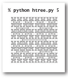
with the additional provisos that the H-trees of order n–1 are halved in size and centered on the four tips of the square. PROGRAM 2.3.4 (htree.py) takes a command-line argument n, and draws an H-tree of order n.
Drawings like these have many practical applications. For example, consider a cable company that needs to run cable to all of the homes distributed throughout its region. A reasonable strategy is to use an H-tree to get the signal to a suitable number of centers distributed throughout the region, then run cables connecting each home to the nearest center. The same problem is faced by computer designers who want to distribute power or signal throughout an integrated circuit chip.
H-trees exhibit exponential growth. An H-tree of order n connects 4n centers, so you would be trying to plot more than 1 million lines with n = 10 and more than 1 billion with n = 15. The program will certainly not finish the drawing with n = 30.
EXERCISE 2.3.14 asks you to modify htree.py to animate the drawing of the H-tree. If you run the resulting program on your computer for a drawing that takes a minute or so to complete, you will, just by watching the drawing progress, have the opportunity to gain substantial insight into the nature of recursive functions, because you can see the order in which the H figures appear and how they form into H-trees. An even more instructive exercise, which derives from the fact that the same drawing results no matter in which order the recursive draw() calls and the stddraw.line() calls appear, is to observe the effect of rearranging the order of these calls on the order in which the lines appear in the emerging drawing (see EXERCISE 2.3.14).

Program 2.3.4 Recursive graphics (htree.py)
import sys
import stddraw
def draw(n, size, x, y):
if n == 0: return
x0 = x - size/2.0
x1 = x + size/2.0
y0 = y - size/2.0
y1 = y + size/2.0
stddraw.line(x0, y, x1, y)
stddraw.line(x0, y0, x0, y1)
stddraw.line(x1, y0, x1, y1)
draw(n-1, size/2.0, x0, y0)
draw(n-1, size/2.0, x0, y1)
draw(n-1, size/2.0, x1, y0)
draw(n-1, size/2.0, x1, y1)
n = int(sys.argv[1])
stddraw.setPenRadius(0.0)
draw(n, 0.5, 0.5, 0.5)
stddraw.show()
n | depth
size | line length
x, y | center
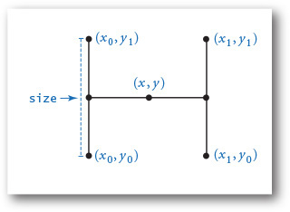
This script accepts a command-line argument n and uses a recursive function to draw an H-tree of order n: it draws three lines in the shape of the letter H that connect the center (x, y) of the square with the centers of the four tips, then calls itself for each of the tips. The integer argument controls the depth of the recursion and the float argument is the size of the initial H.


Brownian bridge
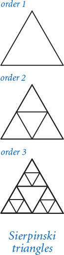
An H-tree is a simple example of a fractal: a geometric shape that can be divided into parts, each of which is (approximately) a reduced-size copy of the original. Fractals are easy to produce with recursive functions, although scientists, mathematicians, and programmers study them from many different points of view. We have already encountered fractals several times in this book—for example, ifs.py (PROGRAM 2.2.4).
The study of fractals plays an important and lasting role in artistic expression, economic analysis, and scientific discovery. Artists and scientists use them to build compact models of complex shapes that arise in nature and resist description using conventional geometry, such as clouds, plants, mountains, riverbeds, human skin, and many others. Economists also use fractals to model function graphs of economic indicators.
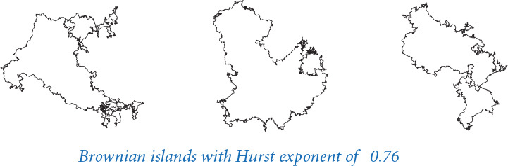
Fractional Brownian motion is a mathematical model for creating realistic fractal models for many naturally rugged shapes. It is used in computational finance and in the study of many natural phenomena, including ocean flows and nerve membranes. Computing the exact fractals specified by the model can be a difficult challenge, but it is not difficult to compute approximations with recursive functions. We consider one simple example here; you can find much more information about the model on the booksite.
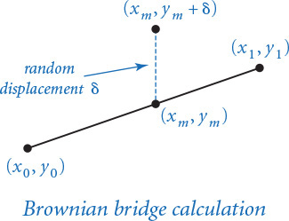
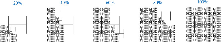
PROGRAM 2.3.5 (brownian.py) plots a function graph that approximates a simple example of fractional Brownian motion known as a Brownian bridge and closely related functions. You can think of this graph as a random walk that connects two points, from (x0, y0) to (x1, y1), controlled by a few parameters. The implementation is based on the midpoint displacement method, which is a recursive plan for drawing the plot within the interval [x0, x1]. The base case is to draw a straight line connecting the two endpoints. The reduction case is to divide the interval into two halves, proceeding as follows:
• Compute the midpoint (xm, ym) of the interval.
• Add to the y-coordinate ym of the midpoint a random value δ, drawn from the Gaussian distribution with mean 0 and a given variance.
• Recur on the subintervals, dividing the variance by a given scaling factor β.
The shape of the curve is controlled by two parameters: the volatility (the initial value of the variance) controls the distance the graph strays from the straight line connecting the points, and the Hurst exponent controls the smoothness of the curve. We denote the Hurst exponent by H and divide the variance by β = 22H at each recursive level. When H is 1/2 (divide by 2 at each level), the curve is a Brownian bridge: a continuous version of the gambler’s ruin problem (see PROGRAM 1.3.8). When 0 < H < 1/2, the displacements tend to increase, resulting in a rougher curve; and when 1/2 < H < 2, the displacements tend to decrease, resulting in a smoother curve. The value 2 –H is known as the fractal dimension of the curve.
Program 2.3.5 Brownian bridge (brownian.py)
import math
import sys
import stddraw
import stdrandom
def curve(x0, y0, x1, y1, var, beta, n=7):
if n == 0:
stddraw.line(x0, y0, x1, y1)
return
xm = (x0 + x1) / 2.0
ym = (y0 + y1) / 2.0
delta = stdrandom.gaussian(0.0, math.sqrt(var))
curve(x0, y0, xm, ym+delta, var/beta, beta, n-1)
curve(xm, ym+delta, x1, y1, var/beta, beta, n-1)
hurstExponent = float(sys.argv[1])
stddraw.setPenRadius(0.0)
beta = 2.0 ** (2.0 * hurstExponent)
curve(0.0, 0.5, 1.0, 0.5, 0.01, beta)
stddraw.show()
n | recursion depth
x0, y0 | left endpoint
x1, y1 | right endpoint
xm, ym | middle
delta | displacement
var | variance
beta | smoothness
This script draws a Brownian bridge across the middle of the window, by adding a small random number (drawn from the Gaussian distribution) to a recursive function that would otherwise plot a straight line. The command-line argument, known as the Hurst exponent, controls the smoothness of the curves—the recursive function uses it to compute a factor beta that adjusts the variance of the Gaussian distribution.

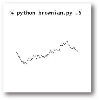
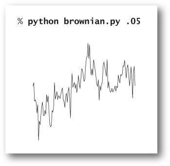
The volatility and initial endpoints of the interval have to do with scale and positioning. The global code in brownian.py allows you to experiment with the smoothness parameter H. With values larger than 1/2, you get plots that look something like the horizon in a mountainous landscape; with values smaller than 1/2, you get plots similar to those you might see for the value of a stock index.
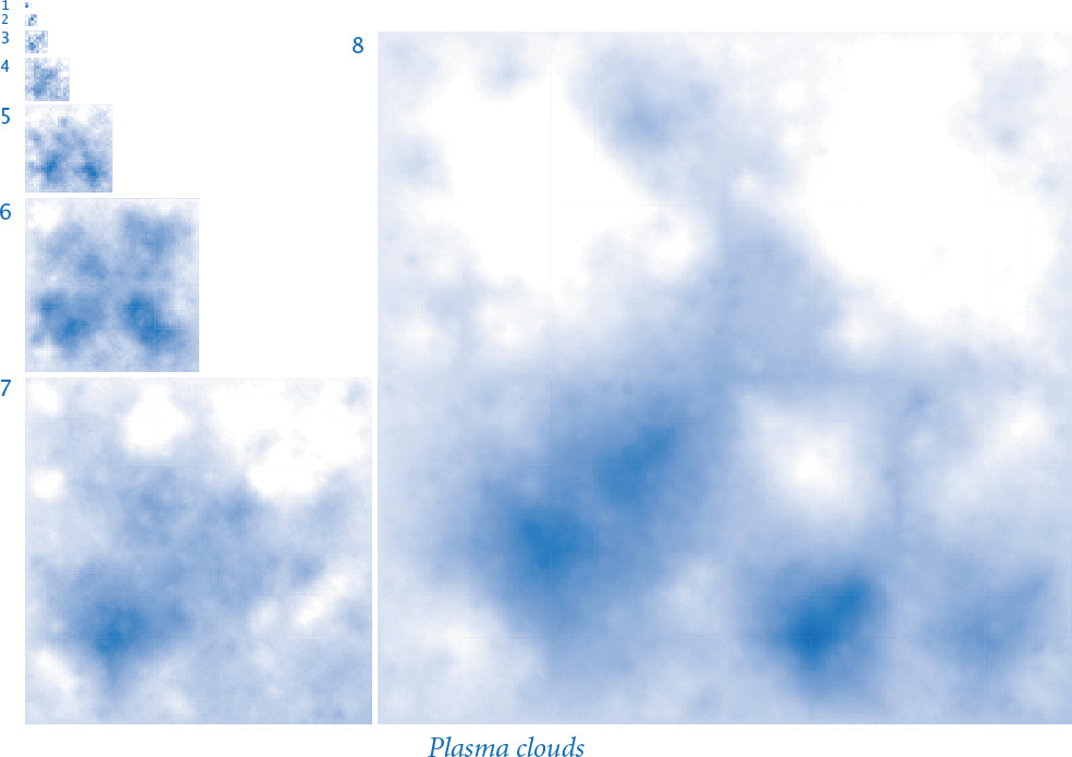
Extending the midpoint displacement method to two dimensions produces fractals known as plasma clouds. To draw a rectangular plasma cloud, we use a recursive plan where the base case is to draw a rectangle of a given color and the reduction step is to draw a plasma cloud in each quadrant with colors that are perturbed from the average with a random number drawn from the Gaussian distribution. Using the same volatility and smoothness controls as in brownian.py, we can produce synthetic clouds that are remarkably realistic. We can use the same code to produce synthetic terrain, by interpreting the color value as the altitude. Variants of this scheme are widely used in the entertainment industry to generate background scenery for movies and computer games.
Pitfalls of recursion
By now, you are perhaps persuaded that recursion can help you compose compact and elegant programs. As you begin to craft your own recursive programs, you need to be aware of several common pitfalls that can arise. We have already discussed one of them in some detail (the running time of your program might grow exponentially). Once identified, these problems are generally not difficult to overcome, but you must be very careful to avoid them when composing recursive functions.
Missing base case
Consider the following recursive function, which is supposed to compute harmonic numbers, but is missing a base case:
def harmonic(n):
return harmonic(n-1) + 1.0/n
If you run a client that calls this function, it will repeatedly call itself and never return, so your program will never terminate. You probably already have encountered infinite loops, where you run your program and nothing happens (or perhaps you get an unending sequence of lines of output). With infinite recursion, however, the result is different because the system keeps track of each recursive call (using a mechanism that we will discuss in SECTION 4.3, based on a data structure known as a stack) and eventually runs out of memory trying to do so. Eventually, Python raises a RuntimeError and reports maximum recursion depth exceeded. When you run a recursive program, you should always try to convince yourself that it has the desired effect by making an informal argument based on mathematical induction. Doing so might uncover a missing base case.
No guarantee of convergence
Another common problem is to include within a recursive function a recursive call to solve a subproblem that is not smaller than the original problem. For example, the following function goes into an infinite recursive loop for any value of its argument n except 1:
def harmonic(n):
if n = 1: return 1.0
return harmonic(n) + 1.0/n
Bugs like this one are easy to spot, but subtle versions of the same problem can be harder to identify.
Excessive memory requirements
If a function calls itself recursively an excessive number of times before returning, the memory required by Python to keep track of the recursive calls may be prohibitive, resulting in a “maximum depth exceeded” run-time error. To get an idea of how much memory is involved, run a small set of experiments using this recursive function for computing the harmonic numbers for increasing values of n (say, by starting at 1,000 and increasing by factors of 10):
def harmonic(n):
if n == 1: return 1.0
return harmonic(n-1) + 1.0/n
The point at which you get the “maximum recursion depth exceeded” run-time error will give you some idea of how much memory Python uses to implement recursion. By contrast, you can run PROGRAM 1.3.5 to compute Hn for huge n using only a tiny bit of space.
Excessive recomputation
The temptation to compose a simple recursive function to solve a problem must always be tempered by the understanding that a simple function might take exponential time (unnecessarily) due to excessive recomputation. This effect is possible even in the simplest recursive functions, and you certainly need to learn to avoid it. For example, the Fibonacci sequence
0, 1, 1, 2, 3, 5, 8, 13, 21, 34, 55, 89, 144, 233, 377, ...
is defined by the recurrence Fn = Fn–1 + Fn–2 for n ≥ 2 with F0 = 0 and F1 = 1. The Fibonacci sequence has many interesting properties and arises in numerous applications. A novice programmer might implement this recursive function to compute numbers in the Fibonacci sequence:
def fib(n):
if n == 0: return 0
if n == 1: return 1
return fib(n-1) + fib(n-2)
This function is spectacularly inefficient—do not use it! Novice programmers often refuse to believe this fact, and run code like this expecting that the computer is certainly fast enough to crank out an answer. Go ahead; see if your computer is fast enough to compute fib(50). To see why it is futile to do so, consider what the function does to compute fib(7) = 13. It first computes fib(6) = 8 and fib(5) = 5. To compute fib(6), it recursively computes fib(5) = 5 again and fib(4) = 3. Things rapidly get worse because both times it computes fib(5), it ignores the fact that it already computed fib(4), and so forth. In fact, you can prove by induction that the number of times this program computes fib(1) when computing fib(n) is precisely Fn (see EXERCISE 2.3.12). The mistake of recomputation is compounded exponentially. As an example, to compute fib(200), the number of times the naive recursive function needs to compute fib(1) is F200 > 1043! No imaginable computer will ever be able to do this many calculations. Beware of programs that might require exponential time. Many calculations that arise and find natural expression as recursive functions fall into this category. Do not fall into the trap of implementing and trying to run them.
The following is one caveat: a systematic technique known as memoization allows us to avoid this pitfall while still taking advantage of the compact recursive description of a computation. In memoization, we maintain an array that keeps track of the values we have computed so that we can return those values and make recursive calls only for new values. This technique is a form of dynamic programming, a well-studied technique for organizing computations that you will learn if you take courses in algorithms or in operations research.

Perspective
Programmers who do not use recursion are missing two opportunities. First, recursion leads to compact solutions to complex problems. Second, recursive solutions embody an argument that the program operates as anticipated. In the early days of computing, the overhead associated with recursive functions was prohibitive in some systems, and many people avoided recursion. In modern systems like Python, recursion is often the method of choice.
If you are intrigued by the mystery of how Python manages to implement the illusion of independently operating copies of the same piece of code, be assured that we will consider this issue in CHAPTER 4. You may be surprised at the simplicity of the solution. It is so easy to implement that programmers were using recursion well before the advent of high-level programming languages like Python. Indeed, you might be surprised to learn that you could compose programs equivalent to the ones considered in this chapter with just the basic loops, conditionals, and arrays programming model discussed in CHAPTER 1.
Recursion has reinforced for us the idea of proving that a program operates as intended. The natural connection between recursion and mathematical induction is essential. For everyday programming, our interest in correctness is to save time and energy tracking down bugs. In modern applications, security and privacy concerns make correctness an essential part of programming. If the programmer cannot be convinced that an application works as intended, how can a user who wants to keep personal data private and secure be so convinced?
Recursive functions truly illustrate the power of a carefully articulated abstraction. While the concept of a function having the ability to call itself seems absurd to many people at first, the many examples that we have considered are certainly evidence that mastering recursion is essential to understanding and exploiting computation and in understanding the role of computational models in studying natural phenomena.
Recursion is the last piece in a programming model that served to build much of the computational infrastructure that was developed as computers emerged to take a central role in daily life in the latter part of the 20th century. Programs built from modules of functions consisting of statements that operate on built-in types of data, conditionals, loops, and function calls (including recursive ones) can solve important applications of all sorts. In the next section, we emphasize this point and review these concepts in the context of a large application. In CHAPTER 3 and CHAPTER 4, we will examine extensions to these basic ideas that embrace the more expansive style of programming that now dominates the computing landscape.
A. No, any loop can be replaced by a recursive function, though the recursive version might require excessive memory.
Q. Are there situations when recursion is the only option available to address a problem?
A. No, any recursive function can be replaced by an iterative counterpart. In SECTION 4.3, we will see how compilers produce code for function calls by using a data structure called a stack.
Q. Which should I prefer, recursion or iteration?
A. Whichever leads to the simpler, more easily understood, or more efficient code.
Q. I get the concern about excessive space and excessive recomputation in recursive code. Anything else to be concerned about?
A. Be extremely wary of creating arrays in recursive code. The amount of space used can pile up very quickly, as can the amount of time required for memory management.
Exercises
2.3.1 What happens if you call factorial() with a negative value of n? With a large value, say, 35?
2.3.2 Write a recursive function that computes the value of ln(n !)
2.3.3 Give the sequence of integers written by a call to ex233(6):
def ex233(n):
if n <= 0: return
stdio.writeln(n)
ex233(n-2)
ex233(n-3)
stdio.writeln(n)
2.3.4 Give the value of ex234(6):
def ex234(n):
if n <= 0: return ''
return ex234(n-3) + str(n) + ex234(n-2) + str(n)
2.3.5 Criticize the following recursive function:
def ex235(n):
s = ex233(n-3) + str(n) + ex235(n-2) + str(n)
if n <= 0: return ''
return s
Solution: The base case will never be reached. A call to ex235(3) will result in calls to ex235(0), ex235(-3), ex235(-6), and so forth until the “maximum depth exceeded” run-time error occurs.
2.3.6 Given four positive integers a, b, c, and d, explain the value computed by gcd(gcd(a, b), gcd(c, d)).
2.3.7 Explain in terms of integers and divisors the effect of the following Euclid-like function:
def gcdlike(p, q):
if q == 0: return p == 1
return gcdlike(q, p % q)
2.3.8 Consider the following recursive function:
def mystery(a, b):
if b == 0:
return 0
if b % 2 == 0:
return mystery(a+a, b/2)
return mystery(a+a, b/2) + a
What are the values of mystery(2, 25) and mystery(3, 11)? Given positive integers a and b, describe the value that mystery(a, b) computes. Answer the same question, but replace + with * and return 0 with return 1.
2.3.9 Write a recursive program rules.py to plot the subdivisions of a ruler using stddraw (see PROGRAM 1.2.1).
2.3.10 Solve the following recurrence relations, all with T(1) = 1. Assume n is a power of 2.
• T(n) = T(n/2) + 1
• T(n) = 2T(n/2) + 1
• T(n) = 2T(n/2) + n
• T(n) = 4T(n/2) + 3
2.3.11 Prove by induction that the minimum possible number of moves needed to solve the towers of Hanoi problem satisfies the same recurrence as the number of moves used by our recursive solution.
2.3.12 Prove by induction that the recursive program given in the text makes exactly Fn recursive calls to fib(1) when computing fib(n).
2.3.13 Prove that the second argument to gcd() decreases by at least a factor of 2 for every second recursive call, and then prove that gcd(p, q) uses at most 2 log2 n + 1 recursive calls where n is the larger of p and q.
2.3.14 Modify htree.py (PROGRAM 2.3.4) to animate the drawing of the H-tree:
Next, rearrange the order of the recursive calls (and the base case), view the resulting animation, and explain each outcome.
Creative Exercises
2.3.15 Binary representation. Compose a program that takes a positive integer n (in decimal) from the command line and writes its binary representation. Recall that in binary.py (PROGRAM 1.3.7, we used the method of subtracting out powers of 2. Instead, use the following simpler method: repeatedly divide 2 into n and read the remainders backward. First, compose a while loop to carry out this computation and write the bits in the wrong order. Then, use recursion to write the bits in the correct order.
2.3.16 A4 paper. The width-to-height ratio of paper in the ISO format is the square root of 2 to 1. Format A0 has an area of 1 square meter. Format A1 is A0 cut with a vertical line into two equal halves, A2 is A1 cut with a horizontal line into in two halves, and so on. Compose a program that takes a command-line integer n and uses stddraw to show how to cut a sheet of A0 paper into 2n pieces.
2.3.17 Permutations. Compose a program permutations.py that takes a command-line argument n and writes all n ! permutations of the n letters starting at a (assuming that n is no greater than 26). A permutation of n elements is one of the n ! possible orderings of the elements. As an example, when n = 3 you should get the following output. Do not worry about in which order you write the permutations.
bca cba cab acb bac abc
2.3.18 Permutations of size k. Modify your solution to the previous exercise so that it takes two command-line arguments n and k, and writes all of the permutations that contain exactly k of the n elements. The number of such permutations is P(n, k) = n ! / (n–k)!. Below is the desired output when k = 2 and n = 4. Do not worry about in which order you enumerate the permutations.
ab ac ad ba bc bd ca cb cd da db dc
2.3.19 Combinations. Compose a program combinations.py that takes one command-line argument n and writes all 2n combinations of any size. A combination is a subset of the n elements, independent of order. As an example, when n = 3 you should get the following output:
a ab abc ac b bc c
Note that your program needs to write the empty string (subset of size 0).
2.3.20 Combinations of size k. Modify your solution to the previous exercise so that it takes two command-line arguments n and k and writes all of the combinations of size k. The number of such combinations is C(n, k) = n ! / (k !(n–k)!). For example, when n = 5 and k = 3, you should get the following output:
abc abd abe acd ace ade bcd bce bde cde
2.3.21 Hamming distance. The Hamming distance between two bit strings of length n is equal to the number of bits in which the two strings differ. Compose a program that takes an integer k and a bitstring s from the command line and writes all bitstrings that have Hamming distance at most k from s. For example, if k is 2 and s is 0000, then your program should write
0011 0101 0110 1001 1010 1100
Hint: Choose k of the n bits in s to flip.
2.3.22 Recursive squares. Compose programs to produce each of the following recursive patterns. The ratio of the sizes of the squares is 2.2:1. To draw a shaded square, draw a filled gray square, then an unfilled black square.

2.3.23 Pancake flipping. You have a stack of n pancakes of varying sizes on a griddle. Your goal is to rearrange the stack in descending order so that the largest pancake is on the bottom and the smallest one is on top. You are only permitted to flip the top k pancakes, thereby reversing their order. Devise a recursive scheme to arrange the pancakes in the proper order that uses at most 2n – 3 flips.
2.3.24 Gray code. Modify beckett.py (PROGRAM 2.3.3) to write the Gray code (not just the sequence of bit positions that change).
2.3.25 Towers of Hanoi variant. Consider the following variant of the towers of Hanoi problem. There are 2n discs of increasing size stored on three poles. Initially all of the discs with odd size (1, 3, ..., 2n-1) are piled on the left pole from top to bottom in increasing order of size; all of the discs with even size (2, 4, ..., 2n) are piled on the right pole. Compose a program to provide instructions for moving the odd discs to the right pole and the even discs to the left pole, obeying the same rules as for towers of Hanoi.
2.3.26 Animated towers of Hanoi. Use stddraw to animate a solution to the towers of Hanoi problem, moving the discs at a rate of approximately 1 per second.
2.3.27 Sierpinski triangles. Compose a recursive program to draw Sierpinski triangles (see PROGRAM 2.2.4). As with htree.py, use a command-line argument to control the depth of the recursion.
2.3.28 Binomial distribution. Estimate the number of recursive calls that would be used by the code
def binomial(n, k):
if (n == 0) or (k == 0): return 1.0
if (n < 0) or (k < 0): return 0.0
return (binomial(n-1, k) + binomial(n-1, k-1)) / 2.0
to compute binomial(100, 50). Develop a better implementation that is based on memoization. Hint: See EXERCISE 1.4.39.
2.3.29 A strange function. Consider McCarthy’s 91 function:
def mcCarthy(n):
if n > 100: return n - 10
return mcCarthy(mcCarthy(n+11))
Determine the value of mcCarthy(50) without using a computer. Give the number of recursive calls used by mcCarthy() to compute this result. Either prove that the base case is reached for all positive integers n or give a value of n for which this function goes into an infinite recursive loop.
2.3.30 Collatz function. Consider the following recursive function, which is related to a famous unsolved problem in number theory, known as the Collatz problem, or the 3n+1 problem:
def collatz(n):
stdio.write(str(n) + ' ')
if n == 1: return
if n % 2 == 0:
collatz(n // 2)
else:
collatz(3*n + 1)
For example, a call to collatz(7) writes this sequence of 17 integers
7 22 11 34 17 52 26 13 40 20 10 5 16 8 4 2 1
after 17 function calls. Compose a program that takes a command-line argument m and returns the value of n < m for which the number of recursive calls for collatz(n) is maximized. The unsolved problem is that no one knows whether the function terminates for all positive values of n (mathematical induction is no help, because one of the recursive calls is for a larger value of the argument). Develop a better implementation that is based on memoization.
2.3.31 Plasma clouds. Compose a program that uses recursion to draw plasma clouds, using the approach suggested in the text.
2.3.32 Recursive tree. Compose a program tree.py that takes a command-line argument n and produces tree-like recursive patterns like these for n equal to 1, 2, 3, 4, and 8:
2.3.33 Brownian island. B. Mandelbrot asked the famous question How long is the coast of Britain? Modify brownian.py (PROGRAM 2.3.5) to get a program brownianisland.py that plots Brownian islands, whose coastlines resemble that of Great Britain. The modifications are simple: first, change curve() to add a Gaussian random variable to the x-coordinate as well as to the y-coordinate; second, change the global code to draw a curve from the point at the center of the canvas back to itself. Experiment with various values of the parameters to get your program to produce islands with a realistic look.
2.4 Case Study: Percolation
The programming tools that we have considered to this point allow us to attack all manner of important problems. We conclude our study of functions and modules by considering a case study of developing a program to solve an interesting scientific problem. Our purpose in doing so is to review the basic elements that we have covered, in the context of the various challenges that you might face in solving a specific problem, and to illustrate a programming style that you can apply broadly.
2.4.2 Vertical percolation detection
2.4.3 Percolation input/output
2.4.5 Percolation probability estimate
Programs in this section
Our example applies a computing technique to a simple model that has been extremely useful in helping scientists and engineers in numerous contexts. We consider a widely applicable technique known as Monte Carlo simulation to study a natural model known as percolation. This is not just of direct importance in materials science and geology, but also explains many other natural phenomena.
The term Monte Carlo simulation is broadly used to encompass any computational technique that employs randomness to estimate an unknown quantity by performing multiple trials (known as simulations). We have used Monte Carlo simulation in several other contexts already—for example, in the gambler’s ruin and coupon collector problems. Rather than develop a complete mathematical model or measure all possible outcomes of an experiment, we rely on the laws of probability and statistics.
You will learn quite a bit about percolation in this case study, but our focus is on the process of developing modular programs to address computational tasks. We identify subtasks that can be addressed independently, striving to identify the key underlying abstractions and asking ourselves questions such as the following: Is there some specific subtask that would help solve this problem? What are the essential characteristics of this specific subtask? Might a solution that addresses these essential characteristics be useful in solving other problems? Asking such questions pays significant dividends, because they lead us to develop software that is easier to create, debug, and reuse, so that we can more quickly address the main problem of interest.
Percolation
It is not unusual for local interactions in a system to imply global properties. For example, an electrical engineer might be interested in composite systems consisting of randomly distributed insulating and metallic materials: which fraction of the materials needs to be metallic so that the composite system is an electrical conductor? As another example, a geologist might be interested in a porous landscape with water on the surface (or oil below); under which conditions will the water be able to drain through to the bottom (or the oil to gush through to the surface)? Scientists have defined an abstract process known as percolation to model such situations. It has been studied widely and shown to be an accurate model in a dizzying variety of applications, beyond insulating materials and porous substances to the spread of forest fires and disease epidemics to evolution to the study of the Internet.
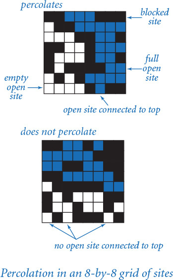
For simplicity, we begin by working in two dimensions and model the system as an n-by-n grid of sites. Each site is either blocked or open; open sites are initially empty. A full site is an open site that can be connected to an open site in the top row via a chain of neighboring (left, right, up, down) open sites. If there is a full site in the bottom row, then we say that the system percolates. In other words, a system percolates if we fill all open sites connected to the top row and that process fills some open site on the bottom row. For the insulating/metallic materials example, the open sites correspond to metallic materials, so that a system that percolates has a metallic path from top to bottom, with full sites conducting. For the porous substance example, the open sites correspond to empty space through which water might flow, so that a system that percolates lets water fill open sites, flowing from top to bottom.
In a famous scientific problem, researchers are interested in the following question: if sites are independently set to be open with vacancy probability p (and therefore blocked with probability 1–p), what is the probability that the system percolates? Despite decades of scientific research, no mathematical solution to this problem has yet been derived. Our task is to compose computer programs to help study the problem.
Basic scaffolding
To address percolation with a Python program, we face numerous decisions and challenges, and we certainly will end up with much more code than in the short programs that we have considered so far in this book. Our goal is to illustrate an incremental style of programming where we independently develop modules that address parts of the problem, building confidence with a small computational infrastructure of our own design and construction as we proceed.
The first step is to pick a representation of the data. This decision will have substantial impact on the kind of code that we compose later, so it is not to be taken lightly. Indeed, it is often the case that we learn something while working with a chosen representation that causes us to scrap it and start all over using a new one.
For percolation, the path to an effective representation is clear: use an n-by-n array. One possibility is to use a code such as 0 to indicate an empty site, 1 to indicate a blocked site, and 2 to indicate a full site. Alternatively, note that we typically describe sites in terms of questions: Is the site open or blocked? Is the site full or empty? This characteristic of the elements suggests that we might use an n-by-n array in which each element is either True or False. In computer science, we refer to such two-dimensional arrays as boolean matrices.
Boolean matrices are fundamental mathematical objects with many applications. Python does not provide direct support for operations on boolean matrices, but we can use the functions in stdarray to read and write boolean matrices. This choice illustrates a basic principle that often comes up in programming: the effort required to build a more general tool usually pays dividends. Using a natural abstraction such as boolean matrices is preferable to using a specialized representation. In the present context, it turns out that using boolean matrices instead of integer matrices leads to code that is easier to understand.
Eventually, we will want to work with random data, but we also want to be able to read and write files because debugging programs with random inputs can be counterproductive. With random data, you get a different input each time that you run the program; after fixing a bug, what you want to see is the same input that you just used, to check that the fix was effective. Accordingly, it is best to start with some specific cases that we understand, kept in files formatted to be read by stdarray.readBool2D() (dimensions followed by 0 and 1 values in row-major order).
When you start working on a new problem that involves several files, it is usually worthwhile to create a new folder (directory) to isolate those files from others that you may be working on. For example, we might create a folder named percolation to store the code we compose in this section. We can then implement and debug the basic code for reading and writing percolation systems, create test files, check that the files are compatible with the code, and so forth, before really worrying about percolation at all. This type of code, sometimes called scaffolding, is straightforward to implement, but making sure that it is solid at the outset will save us from distraction when approaching the main problem.
Now we can turn to the code for testing whether a boolean matrix represents a system that percolates. Referring to the helpful interpretation in which we can think of the task as simulating what would happen if the top were flooded with water (does it flow to the bottom or not?), our first design decision is that we will want to have a flow() function that takes as an argument a boolean matrix isOpen[][] that specifies which sites are open and returns another boolean matrix isFull[][] that specifies which sites are full. For the moment, we will not worry at all about how to implement this function; we are just deciding how to organize the computation. It is also clear that we will want client code to be able to use a percolates() function that checks whether the boolean matrix returned by flow() has any full sites on the bottom.
PROGRAM 2.4.1 (percolation0.py) summarizes these decisions. It does not perform any interesting computation, but, after running and debugging this code we can start thinking about actually solving the problem. A function that performs no computation, such as flow(), is sometimes called a stub. Having this stub allows us to test and debug percolates() and main() in the context in which we will need them. We refer to code like PROGRAM 2.4.1 as scaffolding. As with the scaffolding that construction workers use when erecting a building, this kind of code provides the support that we need to develop a program. By fully implementing and debugging this code (much, if not all, of which we need, anyway) at the outset, we provide a sound basis for building code to solve the problem at hand. Often, we carry the analogy one step further and remove the scaffolding (or replace it with something better) after the implementation is complete.
Vertical percolation
Given a boolean matrix that represents the open sites, how do we figure out whether it represents a system that percolates? As we will see at the end of this section, this computation turns out to be directly related to a fundamental question in computer science. For the moment, we will consider a much simpler version of the problem that we call vertical percolation.
Program 2.4.1 Percolation scaffolding (percolation0.py)
import stdarray
import stdio
def flow(isOpen):
n = len(isOpen)
isFull = stdarray.create2D(n, n, False)
# Percolation flow computation goes here.
# See Program 2.4.2 and Program 2.4.6.
return isFull
def percolates(isOpen):
isFull = flow(isOpen)
n = len(isFull)
for j in range(n):
if isFull[n-1][j]: return True
return False
def main():
isOpen = stdarray.readBool2D()
stdarray.write2D(flow(isOpen))
stdio.writeln(percolates(isOpen))
if __name__ == '__main__': main()
n | system size (n-by-n)
isFull[][] | full sites
isOpen[][] | open sites
To get started with percolation, we compose this code, which handles all the straightforward tasks surrounding the computation. The primary function flow() returns a two-dimensional array giving the full sites (none, in the placeholder code here). The helper function percolates() checks the bottom row of the returned array to decide whether the system percolates. The test client reads a boolean two-dimensional array from standard input and then writes the result of calling flow() and percolates() for that array.
% more test5.txt
5 5
0 1 1 0 1
0 0 1 1 1
1 1 0 1 1
1 0 0 0 1
0 1 1 1 1
% python percolation0.py < test5.txt
5 5
0 0 0 0 0
0 0 0 0 0
0 0 0 0 0
0 0 0 0 0
0 0 0 0 0
False
The simplification is to restrict attention to vertical connection paths. If such a path connects top to bottom in a system, we say that the system vertically percolates along the path (and that the system itself vertically percolates). This restriction is perhaps intuitive if we are talking about sand traveling through cement, but not if we are talking about water traveling through cement or about electrical conductivity. Simple as it is, vertical percolation is a problem that is interesting in its own right because it suggests various mathematical questions. Does the restriction make a significant difference? How many vertical percolation paths do we expect?
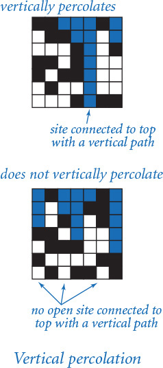
Determining the sites that are filled by some path that is connected vertically to the top is a simple calculation. We initialize the top row of our result array from the top row of the percolation system, with full sites corresponding to open ones. Then, moving from top to bottom, we fill in each row of the array by checking the corresponding row of the percolation system. Proceeding from top to bottom, we fill in the rows of isFull[][] to mark as True all elements that correspond to sites in isOpen[][] that are vertically connected to a full site on the previous row. PROGRAM 2.4.2 (percolationv.py) is the same as percolation0.py except for an implementation of flow() that returns a boolean matrix of full sites (True if connected to the top via a vertical path, False otherwise).
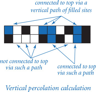
Testing
After we become convinced that our code is behaving as planned, we want to run it on a broader variety of test cases and address some of our scientific questions. At this point, our initial scaffolding becomes less useful, as representing large boolean matrices with 0s and 1s on standard input and standard output and maintaining large numbers of test cases quickly becomes uninformative and unwieldy. Instead, we want to automatically generate test cases and observe the operation of our code on them, to be sure that it is operating as expected. Specifically, to gain confidence in our code and to develop a better understanding of percolation, our next goals are to:
• Test our code for large random boolean matrices.
• Given a vacancy probability p, estimate the system percolation probability.
Program 2.4.2 Vertical percolation detection (percolationv.py)
# Same as percolation0.py except replace flow() with this:
def flow(isOpen):
n = len(isOpen)
isFull = stdarray.create2D(n, n, False)
for j in range(n):
isFull[0][j] = isOpen[0][j]
for i in range(1, n):
for j in range(n):
if isOpen[i][j] and isFull[i-1][j]:
isFull[i][j] = True
return isFull
n | system size (n-by-n)
isFull[][] | full sites
isOpen[][] | open sites
Substituting this function for the stub in PROGRAM 2.4.2 gives a solution to the vertical-only percolation problem that solves our test case as expected (see text).
% more test5.txt
5 5
0 1 1 0 1
0 0 1 1 1
1 1 0 1 1
1 0 0 0 1
0 1 1 1 1
% python percolationv.py < test5.txt
5 5
0 1 1 0 1
0 0 1 0 1
0 0 0 0 1
0 0 0 0 1
0 0 0 0 1
True
To accomplish these goals, we need new clients that are slightly more sophisticated than the scaffolding we used to get the program up and running. Our modular programming style is to develop such clients in independent modules without modifying our percolation code at all.
Monte Carlo simulation
We want our code to work properly for any boolean matrix. Moreover, the scientific question of interest involves random boolean matrices. To this end, we compose a function random() that takes two arguments n and p and generates a random n-by-n boolean array in which the probability that each element is True is p. Having debugged our code on a few specific test cases, we can use this function to test it on larger random systems. It is possible that such cases may uncover a few more bugs, so some care is in order to check results. However, having debugged our code for a small system, we can proceed with some confidence. It is easier to focus on new bugs after eliminating the obvious bugs.
Data visualization
We can work more easily with bigger problem instances if we use stddraw for output. Accordingly, we develop a function draw() to visualize the contents of a boolean matrix as a subdivision of the standard drawing window into squares, one for each site. For flexibility, we include a second argument that specifies which squares we want to fill—those corresponding to True elements or those corresponding to False elements. As you will see, this function pays dividends in its ability to help us visualize large problem instances. Using draw() to draw our arrays representing blocked and full sites in different colors gives a compelling visual representation of percolation.
With these tools, testing our percolation code for larger boolean matrices on a larger set of trials is straightforward. PROGRAM 2.4.3 (percolationio.py) is a small module that contains the two functions just described, for use as input and output for testing our percolation code; PROGRAM 2.4.4 (visualizev.py) is a client script that takes a percolation system size, a probability, and a number of trials from the command line and then runs the specified number of trials, creating a new random boolean matrix, and displaying the result of the percolation flow calculation for each, pausing for a brief time between trials.
Our eventual goal is to compute an accurate estimate of percolation probabilities, perhaps by running a large number of trials. Nevertheless, these tools helps us gain more familiarity with the problem by studying some large cases (while at the same time gaining confidence that our code is working properly). When you run visualizev.py for moderate-size n (50 to 100, say) and various values of p, you will immediately be drawn into using this program to try to answer some questions about percolation. Clearly, the system never percolates when p is low and always percolates when p is very high. How does it behave for intermediate values of p? How does the behavior change as n increases?
Program 2.4.3 Percolation input/output (percolationio.py)
import sys
import stdarray
import stddraw
import stdio
import stdrandom
def random(n, p):
a = stdarray.create2D(n, n, False)
for i in range(n):
for j in range(n):
a[i][j] = stdrandom.bernoulli(p)
return a
def draw(a, which):
n = len(a)
stddraw.setXscale(-1, n)
stddraw.setYscale(-1, n)
for i in range(n):
for j in range(n):
if a[i][j] == which:
stddraw.filledSquare(j, n-i-1, 0.5)
def main():
n = int(sys.argv[1])
p = float(sys.argv[2])
test = random(n, p)
draw(test, False)
stddraw.show()
if __name__ == '__main__': main()
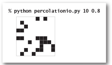
These helper functions are useful for testing when we are studying percolation. The call random(n, p) creates a random n-by-n boolean array, where the probability that each element is True is p, and the call draw(test, False) produces a visualization of the given two-dimensional array in the standard drawing window, with filled squares corresponding to False elements.
Program 2.4.4 Visualization client (visualizev.py)
import sys
import stddraw
import percolationv
import percolationio
n = int(sys.argv[1])
p = float(sys.argv[2])
trials = int(sys.argv[3])
for i in range(trials):
isOpen = percolationio.random(n, p)
stddraw.clear()
stddraw.setPenColor(stddraw.BLACK)
percolationio.draw(isOpen, False)
stddraw.setPenColor(stddraw.BLUE)
isFull = percolationv.flow(isOpen)
percolationio.draw(isFull, True)
stddraw.show(1000.0)
stddraw.show()
n | system size (n-by-n)
p | site vacancy probability
trials | number of trials
isOpen[][] | open sites
isFull[][] | full sites
This client takes command-line arguments n, p, and trials, then generates random n-by-n boolean arrays with site vacancy probability p, computes the directed percolation flow, and draws the result in the stanard drawing window. Such drawings increase confidence that our code is operating properly and help develop an intuitive understanding of percolation.

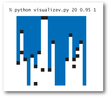
Estimating probabilities
The next step in our program development process is to compose code to estimate the probability that a random system percolates. We refer to this quantity as the percolation probability. To estimate its value, we simply run a number of experiments. The situation is no different from our study of coin flipping (see PROGRAM 2.2.7), but instead of flipping a coin, we generate a random system and check whether it percolates.
PROGRAM 2.4.5 (estimatev.py) encapsulates this computation in a function evaluate() that returns an estimate of the probability that an n-by-n system with site vacancy probability p percolates, obtained by generating a given number of random systems and calculating the fraction of them that percolate. The function takes three arguments: n, p, and trials.
How many trials do we need to obtain an accurate estimate of the percolation probability? This question is addressed by basic methods in probability and statistics, which are beyond the scope of this book, but we can get a feeling for the problem with computational experience. With just a few runs of estimatev.py, you can learn that if the site vacancy probability is close to 0 or very close to 1, then we do not need many trials, but that there are values for which we need as many as 10,000 trials to be able to estimate the percolation probability within two decimal places. To study the situation in more detail, we might modify estimatev.py to produce output like bernoulli.py (PROGRAM 2.2.7), plotting a histogram of the data points so that we can see the distribution of values (see EXERCISE 2.4.11).
Using estimatev.evaluate() represents a giant leap in the amount of computation that we are doing. All of a sudden, it makes sense to run thousands of trials. It would be unwise to try to do so without first having thoroughly debugged our percolation functions. Also, we need to begin to take the time required to complete the computation into account. The basic methodology for doing so is the topic of SECTION 4.1, but the structure of these programs is sufficiently simple that we can do a quick calculation, which we can verify by running the program. Each trial involves n2 sites, so the total running time of estimatev.evaluate() is proportional to n2 times the number of trials. If we increase the number of trials by a factor of 10 (to gain more precision), the running time increases by about a factor of 10. If we increase n by a factor of 10 (to study percolation for larger systems), the running time increases by about a factor of 100.
Can we run this program to determine percolation probabilities for a system with billions of sites with several digits of precision? No. No computer is fast enough to use estimatev.evaluate() for this purpose. Moreover, in a scientific experiment on percolation, the value of n is likely to be much higher. We can hope to formulate a hypothesis from our simulation that can be tested experimentally on a much larger system, but not to precisely simulate a system that corresponds atom-for-atom with the real world. Simplification of this sort is essential in science.
Program 2.4.5 Percolation probability estimate (estimatev.py)
import sys
import stdio
import percolationv
import percolationio
def evaluate(n, p, trials):
count = 0
for i in range(trials):
isOpen = percolationio.random(n, p)
if (percolationv.percolates(isOpen)):
count += 1
return 1.0 * count / trials
def main():
n = int(sys.argv[1])
p = float(sys.argv[2])
trials = int(sys.argv[3])
q = evaluate(n, p, trials)
stdio.writeln(q)
if __name__ == '__main__': main()
n | system size (n-by-n)
p | site vacancy probability
trials | number of trials
isOpen[][] | open sites
q | percolation probability
To estimate the probability that a system percolates, we generate random n-by-n systems with site vacancy probability p and compute the fraction of them that percolate. This is a Bernoulli process, no different from coin flipping (see PROGRAM 2.2.6). Increasing the number of trials increases the accuracy of the estimate. If the site vacancy probability is close to 0 or to 1, not many trials are needed.
% python estimatev.py 20 .75 10
0.0
% python estimatev.py 20 .95 10
1.0
% python estimatev.py 20 .85 10
0.7
% python estimatev.py 20 .85 1000
0.564
% python estimatev.py 20 .85 1000
0.561
% python estimatev.py 40 .85 100
0.11
You are encouraged to download estimatev.py from the booksite to get a feel for both the percolation probabilities and the amount of time required to compute them. When you do so, you are not just learning more about percolation, but also testing the hypothesis that the models we have described apply to the running times of our simulations of the percolation process.
What is the probability that a system with site vacancy probability p vertically percolates? Vertical percolation is sufficiently simple that elementary probabilistic models can yield an exact formula for this quantity, which we can validate experimentally with estimatev.py. Since our only reason for studying vertical percolation was that it represented an easy starting point around which we could develop supporting software for studying percolation methods, we leave further study of vertical percolation for an exercise (see EXERCISE 2.4.13) and turn to the main problem.
Recursive solution for percolation
How do we test whether a system percolates in the general case when any path starting at the top and ending at the bottom (not just a vertical one) will do the job?
Remarkably, we can solve this problem with a compact program, based on a classic recursive scheme known as depth-first search. PROGRAM 2.4.6 (percolation.py) is an implementation of flow() that computes the flow matrix isFull[][], based on a recursive four-argument function _flow(). The recursive function takes as arguments the site vacancy matrix isOpen[][], the flow matrix isFull[][], and a site position specified by a row index i and a column index j. The base case is a recursive call that just returns (we refer to such a call as a null call), for one of the following reasons:
• Either i or j is outside the two-dimensional array bounds.
• The site is blocked (isOpen[i][j] is False).
• We have already marked the site as full (isFull[i][j] is True).
The reduction case is to mark the site as filled and issue recursive calls for the site’s four neighbors: isOpen[i+1][j], isOpen[i][j+1], isOpen[i][j-1], and isOpen[i-1][j]. To implement flow(), we call the recursive _flow() function for every site on the top row. The recursion always terminates because each recursive call either is null or marks a new site as full. We can show by an induction-based argument (as usual for recursive programs) that a site is marked as full if and only if it is open and connected to one of the sites on the top row via a chain of neighboring open sites.
Program 2.4.6 Percolation detection (percolation.py)
# Same as percolation0.py except replace flow() with this code:
def _flow(isOpen, isFull, i, j):
n = len(isFull)
if (i < 0) or (i >= n): return
if (j < 0) or (j >= n): return
if not isOpen[i][j]: return
if isFull[i][j]: return
isFull[i][j] = True
_flow(isOpen, isFull, i+1, j ) # Down.
_flow(isOpen, isFull, i , j+1) # Right.
_flow(isOpen, isFull, i , j-1) # Left.
_flow(isOpen, isFull, i-1, j ) # Up.
def flow(isOpen):
n = len(isOpen)
isFull = stdarray.create2D(n, n, False)
for j in range(n):
_flow(isOpen, isFull, 0, j)
return isFull
n | system size (n-by-n)
isOpen[][] | open sites
isFull[][] | full sites
i, j | current site row, column
Substituting these functions for the flow() stub in PROGRAM 2.4.1 gives a depth-first-search-based solution to the percolation problem. The call _flow(isOpen, isFull, i, j) fills sites by setting to True the element in isFull[][] corresponding to any site that can be reached from isOpen[i][j] via a path of open sites. The one-argument flow() calls the recursive function for every site on the top row.
% more test8.txt
8 8
0 0 1 1 1 0 0 0
1 0 0 1 1 1 1 1
1 1 1 0 0 1 1 0
0 0 1 1 0 1 1 1
0 1 1 1 0 1 1 0
0 1 0 0 0 0 1 1
1 0 1 0 1 1 1 1
1 1 1 1 0 1 0 0
% python percolation.py < test8.txt
8 8
0 0 1 1 1 0 0 0
0 0 0 1 1 1 1 1
0 0 0 0 0 1 1 0
0 0 0 0 0 1 1 1
0 0 0 0 0 1 1 0
0 0 0 0 0 0 1 1
0 0 0 0 1 1 1 1
0 0 0 0 0 1 0 0
True
Tracing the operation of _flow() on a tiny test case is an instructive exercise in examining the dynamics of the process, as shown in the diagram at left. The function calls itself for every site that can be reached via a path of open sites from the top. This example illustrates that simple recursive programs can mask computations that otherwise are quite sophisticated. This function is a special case of the classic depth-first search algorithm, which has many important applications.
We can visualize and perform experiments with this algorithm using scripts like the visualizev.py and estimatev.py tools that we have developed. To do so, we can create the file visualize.py as a copy of visualizev.py, and then edit visualize.py by replacing the two instances of percolationv with percolation. Similarly, we can create the file estimate.py as an edited copy of estimatev.py. (To save space, we do not show visualize.py and estimate.py in the book; they are available through the booksite.) If you do so, and try various values for n and p, you will quickly get a feeling for the situation: the systems always percolate when p is high and never percolate when p is low, and (particularly as n increases) there is a value of p above which the systems (almost) always percolate and below which they (almost) never percolate (see examples at the top of the next page).
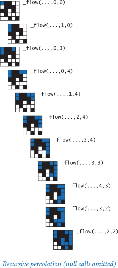
Having debugged visualizev.py and estimatev.py on the simple vertical percolation process, we can use them with more confidence to study percolation, and turn quickly to study the real scientific problem of interest. Note that if we want to study both versions of percolation, we could compose clients of both percolationv and percolation that call both flow() functions to compare them.
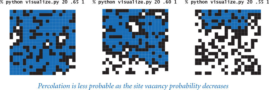
Adaptive plot
To gain more insight into percolation, our next step in program development might be to compose a program that plots the percolation probability q as a function of the site vacancy probability p for a given value of n. Perhaps the best way to produce such a plot is to first derive a mathematical equation for the function, and then use that equation to make the plot. For percolation, however, no one has been able to derive such an equation, so the next option is to use the Monte Carlo method: run simulations and plot the results.
Immediately, we are faced with numerous decisions. For how many values of p should we compute an estimate of the percolation probability? Which values of p should we choose? How much precision should we aim for in these calculations? These decisions constitute an experimental design problem. Much as we might like to instantly produce an accurate rendition of the curve for any given n, the computation cost can be prohibitive. For example, the first thing that comes to mind is to plot, say, 100 to 1,000 equally spaced points, using stdstats.py (PROGRAM 2.2.5). But, as you learned from using estimate.py, computing a sufficiently precise value of the percolation probability for each point might take several seconds or longer, so the whole plot might take minutes or hours or even longer. Moreover, it is clear that a lot of this computation time is completely wasted, because we know that values for small p are 0 and values for large p are 1. We might prefer to spend that time on more precise computations for intermediate p. How should we proceed?
PROGRAM 2.4.7 (percplot.py) implements a recursive approach that is widely applicable to similar problems. The basic idea is simple: we choose the minimum distance that we want between values of the x-coordinate (which we refer to as the gap tolerance), the minimum known error that we wish to tolerate in the y-coordinate (which we refer to as the error tolerance), and the number of trials per point that we wish to perform. The recursive function draws the plot within a given x-interval [x0, x1], from (x0, y0) to (x1, y1). For our problem, the plot is from (0, 0) to (1, 1). The base case (if the distance between x0 and x1 is less than the gap tolerance, or the distance between the line connecting the two endpoints and the value of the function at the midpoint is less than the error tolerance) is to simply draw a line from (x0, y0) to (x1, y1). The reduction step is to (recursively) plot the two halves of the curve, from (x0, y0) to (xm, ym) and from (xm, ym) to (x1, y1).
Program 2.4.7 Adaptive plot client (percplot.py)
import sys
import stddraw
import estimate
def curve(n, x0, y0, x1, y1, trials=10000, gap=0.01, err=0.0025):
xm = (x0 + x1) / 2.0
ym = (y0 + y1) / 2.0
fxm = estimate.evaluate(n, xm, trials)
if (x1 - x0 < gap) or (abs(ym - fxm) < err):
stddraw.line(x0, y0, x1, y1)
stddraw.show(0.0)
return
curve(n, x0, y0, xm, fxm)
stddraw.filledCircle(xm, fxm, 0.005)
stddraw.show(0.0)
curve(n, xm, fxm, x1, y1)
n = int(sys.argv[1])
stddraw.setPenRadius(0.0)
curve(n, 0.0, 0.0, 1.0, 1.0)
stddraw.show()
n | system size (n-by-n)
x0, y0 | left endpoint
x1, y1 | right endpoint
xm, ym | midpoint
fxm | value at midpoint
trials | number of trials
gap | gap tolerance
err | error tolerance
This program accepts an integer n as a command-line argument and then runs experiments to build an adaptive plot that relates site vacancy probability (the control variable) to percolation probability (the experimental observations) for n-by-n systems.
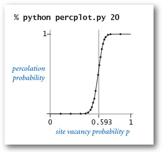

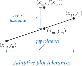
The code in percplot.py is relatively simple and produces a good-looking curve at relatively low cost. We can use it to study the shape of the curve for various values of n, or we can choose smaller tolerances to be more confident that the curve is close to the actual values. Precise mathematical statements about quality of approximation can, in principle, be derived, but it is perhaps not appropriate to go into too much detail while exploring and experimenting, since our goal is simply to develop a hypothesis about percolation that can be tested by scientific experimentation.
Indeed, the curves produced by percplot.py immediately confirm the hypothesis that there is a threshold value (about 0.593): if p is greater than the threshold, then the system almost certainly percolates; if p is less than the threshold, then the system almost certainly does not percolate. As n increases, the curve approaches a step function that changes value from 0 to 1 at the threshold. This phenomenon, known as a phase transition, is found in many physical systems.

The simple form of the output of percplot.py masks the huge amount of computation behind it. For example, the curve drawn for n = 100 has 18 points, each the result of 10,000 trials, each trial involving n2 sites. Generating and testing each site involves a few lines of code, so this plot comes at the cost of executing billions of statements. There are two lessons to be learned from this observation. First, we need to have confidence in any line of code that might be executed billions of times, so our care in developing and debugging code incrementally is justified. Second, although we might be interested in systems that are much larger, we need further study in computer science to be able to handle larger cases—that is, to develop faster algorithms and a framework for knowing their performance characteristics.
With this reuse of all of our software, we can study all sorts of variants on the percolation problem, just by implementing different flow() functions. For example, if you leave out the last recursive call in the recursive _flow() function in PROGRAM 2.4.6, it tests for a type of percolation known as directed percolation, where paths that go up are not considered. This model might be important for a situation like a liquid percolating through porous rock, where gravity might play a role, but not for a situation like electrical connectivity. If you run percplot.py for both functions, will you be able to discern the difference (see EXERCISE 2.4.5)?
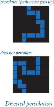
To model physical situations such as water flowing through porous substances, we need to use three-dimensional arrays. Is there a similar threshold in the three-dimensional problem? If so, what is its value? Depth-first search is effective for studying this question, though the addition of another dimension requires that we pay even more attention to the computational cost of determining whether a system percolates (see EXERCISE 2.4.21). Scientists also study more complex lattice structures that are not well modeled by multidimensional arrays—we will see how to model such structures in SECTION 4.5.
Percolation is interesting to study via in silico experimentation because no one has been able to derive the threshold value mathematically for several natural models. The only way that scientists know the value is by using Monte Carlo simulations like those we have studied in this section. A scientist needs to do experiments to see whether the percolation model reflects what is observed in nature, perhaps through refining the model (for example, using a different lattice structure). Percolation is an example of an increasing number of problems where computer science of the kind described here is an essential part of the scientific process.
Lessons
We might have approached the problem of studying percolation by sitting down to design and implement a single program, which probably would run to hundreds of lines, to produce the kind of plots that are drawn by PROGRAM 2.4.7. In the early days of computing, programmers had little choice but to work with such programs, and would spend enormous amounts of time isolating bugs and correcting design decisions. With modern programming tools like Python, we can do better, using the incremental modular style of programming presented in this chapter and keeping in mind some of the lessons that we have learned.
Expect bugs
Every interesting piece of code that you compose will have at least one or two bugs, if not many more. By running small pieces of code on small test cases that you understand, you can more easily isolate any bugs and then more easily fix them when you find them. Once the code is debugged, you can depend on using a module as a building block for any client.
Keep modules small
You can focus attention on at most a few dozen lines of code at a time, so you may as well break your code into small modules as you compose it. Some modules that contain collections of related functions may eventually grow to contain hundreds of lines of code; otherwise, we should work with small files.

Limit interactions
In a well-designed modular program, most modules should depend on just a few others. In particular, a module that calls a large number of other modules needs to be divided into smaller pieces. Modules that are called by a large number of other modules (you should have only a few) need special attention, because if you do need to make changes in a module’s API, you have to reflect those changes in all its clients.
Develop code incrementally
You should run and debug each small module as you implement it. That way, you are never working with more than a few dozen lines of unreliable code at any given time. If you put all your code in one big module, it is difficult to be confident that any of it is safe from bugs. Running code early also forces you to think sooner rather than later about I/O formats, the nature of problem instances, and other issues. Experience gained when thinking about such issues and debugging related code makes the code that you develop later in the process more effective.
Solve an easier problem
Some working solution is better than no solution, so it is typical to begin by putting together the simplest code that you can craft that solves a given problem, as we did with vertical-only percolation. This implementation is the first step in a process of continual refinements and improvements as we develop a more complete understanding of the problem by examining a broader variety of test cases and developing support software such as our visualize.py and estimate.py programs.
Consider a recursive solution
Recursion is an indispensable tool in modern programming that you should learn to trust. If you are not already convinced of this fact by the simplicity and elegance of percplot.py and percolation.py, you might wish to try to develop a nonrecursive program for testing whether a system percolates and then reconsider the issue.
Build tools when appropriate
Our visualization function draw() and random boolean matrix generation function random() of percolationio.py are certainly useful for many other applications, as is the adaptive plotting function curve() of percplot.py. Incorporating these functions into appropriate modules would be simple. It is no more difficult (indeed, perhaps easier) to implement general-purpose functions like these than it would be to implement special-purpose functions for percolation.
Reuse software when possible
Our stdio, stdrandom, and stddraw modules all simplified the process of developing the code in this section, and we were also immediately able to reuse programs such as estimate.py, and visualize.py for percolation after developing them for vertical percolation. After you have composed a few programs of this kind, you might find yourself developing versions of these programs that you can reuse for other Monte Carlo simulations or other experimental data analysis problems.
The primary purpose of this case study is to convince you that modular programming will take you much further than you could get without it. Although no approach to programming is a panacea for all problems, the tools and approach that we have discussed in this section will allow you to attack complex programming tasks that might otherwise be far beyond your reach.
The success of modular programming is only a start. Modern programming systems rely on a vastly more flexible programming model than the module-as-a-collection-of-functions model that we have been considering. In the next two chapters, we develop this model, along with many examples that illustrate its utility.
Q&A
Q. Editing visualize.py and estimate.py to rename every occurrence of percolation to percolationv (or whatever module we want to study) seems to be a bother. Is there a way to avoid doing so?
A. Yes. The most straightforward approach is to keep multiple files named percolation.py in separate subdirectories. Then copy the desired percolation.py file from one of the subdirectories to your working directory, thereby selecting one particular implementation. An alternative approach is to use Python’s import as statement to define an identifier to refer to the module:
import percolationv as percolation
Now, any call to percolation.percolates() uses the function defined in percolationv.py instead of the one defined in percolation.py. In this situation, changing implementations involves editing only one line of source code.
Q. That recursive flow() function makes me nervous. How can I better understand what it’s doing?
A. Run it for small examples of your own making, instrumented with instructions to write a function-call trace. After a few runs, you will gain confidence that it always fills the sites connected to the start point.
Q. Is there a simple nonrecursive approach?
A. There are several known approaches that perform the same basic computation. We will revisit the problem at the end of the book, in SECTION 4.5. In the meantime, working on developing a nonrecursive implementation of flow() is certain to be an instructive exercise, if you are interested.
Q. PROGRAM 2.4.7 (percplot.py) seems to involve a huge amount of calculation to get a simple function graph. Is there some better way?
A. The best strategy would be a mathematical proof of the threshold value, but that derivation has eluded scientists.
Exercises
2.4.1 Compose a program that takes a command-line argument n and creates an n-by-n boolean array with the element in row i and column j set to True if i and j are relatively prime, then shows the n-by-n boolean array on standard drawing (see EXERCISE 1.4.14). Then, compose a similar program to draw the Hadamard matrix of order n (see EXERCISE 1.4.27) and another program to draw the matrix with the element in row n and column j set to True if the coefficient of xj in (1+x)i (binomial coefficient) is odd (see EXERCISE 1.4.39). You may be surprised at the pattern formed by the latter.
2.4.2 Compose a write() function for percolationIO.py that writes 1 for blocked sites, 0 for open sites, and * for full sites.
2.4.3 Give the recursive calls for percolation.py given the following input:
3 3
1 0 1
0 0 0
1 1 0
2.4.4 Compose a client of percolation.py like visualize.py that does a series of experiments for a command-line argument n where the site vacancy probability p increases from 0 to 1 by a given increment (also taken from the command line).
2.4.5 Compose a program percolationd.py that tests for directed percolation (by leaving off the last recursive call in the recursive _flow() function in PROGRAM 2.4.6, as described in the text), then use percplot.py (suitably modified) to draw a plot of the directed percolation probability as a function of the site vacancy probability.
2.4.6 Compose a client of percolation.py and percolationd.py that takes a site vacancy probability p from the command line and writes an estimate of the probability that a system percolates but does not percolate down. Perform enough experiments to get an estimate that is accurate to three decimal places.
2.4.7 Describe the order in which the sites are marked when percolation.py is used on a system with no blocked sites. Which is the last site marked? What is the depth of the recursion?
2.4.8 Modify percolation.py to animate the flow computation, showing the sites filling one by one. Check your answer to the previous exercise.
2.4.9 Experiment with using percplot.py to plot various mathematical functions (just by replacing the call on estimate.evaluate() with an expression that evaluates the function). Try the function sin(x) + cos(10*x) to see how the plot adapts to an oscillating curve, and come up with interesting plots for three or four functions of your own choosing.
2.4.10 Modify percolation.py to compute the maximum depth of the recursion used in the flow calculation. Plot the expected value of that quantity as a function of the site vacancy probability p. How does your answer change if the order of the recursive calls is reversed?
2.4.11 Modify estimate.py to produce output like that produced by bernoulli.py (PROGRAM 2.2.7). Extra credit: Use your program to validate the hypothesis that the data obeys the Gaussian (normal) distribution.
2.4.12 Modify percolationio.py, estimate.py, percolation.py, and visualize.py to handle m-by-n grids and m-by-n boolean matrices. Use an optional argument so that m defaults to n if only one of the two dimensions is specified.
Creative Exercises
2.4.13 Vertical percolation. Show that an n-by-n percolation system with site vacancy probability p vertically percolates with probability 1 – (1 – pn)n, and use estimate.py to validate your analysis for various values of n.
2.4.14 Rectangular percolation systems. Modify the code in this section to allow you to study percolation in rectangular systems. Compare the percolation probability plots of systems whose ratio of width to height is 2:1 with those whose ratio is 1:2.
2.4.15 Adaptive plotting. Modify percplot.py to take its control parameters (gap tolerance, error tolerance, and number of trials) from the command line. Experiment with various values of the parameters to learn their effect on the quality of the curve and the cost of computing it. Briefly describe your findings.
2.4.16 Percolation threshold. Compose a percolation.py client that uses binary search to estimate the threshold value (see EXERCISE 2.1.26).
2.4.17 Nonrecursive directed percolation. Compose a nonrecursive program that tests for directed percolation by moving from top to bottom as in our vertical percolation code. Base your solution on the following computation: if any site in a contiguous subrow of open sites in the current row is connected to some full site on the previous row, then all of the sites in the subrow become full.
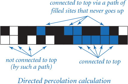
2.4.18 Fast percolation test. Modify the recursive _flow() function in PROGRAM 2.4.6 so that it returns as soon as it finds a site on the bottom row (and fills no more sites). Hint: Use an argument done that is True if the bottom has been hit, False otherwise. Give a rough estimate of the performance improvement factor for this change when running percplot.py. Use values of n for which the programs run at least a few seconds but not more than a few minutes. Note that the improvement is ineffective unless the first recursive call in _flow() is for the site below the current site.
2.4.19 Bond percolation. Compose a modular program for studying percolation under the assumption that the edges of the grid provide the connectivity. That is, an edge can be either empty or full, and a system percolates if there is a path consisting of full edges that goes from top to bottom. Note : This problem has been solved analytically, so your simulations should validate the hypothesis that the percolation threshold approaches 1/2 as n gets large.
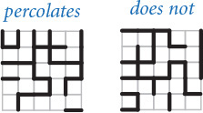
2.4.20 Bond percolation on a triangular grid. Compose a modular program for studying bond percolation on a triangular grid, where the system is composed of 2n2 equilateral triangles packed together in an n-by-n grid of rhombus shapes and, as in the previous exercise, the edges of the grid provide the connectivity. Each interior point has six bonds; each point on the edge has four; and each corner point has two.
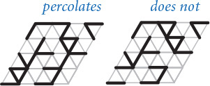
2.4.21 Percolation in three dimensions. Implement modules percolation3d.py and percolation3dio.py (for I/O and random generation) to study percolation in three-dimensional cubes, generalizing the two-dimensional case studied in this chapter. A percolation system is an n-by-n-by-n cube of sites that are unit cubes, with probability of being open p and probability of being blocked 1–p. Paths can connect an open cube with any open cube that shares a common face (one of six neighbors, except on the boundary). The system percolates if there exists a path connecting any open site on the bottom plane to any open site on the top plane. Use a recursive version of _flow() like the one in PROGRAM 2.4.6, but with eight recursive calls instead of four. Plot percolation probability versus site vacancy probability for as large a value of n as you can. Be sure to develop your solution incrementally, as emphasized throughout this section.
2.4.22 Game of life. Implement a module life.py that simulates Conway’s game of life. Consider a boolean matrix corresponding to a system of cells that we refer to as being either live or dead. The game consists of checking and perhaps updating the value of each cell, depending on the values of its neighbors (the adjacent cells in every direction, including diagonals). Live cells remain live and dead cells remain dead, with the following exceptions:
• A dead cell with exactly three live neighbors becomes live.
• A live cell with exactly one live neighbor becomes dead.
• A live cell with more than three live neighbors becomes dead.
Test your program with a glider, a famous pattern that moves down and to the right every four generations, as shown in the diagram below. Then try two gliders that collide. Then try a random boolean matrix, or use one of the starting patterns on the booksite. This game has been heavily studied, and relates to foundations of computer science (see the booksite for more information)
