8.2.1 Theory of static network reduction

A power system equivalent is a mathematical model intended to represent a large portion of a power system network that may contain generation plant, network branches, load or any combination of these. Figure 8.1 illustrates the general case of a large interconnected network divided into two parts or subsystems where one part is to be reduced to a small equivalent network whereas the second part is to be retained in full. The two parts are connected by a number of boundary circuits. The derivation of the power system equivalent is carried out by a network reduction process and Figure 8.1 shows the terminology used.

Figure 8.1 Illustration of static network reduction terminology used in the calculation of power system equivalents

Network reduction is effectively a mathematical process that combines and eliminates network nodes and branches, so that the reduced equivalent contains smaller number of nodes and branches than the original network. The equivalent must be capable of reproducing the electrical behaviour of the original network at the boundary interface or nodes with sufficient accuracy. There are several types of power system equivalents the characteristics of which depend on the type of power system analysis being carried out. Equivalents may generally be classed as static or dynamic equivalents. The former may be used in dc and ac loadflow analysis, ac short-circuit analysis and harmonic analysis etc. The latter are used in power system stability and control analysis. In this chapter, we are concerned with the derivation of power system equivalents by network reduction for use in power system short-circuit analysis.

To illustrate the theory, subsystem 1 in Figure 8.1 is the power system network whose reduced equivalent is to be calculated as seen from nodes 1 to N which are termed the boundary nodes. All internal nodes and branches in subsystem 1 are to be eliminated in deriving the equivalent seen ‘looking’ from the boundary nodes into subsystem 1. The equivalent, as seen from the boundary nodes 1 to N consists of these nodes only, self (shunt) impedances to the reference node, usually the zero voltage node, and transfer impedances between all boundary nodes. All internal nodes and their interconnecting elements, e.g. lines, cables, transformers, etc., within subsystem 1 are to be eliminated by the reduction process. The reduced equivalent is illustrated in Figure 8.2. Both the boundary circuits and subsystem 2 are excluded from the reduction process.

Figure 8.2 Illustration of the power system equivalent produced by the network reduction process of subsystem 1 of Figure 8.1

The number of boundary nodes should not be very large otherwise a very large number of transfer or series branches will be generated between all boundary nodes in the equivalent and this is equal to N(N − 1)/2, where N is the number of boundary nodes. For example, if the original full network of subsystem 1 consists of 500 nodes and 1000 series branches, a 50-boundary node equivalent of subsystem 1 will result in a 1225 series branches!

8.2.2 Need for power system equivalents

During the early days of power system network analysis by digital computers, the need for network equivalents arose in order to allow the analysis of large-scale power systems to be practically possible given the limited computer storage and speed at that time. However, due to the huge developments in computer technology, this constraint is no longer applicable and very large power systems can nowadays be analysed quickly and cost effectively on personal computers.

However, power system equivalents are still required in industry. Practical examples include a distribution network company that owns and operates a distribution network and obtains its bulk power needs from a transmission company from one or several substations. The transmission network may be very large and an equivalent at one or more boundary nodes that are judiciously selected is usually sufficient for the short-circuit analysis needs of the distribution company. Similarly, the transmission company itself would not need to represent the distribution network in its entirety and an appropriate equivalent at one or more boundary nodes is usually sufficient. The added practical advantages are that the exchange and processing of data between companies is simplified, extraneous networks are removed from studies and the volume of data to be exchanged is reduced thus minimising the scope for errors in data handling. In general and in order to maintain sufficient accuracy of calculated short-circuit currents, experience shows that the network voltage level being studied should be represented in full as well as individual transformers stepping up or down to the next voltage level. For example, consider a network consisting of the following voltage levels: 400 kV transmission; 132 kV subtransmission; 33, 11 and 0.43 kV distribution. If the voltage level being studied is 132 kV, then the 132 kV network should be modelled in its entirety (all lines, cables, series reactors, etc.) as well as all 132 kV/400 kV autotransformers, 132 kV/33 kV and 132 kV/11 kV transformers. Power system equivalents may be placed at 400, 33 or 11 kV voltage levels if required as this will generally have a negligible effect on the precision of the results of short-circuit currents calculated on the 132 kV network.

Further, the ongoing liberalisation, restructuring and privatisation of electricity supply industries around the world since the 1990s have created the need for the calculation of equivalents. Generally, new electricity trading markets and new market participants are established, e.g. independent generating companies (Gencos), independent transmission system owners and/or operators (TSOs) and independent distribution system owners and/or operators (DSOs). Figure 8.3 illustrates some typical exchange requirements of either detailed network data or power system equivalents among the main participants in a typical electricity market. The actual flow of data may differ from one market to another depending on whether network owners are also operators of networks owned by other companies.

Figure 8.3 Illustration of exchange requirements of detailed network data or power system equivalents in a liberalised electricity market

Normally, network codes are also established that include legal obligations for the exchange of planning and operational data between various companies and much of the detailed technical data is usually classed as confidential. As a result, using Figure 8.3, TSOs may be required to provide equivalents to DSOs and vice versa. TSOs may also exchange equivalents among themselves but where the accuracy of these equivalents is of critical importance in terms of operating safe and secure interconnected transmission networks, full network data may be exchanged. Gencos and large industrial consumers are usually required to provide full network data to their host network operators who may not be allowed to pass it on to other network users due to confidentiality.

8.2.3 Mathematical derivation of power system equivalents

Conventional bus impedance or admittance matrices

Various mathematical methods can be used to carry out the network reduction process and derive the required power system equivalent. Most methods use either the bus impedance matrix or the bus admittance matrix of the entire network. For a W node network, let the bus impedance matrix be given by

     (8.1)

For a given set of boundary nodes N, an impedance submatrix Z_Bound, whose diagonal terms correspond to the boundary nodes, can be extracted from the full network impedance matrix of Equation (8.1). For example, if the boundary nodes are nodes 2, 5 and 9, then Z_Bound is given by

     (8.2)

In the general case of N-boundary nodes, and renumbering the nodes 1 to N for convenience, Z_Bound is given by

     (8.3)

The terms of Z_Bound are directly extracted from the full network bus impedance matrix. Therefore, the diagonal terms represent the driving point or Thévenin’s impedances seen at the boundary nodes and the off-diagonal terms represent the transfer impedances between the boundary nodes. The nodal admittance matrix of the boundary nodes Y_Bound is obtained by inverting Z_Bound as follows:

     (8.4a)

where

     (8.4b)

The diagonal element of node i, Y_ii is the sum of all admittances connected to node i including the shunt admittance y_ii to the reference node. Therefore, the shunt admittance connected at boundary node i is calculated by summing all the elements of row i of Equation (8.4a). An off-diagonal element in the nodal admittance matrix of Equation (8.4a) is equal to the negative of the admittance connecting the boundary nodes i and j.

Using Equation (8.3), the calculation of a single-node equivalent results in a single equivalent impedance admittance, as shown in Figure 8.4, as follows:

Figure 8.4 Power system equivalent of a single-boundary node

     (8.5)

Similarly, the calculation of a two-node equivalent using Equation (8.3) results in the following nodal impedance and nodal admittance matrices:

     (8.6a)

and its inverse, using Equation (8.4) is expressed as

     (8.6b)

Equation (8.6) is general and allows for a situation where these matrices are non-symmetric, i.e. Z₁₂ ≠ Z₂₁ and y₁₂ ≠ y₁₂ such as in the case of quadrature boosters or phase shifting transformers as discussed in Chapter 4. For symmetric matrices, the two-node equivalent can be represented as a star equivalent impedance or a Π equivalent admittance circuit as shown in Figure 8.5.

Figure 8.5 Power system equivalent for two-boundary nodes: (a) star impedance equivalent and (b) π admittance equivalent

Again, assuming symmetric matrices, the calculation of a three-node equivalent results in the following matrices:

     (8.7a)

and

     (8.7b)

The three-node equivalent can be represented as a star equivalent impedance or Π equivalent admittance circuit as shown in Figure 8.6.

Figure 8.6 Power system equivalent for three-boundary nodes: (a) star impedance equivalent and (b) π admittance equivalent

It is interesting to note that two-boundary nodes are described by a single-Π equivalent circuit whereas for three-boundary nodes, three-Π equivalents are required. Therefore, it is to be expected that the calculation of a multiple-node equivalent results in multiple-Π equivalent networks. Although a one-node increase in the number of boundary nodes adds one shunt impedance only, it, however, adds transfer admittances/impedances to all the original boundary nodes. Therefore, the number of transfer admittances/impedances rises rapidly with the number of boundary nodes. In practice, the transfer admittance/impedance between any two nodes is equal to the apparent impedance between these nodes in the original unreduced network. Thus, some transfer impedances will be very large (admittances very close to zero) where nodes are electrically quite remote from each other and hence these branches may be neglected.

Direct derivation of admittance matrix of power system equivalents

The conventional method described above requires the derivation of the entire network bus impedance matrix using techniques such as formulating and indirectly inverting the bus admittance matrix or by a step-by-step impedance matrix building process. An alternative is to derive the admittance matrix of the reduced equivalent directly from the full network admittance matrix given a specified number of boundary nodes. Figure 8.7(a) shows an interconnected passive linear network with N-boundary nodes and it is required to reduce the entire network to an equivalent as seen from these boundary nodes. All passive elements, e.g. lines, cables and transformers, are represented by their appropriate impedances. Rotating machines, e.g. synchronous generators are represented by an appropriate positive phase sequence (PPS) impedance such as subtransient or transient impedance, and their voltage sources are short-circuited.

Figure 8.7 Direct derivation of a power system equivalent of N-boundary nodes: (a) network to be reduced as seen from N-boundary nodes and (b) multiple-π equivalent admittance circuit

In the calculation of negative phase sequence (NPS) and zero phase sequence (ZPS) equivalents, the machines are represented by their NPS and ZPS impedances to earth. The technique is based on the connection of a voltage source at each boundary node in turn, measuring the injected current into the boundary node and the resultant voltages at all other boundary nodes. The injected voltage source at each boundary node must have the same magnitude and phase angle, if any, though the latter may be zero. The magnitude of the voltage source is arbitrary, but a sufficiently large value may be used to improve the precision of calculated parameters.

The objective is to derive the equivalent nodal admittance matrix of the N-boundary nodes which is represented by the multiple-Π circuit of Figure 8.7(b). A current I₍₁₎ injected into node 1 will produce currents and voltages throughout the network including voltages at the boundary nodes 1, 2, 3,…, N. From Figure 8.7(b), we can write

     (8.8)

wherein y₁₁ is the shunt admittance between node 1 and the reference node, y₁₂ is the transfer admittance between nodes 1 and 2, V₁₍₁₎ is the voltage at node 1 due to injected current I₍₁₎, V_>2(1) is the voltage at node 2 due to injected current I₍₁₎, etc. Rearranging Equation (8.8), we obtain

     (8.9a)

where

     (8.9b)

At boundary node 2, where the injected current is 0, we can write

or

     (8.10a)

where

     (8.10b)

and similarly for nodes 3, 4, 5,…, N. For node N, we obtain

     (8.11a)

where

     (8.11b)

Equations (8.9a) and (8.10a) to (8.11a) can be written in matrix form as follows:

     (8.12)

The process is now repeated for boundary node 2. A current I₍₂₎ is now injected into node 2 and this will produce currents and voltages throughout the network including voltages at the boundary nodes 1,2, 3,…, N. Using a similar derivation process to that of Equation (8.12), we obtain

     (8.13)

Continuing with the above current injection process, i.e. to boundary nodes 3,4,…, N, writing the derived equations in matrix form in each case, we can collect the individual matrix Equations (8.12), (8.13), etc., into the following system of matrix equations:

     (8.14)

or in concise matrix form

     (8.15)

where I_{N × N} is a diagonal N × N matrix of known injected currents and V_{N × N} is a known N × N non-symmetric matrix of resultant voltages, i.e. V₁₍₂₎ ≠ V₂₍₁₎ in the general case. Knowing the injected currents and voltages into the boundary nodes, the equivalent admittance matrix of the TV-boundary nodes can be calculated as follows:

     (8.16)

where Y_{N × N} is a general non-symmetric admittance matrix. In most practical system networks, Y_{N × N} is actually a symmetric matrix. The admittance connecting node i to any other boundary node, e.g. y_ij, is equal to the negative of the corresponding off-diagonal element of Y_{N × N}. The shunt admittance at boundary node i shown in Figure 8.7(b) is given by

     (8.17)

The impedances of the admittance branches of Figure 8.7(b) are calculated as follows:

     (8.18a)

and

     (8.18b)

In practical applications, the technique described above can be used to calculate more than one PPS equivalent such as subtransient and transient equivalents corresponding to subtransient and transient reactances of machines. In deriving the PPS equivalent, and depending on the national approach followed, line and cable shunt susceptance and shunt admittance of static loads may be excluded. In addition, the technique can also be directly applied to the calculation of NPS and ZPS equivalents. The shunt elements that may be excluded in the PPS equivalent calculation may also be excluded in the NPS equivalent calculation but they are generally included in the calculation of the ZPS equivalent.

Generalised time-dependent power system equivalents

Power system PPS, NPS and ZPS equivalents are calculated and included in PPS, NPS and ZPS models of the power system network used to calculate both balanced and unbalanced short-circuit fault currents. A generalised PPS time-dependent power system equivalent for a single node consists of a voltage source behind a series PPS impedance. The source voltage is the PPS Thévenin’s or open-circuit voltage and the PPS impedance consists of a resistance in series with a time-dependent reactance. In the general case where the equivalent contains active sources, a generator model can be used to represent the equivalent whose PPS reactance at any point in time is given by

     (8.19)

where X_Eq, and are the steady state, transient and subtransient PPS reactances of the equivalent at the boundary node. and are the transient and subtransient time constants of the equivalent at the boundary node. The NPS and ZPS equivalent impedances at the boundary node, denoted 1, are and , respectively. Figure 8.8 illustrates the PPS, NPS and ZPS equivalents of a single-boundary node.

Figure 8.8 Sequence power system equivalents for a single-boundary node: (a) PPS time-dependent equivalent, (b) PPS subtransient equivalent, (c) PPS transient equivalent, (d) NPS equivalent and (e) ZPS equivalent

The sequence representation of a single-node equivalent can be extended to equivalents of two or more boundary nodes. The shunt branch connected at each boundary node in the π or multiple-π equivalents represents an equivalent source of short-circuit current, i.e. rotating plant. Figure 8.9 illustrates the PPS, NPS and ZPS π admittance circuit equivalents for two-boundary nodes.

Figure 8.9 Sequence power system equivalents for two-boundary nodes: (a) PPS subtransient π equivalent, (b) PPS transient π equivalent, (c) NPS π equivalent and (d) ZPS π equivalent

8.3.1 Representation of power generating stations

In a practical power system, the amount of installed generation plant exceeds the system peak demand by an appropriate margin, typically 20%, to allow for generation unavailability and demand forecasting errors. In order to maximise the magnitude of calculated short-circuit currents in planning and design studies, all generation plant is usually assumed operating but appropriately scaled to match system demand plus power losses. For off-peak demand year round operational planning studies, usually only scheduled generation dispatched to meet system demand, system frequency control and operating reserves may be used in the calculation of short-circuit currents.

In Chapter 5, we discussed the modelling of individual generators for short-circuit analysis purposes. In a power station comprising a number of generators that may be connected to the power system network being studied either directly or through their own step-up transformers, the precision in the calculated short-circuit currents is generally improved if each generator is represented individually. However, the representation of power stations as equivalents is generally adequate if they are electrically quite remote from the locations being studied.

As presented in Chapter 5, power stations driven by renewable energy sources such as wind are being connected in increasing numbers and sizes both to distribution and transmission networks. A single wind farm power station may comprise, tens to hundreds of generators rated at, say, 2 to 5 MW each. The large number of small generators in such a wind farm may be comparable to the total number of large generators individually modelled in the entire network of an average size utility. Figure 8.10(a) illustrates a typical layout of a 128 MW offshore wind farm consisting of eight rows of eight wind turbines each and each wind turbine generator is rated at 2 MW. Each turbine generator has its own transformer that steps up to medium voltage, typically 20–33 kV, and all are connected by cables to a single collector busbar.

Figure 8.10 Offshore wind farm and sequence equivalents: (a) typical layout of a 128 MW wind farm (64 generators) and (b) sequence equivalents at collector busbar (boundary node(s))

The wind farm may be modelled in its entirety including all 64 generators for local wind farm connection design studies. However, for studies at electrically remote locations on the wider host distribution, subtransmission or transmission systems, a reduced short-circuit equivalent for the wind farm generators, their transformers and cables at the collector busbar is usually sufficient. PPS, NPS and ZPS equivalents would be required to completely describe the equivalent as illustrated in Figure 8.10(b). The ZPS equivalent impedance is usually infinite because the transformer is usually delta-star connected.

8.3.2 Representation of transmission, distribution and industrial networks

For short-circuit analysis on transmission systems, transmission networks are usually modelled in their entirety in order to avoid loss of accuracy of calculated short-circuit currents. Generators connected to transmission networks are modelled in full and distribution networks supplied from a transmission network are modelled in part with appropriate equivalents for the remainder.

For short-circuit analysis on distribution systems, distribution networks may be modelled in their entirety as well as generators connected to these networks. Transmission networks supplying these distribution networks may be modelled using appropriate equivalents.

For short-circuit analysis in power station auxiliary systems or industrial power systems where a significant number of motors of different sizes may be used, a full representation of the entire station auxiliary and industrial networks is usually required. However, groups of parallel low voltage, e.g. 0.415 kV may be lumped together to form a single equivalent model for each. The modelling of motors above 1 kV individually improves calculation accuracy.

Where ac superposition analysis is used, general power system static load at bulk supply substations in transmission and distribution networks is usually modelled as shunt PPS and NPS impedances derived from the prefault load voltage, MW and MVAr demand. The load ZPS impedance is derived from the network and transformer impedances that provide a path for ZPS currents. Where required by national practice, small induction motors forming part of the general substation load may be modelled as an equivalent motor connected at the substation.

8.4.1 Superposition analysis and initial ac loadflow operating conditions

The magnitude of short-circuit current is primarily determined by the amount of connected generation plant and network topology. Where the superposition analysis technique is used, such as that described by the UK ER G7/4 guide, and although of secondary influence, the effect of initial network and generating plant operating conditions is nonetheless important when assessing the short-circuit duties on existing switchgear. A loadflow operating condition that gives a particular network voltage profile, transformer tap positions and machine internal voltages that maximise the short-circuit current at one location, will not necessarily do so at other locations in the network. For example, short-circuit currents at locations remote from generation plant will be higher for higher prefault voltages at these locations. However, at generating stations with generator-transformers equipped with on-load tap-changers, the short-circuit currents delivered on the high voltage side of the transformers will be higher for lower prefault voltage on the transformer high voltage side. This is because the fault currents delivered from this power station unit depend on the ratio of the generator impedance to transformer impedance and on the transformer tap position. Similarly, a lower voltage profile on a subtransmission or distribution system, e.g. 132 kV, will generally cause an increase in the short-circuit current delivered through autotransformers from the transmission system, e.g. 275 or 400 kV. Also, a lower voltage at 132 kV together with a higher voltage at 33 or 11 kV will cause higher short-circuit currents at 33 and 11 kV delivered through the 132 kV/33 kV and 132 kV/11 kV transformers which are equipped with high voltage winding on-load tap-changers. Therefore, in calculating maximum short-circuit currents at various locations in a power system, there may be conflicting requirements in the loadflow study, so that a single study cannot be established to calculate maximum short-circuit currents at various locations.

8.4.2 Effect of mutual coupling between overhead line circuits

In Chapter 3, we showed that for double-circuit overhead lines, there will be like sequence PPS, NPS and ZPS couplings between the two circuits where six-phase transpositions are assumed and ZPS coupling only where ideal nine-phase transpositions are assumed. The PPS/NPS inter-circuit mutual impedances are generally small and typically only a few per cent of the PPS/NPS self-circuit impedances. However, the ZPS inter-circuit mutual impedance can be significant in comparison with the ZPS self-circuit impedance. To illustrate the effect of ZPS mutual coupling on the magnitude of the ZPS short-circuit current, consider the ZPS representation of a double-circuit overhead line shown in Figure 8.11(a) where the two circuits are denoted A and B.

Figure 8.11 Effect of ZPS mutual coupling between two overhead line circuits: (a) ZPS inter-circuit coupling with both circuits in service; (b) ZPS inter-circuit coupling with one circuit out of service and earthed at both ends

Using Equation (3.89a) from Chapter 3, the series voltage drop across circuits A and B are and The effective ZPS impedance of each circuit is given by and if the ZPS currents and are equal and flow in the same direction. However, if the ZPS currents are equal but flow in the opposite direction, and . Therefore, if the ZPS mutual impedance between the two circuits is neglected in the modelling of the line, the short-circuit current calculated may be either an overestimate or an underestimate depending on the direction of ZPS currents flowing in each circuit. Where the ZPS currents flow in the same direction, there will be an overestimate but where the ZPS currents in each circuit flow in opposite directions, there will be an underestimate.

Figure 8.11(b) shows another practical case of a double-circuit overhead line with two identical circuits and with one circuit assumed of service and earthed at both ends for safety reasons. The voltage drops across each circuit are given by and . Since circuit B is earthed at both ends,

Therefore, the effective impedance of the in-service circuit A is given by

For example, for a typical 400 kV double-circuit line used in England and Wales with four subconductor bundle per phase, the ZPS impedance per circuit and the ZPS mutual impedance between the two circuits are = (0.103 + j0.788)Ω/km and = (0.085 + j0.420)Ω/km, respectively. Therefore, the effective impedance of one circuit with the second circuit earthed at both ends is equal to = (0.0415 + j0.565)Ω/km. This represents a 28.7% reduction in the magnitude of the series impedance and an increase in its effective X/R ratio from 7.6 to 13.7. The increase in X/R ratio occurs because the phase conductors of the earthed circuit effectively act as short-circuited secondary turns where a significant proportion of the return short-circuit current flows via these ‘turns’ and much less returns via the single conductor earth wire.

8.4.3 Severity of fault types and substation configuration

Figure 8.12 shows typical air and gas insulated substations that include several circuit-breakers. For the assessment of the making and breaking (interrupting) duties of existing circuit-breakers, the selection of new circuit-breakers or the assessment of substation infrastructure integrity, both three-phase and single-phase short-circuit fault currents are usually calculated. In isolated or high impedance earthed systems, three-phase fault calculations are sufficient but for solidly earthed systems such as 132 kV and above in the UK, single-phase fault currents have to be calculated as well. Single-phase short-circuit currents will be higher than three-phase short-circuit currents at locations where the ZPS equivalent impedance at the fault point is lower than the PPS/NPS impedance. Figure 8.13(a) shows the direction of short-circuit currents for a close-up fault at F before fault clearance in a double-busbar or transfer bus substation layout. The maximum short-circuit breaking (interrupting) duty on circuit-breaker A is calculated assuming it is the last circuit-breaker to open to clear the fault, i.e. all circuit-breakers B, C and D have already opened. This duty can also occur under automatic circuit-breaker reclosure onto a persistent short-circuit fault. The two duty conditions are depicted in Figure 8.13(b).

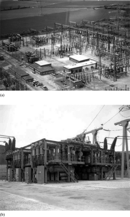
Figure 8.12 Air and gas insulated substations: (a) 400 kV outdoor air insulated substation and (b) 275 kV outdoor gas insulated substation

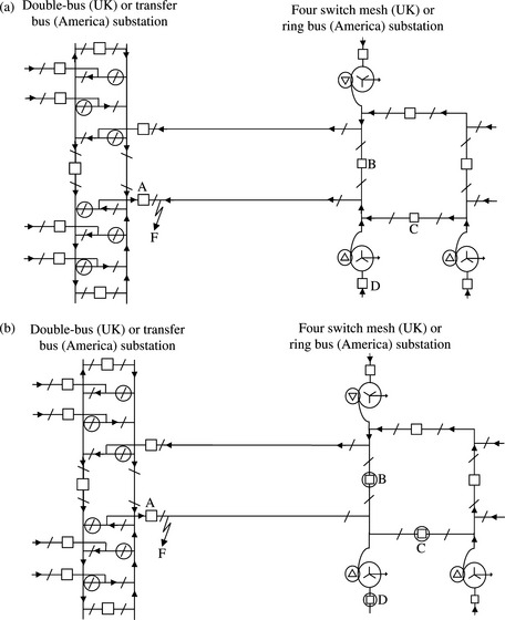
Figure 8.13 Illustration of the effect of substation configuration on maximum short-circuit currents: (a) direction of current flows for a short-circuit fault at F before fault clearance and (b) A is last circuit-breaker to clear short-circuit fault F or A recloses onto a persistent fault F by automatic circuit reclosure

Bus coupler and bus section circuit-breakers, shown as A and B in Figure 14.8(a) and (b) are required to make and interrupt the maximum fault current associated with short-circuit infeeds from all connected circuits when energising a section of busbar which is still inadvertently earthed. The resultant direction of current flow in the substation is also indicated. The making onto such a fault also imposes maximum duty on substation infrastructure equipment.

Figure 8.15(a) illustrates the direction of short-circuit current flows for a close-up fault on an outgoing line in a 1 and ½ circuit-breaker substation where circuit-breaker A or B being the last to open will be required to clear the fault. Figure 8.15(b) illustrates a busbar short-circuit fault on the same substation configuration, cleared by opening of circuit-breakers A, B, C and D with the last to open seeing the duty.

Figure 8.15 Short-circuit currents in ‘1 and 1/2’ circuit-breaker substations: (a) direction of current flows for a close-up short-circuit fault on a line at F before fault clearance and (b) direction of current flows for a short-circuit busbar fault at F before fault clearance

8.6.1 Background

The international standards of short-circuit current calculation, IEC 60909 and IEEE C37.010 are essentially deterministic in approach. The former is aimed at calculating results with acceptable accuracy for their intended purpose and the latter is generally aimed at calculating sufficiently conservative results. The UK ER G7/4 approach is also deterministic although it is aimed at the calculation of worst-case realistic results. These approaches include various assumptions aimed at calculating maximum values of short-circuit currents. On the other hand, probabilistic short-circuit analysis techniques are generally aimed at calculating a probability distribution of short-circuit current magnitudes at various locations in the system. This can provide information on the probability of short-circuit currents exceeding certain values or falling below certain values.

8.6.2 Probabilistic analysis of ac short-circuit current component

Probabilistic analysis techniques of ac short-circuit current component recognise that the magnitude of short-circuit current at a given location is primarily determined by the following three random statistical factors:

The deterministic short-circuit analysis approach considers (a) and (b) above although not faults some distance away from substations except where tower currents are being calculated. However, for network design studies, this approach does not consider (c) but instead it usually assumes that all installed generation plant is available and connected to the network and can contribute short-circuit current. The network elements e.g. lines and transformers etc are all assumed to be 100% available. In network operational planning studies, 100% availability of generation plant and network may be assumed in the area close to the faulted locations but not on a system wide basis.

The probabilistic short-circuit analysis approach aims at avoiding the compounding of safety factors or the assumption of simultaneous coincident worst case conditions. Thus, many power system states are considered and analysed at the time of occurrence of the fault and a fault current is calculated for each state.

The probability distributions of the calculated short-circuit current magnitudes may be compared to the deterministic or probabilistic rating of circuit-breakers or busbars, as required, as illustrated in Figure 8.16(a) in a typical 400 kV system.

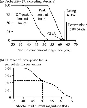
Figure 8.16 Illustration of probabilistic analysis results of short-circuit current ac component in a 400 kV transmission system: (a) probability distribution of ac short-circuit current magnitude and (b) risk of three-phase short-circuit faults exceeding abscissa

The current magnitude calculated by the deterministic approach is 64 kA and is greater than the circuit-breaker rating of 63 kA. The maximum current calculated by the probabilistic approach for peak demand hours is 65 kA. Assuming a 1 kA safety margin is used, there is a 2% probability of exceeding 62 kA. These results may be combined with an assumed uniform probability of three-phase fault occurrence throughout the year per substation, in the absence of better information. The outcome is illustrated in Figure 8.16(b). This shows that 0.023 faults per annum exceed 50 kA or a risk of one fault in 43.5 years exceeding 50 kA. Also, this shows that 0.04 faults per annum exceed 62 kA or a risk of one fault in 250 years exceeding 62 kA. The off-peak demand hours show much lower short-circuit currents due primarily to the reduced amount of connected generation plant.

Monte Carlo simulations may be used to simulate the behaviour of the power system under fault conditions by applying faults at random times during a year of system operation and at random locations in the network. However, the description of such simulations is outside the scope of this book. Probability distributions of subtransient, transient or other intermediate short-circuit current magnitudes may be calculated.

8.6.3 Probabilistic analysis of dc short-circuit current component

Factors affecting dc short-circuit current magnitude

In IEC 60909 and as implied in IEEE C37.010 and ER G7/4, evolving short circuit faults are not considered. Therefore, a three-phase short circuit is assumed to occur simultaneously on all three phases. This is important because sequential short-circuit faults can lead to dc current asymmetry greater than 100% but this is not dealt with in this book.

Recalling Equation (1.17) derived in Chapter 1 for the dc short-circuit current component following a simultaneous three-phase short-circuit fault, we have

     (8.20)

where

     (8.21)

and

     (8.22)

The magnitude of the dc current component in any phase depends on the magnitude of the initial or subtransient ac current component I_rms and the instant on the voltage waveform ϕ_r when the short circuit occurs. The rate of decay of the dc current component depends on the time constant L/R or initial X/R ratio at the fault point (X/R = ωL/R). The X/R ratio will vary with the fault location and fault type as well as the state of the system at the time of short circuit. The system state is determined by the availability of generation plant and network elements as well as the availability of any induction motor short-circuit infeed. The probability distributions of initial three-phase and single -phase X/R ratios at a 400 kV location comprising a large power station, a number of transmission circuits and a local distribution load are illustrated in Figure 8.17. The X/R ratios are calculated using IEC 60909 Method C. The results shows that the rated X/R ratios are almost always exceeded at such a location.

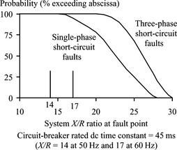
Figure 8.17 Illustration of a typical probability distribution of X/R ratio of de short-circuit current

From Equation (8.20), the initial magnitude of the dc current component in any phase at the instant of short circuit, t = 0, expressed in per cent of the peak ac short-circuit current component is given by

     (8.23)

Maximum dc current offset or full asymmetry assumed by the deterministic IEC, IEEE and ER G7/4 calculations occurs for ϕ - tan⁻¹(ωL/R) = - π;/2 or

     (8.24)

At any value of phase R angle ϕ_r, one or two dc current components will be negative. However, since we assumed a simultaneous three-phase fault condition, it is instructive to plot the absolute value of Equation (8.23) and this is shown in Figure 8.18. The initial dc current is plotted against the voltage phase angle ϕ_r for the IEC 62271 and IEEE C37.04 circuit dc time constant of 45 ms as well as the additional maximum quoted IEC 62271 circuit dc time constant of 120 ms. It is shown that for any value of ϕ_r, one of the three phases will have a dc current component of at least 86.6%. The effect of the dc time constant on the initial magnitude of the dc current is, as expected, negligible.

Figure 8.18 Absolute initial magnitude of dc current component in the three phases under a simultaneous three phase short-circuit fault

The above analysis assumed a simultaneous three-phase short-circuit fault. In the case of a circuit-breaker being inadvertently closed onto a network where a three-phase short-circuit fault already exists, as discussed in Section 8.4.3, the above analysis will equally apply if it is assumed that the three poles of the circuit-breaker close simultaneously. In practice, the three poles do not close mechanically at the same time due to pole stagger or span which, according to IEC 62271 Standard, should not exceed half cycle of power frequency (10 ms for 50 Hz systems and 8.33 ms for 60 Hz systems). Also, electrical closure or prestrike may occur before mechanical closure and this is discussed in the next section.

Probabilistic analysis of voltage phase angle ϕ

In practice, the deterministic assumption of maximum dc offset has a substantial impact on the sizing of circuit-breakers and substation infrastructure such as busbars particularly with the increasing X/R ratios in power systems. The assumption of near to zero voltage phase angle ϕ_r results in maximum dc offset so the question is: For non-simultaneous closure of the three circuit-breaker poles when closing onto a fault, what is the probability of one of the poles closing at a voltage phase angle near zero?

Now, we describe the factors that can give rise to the dispersion between the three circuit-breaker poles. First, we note that there are two distinct cases relating to whether the circuit-breaker is independent pole operated, i.e. has one closing mechanism per pole, or three-pole operated, i.e. has one closing mechanism driving all three poles. The latter results in near simultaneous mechanical closure so that the mechanical dispersion is very small, controllable and fixed. However, for circuit-breakers with independent pole operation, larger and variable dispersion can occur since there is no mechanical coupling between the three poles. Further, for any pole, using Figure 8.19, there is a dispersion in the time lag between the closing order T_co and the instant of actuation of the closing mechanism T_a. Second, there is a dispersion in the operating time between actuation and instant of mechanical closure when contacts touch T_mc. Also, electrical closures due to electrical breakdown or prestrikes between the approaching contacts, at T_ec, may occur. These parameters are illustrated in Figure 8.19 for a single phase or pole of the circuit-breaker. Curve (i) is a cosinusoid of period 4 × T_mc and indicates the time variation of pole 1 gap withstand voltage during closing, assuming the dielectric strength of the insulation medium to be constant. Curve (ii) indicates the system voltage across pole 1 gap of the circuit-breaker. As the withstand voltage of pole 1 contact gap falls to the level of voltage across the gap, an electrical closure or prestrike occurs at T_ec before the contacts mechanically touch. Similar process may occur for poles 2 and 3 of the circuit-breaker. The latter part of curve (i) can be approximated as a straight line and indicated by curve (iii) whose negative slope is defined as S where S = dv/dt = average rate of decay of dielectric strength of the gap during circuit-breaker closing in kV/s = (dielectric strength of the insulation medium in kV/cm) × (relative speed of approach of the contacts at impact in cm/s).

Figure 8.19 Illustration of circuit-breaker electrical closure, or prestrike, and mechanical closure

To derive an expression for the probability density function of the voltage phase angle ϕ, we neglect the voltage polarity effect on the electrical strength of the gap, i.e.. Figure 8.20(a) illustrates the mechanical closing instants and the corresponding range of electrical closing instants or angles for two different slopes S₁ and S₂ and Figure 8.20(b) shows an expanded section of a small element on the voltage curve.

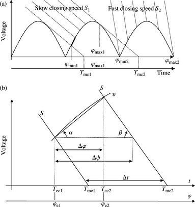
Figure 8.20 Probabilistic analysis of voltage phase angle of circuit-breaker closure onto a fault: (a) range of electrical closing angle due to a circuit-breaker prestrike and (b) an expanded section of a small element on the voltage curve of Figure 8.20(a)

Using Figure 8.20(b), consider two closing curves of the same slope S separated by a small time interval Δt, T_mc1 and T_mc2 are their respective mechanical closing times and T_ec1 and T_ec2 are their respective electrical closing instants. On the voltage waveform, the electrical phase angles ϕ_e1 and ϕ_e2 correspond to the time instants T_ec1 and T_ec2, respectively. The probability element of electrical closing between ϕ_e1 and ϕ_e2 is F(ϕ)δϕ where F(ϕ)δϕ is the probability density function of angle ϕ. The probability element between the mechanical closure instants T_mc1 and T_mc2 is F(t)δt where F(t) is the probability density function of mechanical closure with time t. Therefore, with ϕ and t being two functionally connected stochastic variables, we can write

     (8.25)

or

     (8.26)

The instant when the circuit-breaker closing order is given is random and is independent of the voltage phase angle ϕ and the breaker closes independently of time. Thus, the mechanical closing instant is uniformly distributed and has a constant probability density F(t) between the minimum and the maximum closing angles of 0 and Π as shown in Figure 8.20(a). Thus,

     (8.27)

However, the instant at which electrical closure, or prestrike, occurs is correlated with the voltage across the circuit-breaker contact gap. Thus, the distribution of the electrical closing instant, or angle, will not be uniform. From the geometry of Figure 8.21(b), we have

Figure 8.21 Probability density and distribution of electrical closing angle of a 400 kV circuit-breaker: (a) probability density of electrical closing angles and (b) probability of electrical closing angles

     (8.28)

where S is the slope of the closing curve and is negative, tan α is the slope of the source voltage i.e. .

From these relations and Equation (8.28), we obtain

     (8.29)

Therefore, using Equations (8.27) and (8.29) in Equation (8.26), we obtain

     (8.30)

The probability distribution f(ϕ) of the closing angle being equal to or greater than ϕ is equal to

and is given by

     (8.31)

Besides probabilistic design and operational planning studies, the calculated probability equations may also be used in quantified risk assessments where calculated short-circuit currents may potentially exceed the rating of circuit-breakers. This is discussed in the next section.

For other causes of short-circuit currents, e.g. a lightning strike on top of a tower, then three scenarios may be considered. The first is where the magnitude of the lightning current is so large that the induced tower top voltage will cause back-flashover to the three phases of the circuit irrespective of the actual instantaneous value of the voltage on each phase. This is similar to the simultaneous three-phase short circuit where one of the phases will have an initial dc current component of at least 86.6%. The second scenario is where a substantial lightning strike directly hits one of the phases of the circuit and causes a short circuit. In this case, since the short circuit is effectively independent of the voltage magnitude or phase angle, the probability of the short circuit occurring between voltage zero and voltage peak is uniform. The probability of maximum dc current offset requires a short circuit at or near to voltage zero and if this is assumed to be within 0 ± 10°, then this equates to 40° over a full power frequency cycle of 360°. Therefore, the probability of maximum dc current offset is approximately equal to (40° /360°) × 100 ≈ 11%. The third scenario is where the magnitude of the lightning induced voltage alone is insufficient but together with that of the actual instantaneous value of the voltage on any one phase will cause back-flashover and short circuit. Under this mechanism, the short circuit is more likely to occur when the phase voltage is significantly away from voltage zero. In this case, the probability of maximum dc current offset arising may be assumed to be negligible.

It is noted that the variable S used in Equations (8.30) and (8.31) is an important circuit-breaker parameter for the practical application of point-on-wave closing technique of circuit-breakers. This application is aimed at reducing transient over-voltages such as when energising shunt capacitor banks. To achieve this, the technique aims at closing the three poles at or very close to voltage zero on the source voltage waveform which requires a high value of S. Therefore, a circuit-breaker equipped with point-on-wave closing will produce maximum dc offset in each phase if it were inadvertently closed onto an existing three-phase to earth short-circuit fault. The effect of the parameter S on the probability of closing at various voltage phase angles is illustrated in an example in the next section.

8.6.4 Example

8.7.1 Background

Short-circuit studies carried out in long-term network design short-term network operational timescales or real time may identify short-circuit duties on existing switchgear in excess of ratings. The condition is usually defined as switchgear that is potentially overstressed. In the unlikely event of switchgear being identified to be potentially permanently overstressed, and in the absence of operational solutions (this is discussed in the next chapter) to remove the condition, it is usual to replace such switchgear with higher rated equipment. In network operational planning timescales, temporary overstressing may be identified such as may occur during switching operations to reconfigure the network. Depending on operating practices, substation configurations and circuit definitions, the duration of such a potential temporary overstressing may extend from a few minutes to possibly an hour.

8.7.2 Relevant UK legislation

When the health and safety of employees and the general public is affected, there may be legal duties which must be observed. With reference to the UK, the relevant legislation can be summarised as follows:

Breaches of legislation in the UK are criminal offences and can lead to prosecution. Switchgear should not be overstressed if this gives rise to danger but if an employer takes all reasonably practicable steps and exercises all due diligence to avoid danger, a defence can be formed by the implementation of a suitable risk management procedure such as a quantified risk assessment.

8.7.3 Theory of quantified risk assessment

The objectives of quantified risk assessment are to identify the risk of fatality to an individual associated with equipment catastrophic failure and to reduce these individual risks to a level which is As Low As Reasonably Practicable (ALARP). The UK Health and Safety at Work Act 1974 includes the ALARP concept and the Health and Safety Executive have interpreted this concept in a risk diagram as shown in Figure 8.22.

Figure 8.22 The ‘ALARP’ principle of the UK’s Health and Safety at Work Act

The diagram consists of three regions. The ‘bottom broadly acceptable region’ is where the individual risk is so small that no further measures are necessary. The top ‘unacceptable region’ is where the individual risk is so large that it cannot be tolerated. The middle ‘ALARP region’ is where the individual risk must be ‘As Low As Reasonably Practicable’ considering the benefits of accepting the risk against the costs incurred of any further risk reduction measures. The UK Health and Safety Executive suggests certain numerical levels of risks. A risk of 10⁻⁷ or 1 in 10 million per person per year represents negligible risk. A risk level at the lower limit of the ALARP region is 10⁻⁶ or 1 in 1 million per person per year. Also, the suggested level of risk at the upper limit of the ALARP region is 10⁻⁴ or 1 in 10 000 per person per year for the public and 10⁻³ or 1 in 1000 per person per year for employees, respectively. The maximum tolerable level of risk to the public, 1 in 10 000 per person per year, is based on the proportion of people killed in road-traffic-related accidents in the UK per year. At the bottom of the ALARP region, the risk may be tolerated if the cost of reducing it would exceed the improvement gained. However, at the top of the ALARP region, the risk must be reduced unless the cost of reduction, which would exceed the improvement gained, is grossly disproportionate to the improvement gained.

8.7.4 Methodology of quantified risk assessment

A quantified risk assessment method consists of two steps: (a) risk analysis and (b) risk evaluation. Risk analysis may use an event tree risk analysis model in order to quantify the risks. This is a method originally devised to assess protective systems reliability and safety in nuclear power plants. Risk analysis consists of the following steps:

The individual risk (IR) is estimated as follows:

     (8.32)

Risk evaluation consists of comparing the estimated IR against the criteria for risk unacceptability, acceptability and tolerability as described in Section 8.7.3 and shown in Figure 8.22.