
10 An introduction to the analysis of short-circuit earth return current, rise of earth potential and electrical interference
10.1 Background
We outlined in Chapter 1, one area where short-circuit current calculations are made to calculate rise of earth potential at substations and at overhead transmission line towers. During an unbalanced single-phase to earth or two-phase to earth short-circuit fault, either the total earth fault current or a proportion of it will flow through the general mass of the earth and return to the source. The earth current will return to the neutral point(s) of the supply transformers or sources supplying the fault current through a substation earth electrode system that has a finite impedance. The product of the earth return current and the substation earthing impedance causes a rise in the potential of the substation earthing system and of the earth in the vicinity of the substation with respect to the potential of the general mass of the earth. Excessive rise of earth potential may be dangerous to people in the vicinity or may even cause damage to plant.
The flow of current in earth through a substation earthing system will produce potential gradients or contours within and around the substation. However, the detailed analysis of these contours using electromagnetic field theory is outside the scope of this book. Here, we present the calculation of rise of earth potential only at the location where the current enters earth.
The calculation of rise of earth potential requires the calculation of the earth return current or the proportion of earth fault current that returns through earth. We will present methods for the calculation of such currents that are generally accurate and sufficient in the majority of practical applications except where several long cable circuits emanate from the substation. In these cases, detailed multiphase modelling of connected equipment is recommended.
At substations, an earthing conductor is used to connect to earth exposed metal surfaces of various substation equipment. Because of its huge volume, the overall body of the earth is used as a reference, i.e. it has zero voltage. Earthing conductors do not normally carry current and should have a zero voltage, i.e. their voltage is identical to that of remote earth except under short-circuit conditions. An earth electrode is a part of the earthing system that is in contact with the earth and may comprise copper conductor, cast iron plates or steel piles, etc. Earthing of neutral points in a power system is made by the connection to the earthing electrode system of: substation equipment, metalwork, cladding, overhead line earth wires, cable sheaths and armouring terminating at the substation. In North America, the term grounding is used and is analogous to earthing.
10.2 Electric shock and tolerance of the human body to ac currents
10.2.1 Step, touch, mesh and transferred potentials
Electric shock may occur when a person touches an earthed structure during a short-circuit fault or walks within the vicinity of an earthing system during a fault or touches two separately earthed structures. Figure 10.1 illustrates a person in the vicinity of an ac substation subject to step, touch, mesh and transferred potentials. Step potential is the surface potential difference between the 2 ft of a person that are assumed to be 1 m apart. Touch potential is the potential difference between the hands and feet of a person when they are standing 1 m away from an earthed object they are touching with their hands. Mesh potential is the maximum touch potential to be found within a mesh of the substation earthing system. Transferred potential is a case of a touch potential in a remote location where the shock voltage may be approaching the full rise of earth potential of an earth electrode.

10.2.2 Electrical resistance of the human body
The human body presents a resistance (impedance) to the flow of ac power frequency current which decreases non-linearly with the applied touch voltage. Various parts of the human body such as skin, blood, muscles, tissues and joints, tend to oppose current flow. Broadly speaking, the human body presents an impedance that consists of two parts. The internal impedance which is mainly resistive, and the impedance of the skin at the point of contact which consists of a resistance and capacitance in parallel. Above about 200 V touch voltage, the dc resistance and ac impedance of the human body are generally equal.
Figure 10.2 shows a simplified representation of the resistances of the human body where the following equations can be written

Measurements of the hand-to-hand and hand-to-foot body resistances suggest that the arm and leg resistances are related by RLeg ≈ 0.6 × RArm. Thus,
and if both hands and both feet are in parallel
The above equations indicate that the effective resistance of interest is between extremities, e.g. from one hand to the other, from one hand to both feet or from one foot to the other. The resistance of internal body tissues is around 300 Ω excluding skin resistance. Including skin, the total resistance from hand to hand is typically between 600 and 3300 Ω. The total body resistance reduces with increasing touch voltage because of the considerable reduction in the skin resistance part due to damage or puncture. For example, for RHand-Hand = 1725 Ω at a 100 V touch voltage, RArm = 862.5 Ω, RLeg = 517.5 Ω, RHand-Foot = 1380 Ω, ROne hand-Both feet = 1121 Ω, RBoth hands-Both feet = 690 Ω, RBoth hands-Body centre = 431 Ω and RFoot-Foot = 1035 Ω. The most dangerous currents in terms of ventricular fibrillation of the heart (this is discussed in the next section) are those that flow from left hand to one or both feet. For other paths through the body, IEC 60479-1:2005 provide a rough estimation of the current magnitude required to present an equivalent danger of ventricular fibrillation. For example, for a left foot to a right foot path, the magnitude of the current required is 25 times higher. According to American IEEE Standard 80:2000, the total body resistance from one hand to both feet, hand to hand and foot to foot is generally taken equal to 1000 Ω.
10.2.3 Effects of ac current on the human body
The effects of an ac electric current passing through the vital parts of a human body depend on magnitude, frequency and duration of this current. The most common physiological effects of electric current on the human body, in order of increasing current magnitude, are perception, muscular contraction, unconsciousness, ventricular fibrillation, respiratory nerve blockage and burning. Accordingly, a number of touch current thresholds are defined such as perception, reaction or muscular contraction, let-go and ventricular fibrillation. The threshold of reaction is usually taken as 0.5 mA independent of duration. The threshold of let-go current is the maximum touch current at which a person can let-go of the electrodes they are holding. This threshold is assumed in IEC 60479-1:2005 to be equal to 10 mA for adult males and 5 mA for all population of adult males, females and children. Ventricular fibrillation is a condition of incoordinate action of the main chambers (ventricles) of the heart resulting in immediate arrest of blood circulation. Humans are vulnerable to the effects of power frequency currents and values as low as tens of mA can be lethal. In comparison with power frequency current, it is generally accepted that the human body can tolerate a slightly higher current at 25 Hz and approximately five times larger current at zero frequency i.e. dc current. Fortunately, the human body may tolerate hundreds of amperes in the case of lightning surges because of their very short microseconds duration. The threshold of perception is generally taken as 1 mA. Currents from 0.5 to 5 mA, usually termed let-go currents, do not impair the ability of a person holding an energised object to control his muscles and release it. From 5 mA with a duration of 7 s up to 200 mA with a duration at 10 ms, currents are quite painful. They can result in strong involuntary muscular contraction, difficulty in breathing and immobilisation but do not usually cause organic damage and the effects are temporary and would disappear if the current is interrupted. It is generally not until a current magnitude of around 100 mA that ventricular fibrillation, stoppage of the heart or inhibition of respiration might occur and cause injury or death. In such cases, resuscitation does not work and the only known remedy is controlled electric shock. Industrial practice usually attempts to ensure that shock currents are kept below the ventricular fibrillation threshold in order to prevent death or injury. According to American IEEE Standard 80:2000 that provides guidance on safe earthing practices in ac substations, the non-fibrillating 50–60 Hz current is related to the energy absorbed by the human body and is given by
where IB is the tolerable body current and ts is the duration of shock current in seconds. The constant 0.116 is based on a body weight of 50 kg and a probability of ventricular fibrillation of 0.5% in a large population of adult males. Equation (10.6) gives tolerable body currents of 367 and 116 mA for 0.1 and 1 s, respectively. Based on the permissible body current, American IEEE Standard 80:2000 provides criteria for the permissible touch and step voltages for a 50 kg person as follows:
where ρS is the resistivity of earth surface material in Ωm, IB is the permissible shock current given in Equation (10.6), the number 1000 is the body resistance in Ω and CS is a derating factor of the earth’s surface layer given as
 (10.9a)
and K = (ρ − ρS)/(ρ + ρS) is the reflection coefficient between the surface layer having a resistivity of ρS and the soil beneath having a resistivity of ρ, r, in m, is the equivalent radius of the foot that is assumed a conducting plate on the earth’s surface and usually taken equal to 0.08 m. hS is the thickness of the surface layer in m.
10.3 Substation earth electrode system
10.3.1 Functions of substation earth electrode system
Substation earth electrode systems provide a means to carry and dissipate electric currents into earth under both normal and short-circuit conditions. Also, they are designed to provide a degree of safety for persons working or walking in the vicinity of earthed equipment so that they are not exposed to the danger of critical electric shock. In providing an earthing point for various equipment associated with the substation, the substation earth electrode system must fulfil the following requirements:
(a) The resistance of the earth electrode system to a remote earth must be sufficiently low to ensure operation of protection relays for earth faults at the substation and along lines and cables connected to it.
(b) The earth potential gradient within and near to the substation should be such that under earth faults, ‘step’ and ‘touch’ voltages are limited to safe levels.
(c) The earth electrode system must be isolated from services entering the substation so that any rise in substation earth voltage, which can be kilovolts at times, is not ‘transferred’ to telephones, water mains, railway sidings, etc.
(d) The earth electrode system should be such that non-current carrying parts of electrical equipment, e.g. sheaths and armouring of low voltage power and control cables, do not suffer heavy fault currents.
(e) The earth electrode system should be capable of carrying the maximum earth fault currents without overheating, mechanical damage or unduly drying out the soil around buried earth electrodes and conductors.
10.3.2 Equivalent resistance to remote earth
General
In electrical power systems, various shapes of buried earth electrode systems are used and approximate formulae are available to enable the calculation of the equivalent resistance to remote earth of common types of electrode systems. At power frequency, the inductive component of the impedance of the earth electrode system is very small and is usually neglected. The earth electrode system is designed to have a resistance, so that the voltage rise with respect to remote earth is limited to a certain value. For example, if the maximum earth fault current flowing through this resistance is 10 kA and the earth electrode potential rise is to be limited to 1 kV, the earth electrode should be designed to have a resistance of less than or equal to 0.1 Ω. Approximate formulae for the equivalent resistance to remote earth of common types of electrode systems are given below.
Buried hemisphere
The equivalent resistance to remote earth of a buried hemisphere, shown in Figure 10.3, is given by
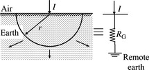
where ρe is average earth resistivity in Ωm and r is hemisphere radius. The arrows represent the diffusion of current through the earth. For example, for ρe = 100 Ωm and r = 1 m, RG ≈ 15.9 Ω.
If the sphere is buried at a depth of h in m which is large compared to twice its radius, the resistance to earth is given by
One driven vertical rod
Driven earth rods are generally solid and circular and are effective in small area substations or where low soil resistivity strata, into which the rod can penetrate, lies beneath a layer of high soil resistivity. The resistance to earth of a single isolated earth rod driven vertically into earth, shown in Figure 10.4, is given by

where L and r are the length and radius of the rod in m, respectively. For example, for a driven rod in an 11 kV substation with L = 3 m, r = 0.01 m and ρe = 100 Ωm,
Where the vertical electrode is surrounded by an infill material such as semi-conductive concrete or cement, the earth resistance is given approximately by
where ρi is resistivity of infill material in Ωm, ri is radius of shell of infill material in m and rrod is the radius of the rod in m. The resistivity of concrete infill material lie in the range of 30–90 Ωm.
Multiple driven vertical rods in a hollow square
Figure 10.5 shows multiple driven vertical rods in parallel arranged in a hollow square with adjacent rods being equally spaced. The equivalent resistance to earth of the combined rods is given by

where RG is the resistance of a single isolated rod given in Equation (10.11), N is the number of rods along each side of the square, d is the distance between adjacent rods in m and λ(N) is a factor that depends on the number of rods along each side of the hollow square. British Standard BS EN 7430:1998 Table 3 gives the value of λ as a function of N where X = 2.71 for N = 2, λ = 7.9 for N = 10 and λ = 9.4 for N = 20. For example, using the previous example rod data, N = 20 and d = 10 m, we obtain
Buried horizontal strip or wire
Horizontal strip or round wire conductor electrodes are very useful where high resistivity earth layer underlies shallow surface layers of low resistivity. The resistance to earth of a single strip or round wire conductor, shown in Figure 10.6, is given by

 (10.14)
where k = 1 for a strip conductor and k = 1.3 for a round wire conductor, L is length of strip or wire in m, h is depth in m and w is width of strip or diameter of round wire in m. For example, for a round wire conductor with L = 50 m, h = 0.5 m, w = 0.02 m and ρe = 100 Ωm, we obtain

Buried vertical or horizontal flat plate
Vertical or horizontal flat plate electrodes have large surface area and are used in soils where it is difficult to drive rods or where soil resistivity is very high. The resistance to earth of a buried vertical or horizontal flat plate, shown in Figure 10.7, is given by
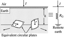
where h is depth to plate centre in m, r is the radius of an equivalent circular plate in m and is given by
where A is area of plate in m2.
For example, for a 1.1 m × 1.1 m plate buried at a depth of 1 m in a soil having

If the plate is placed on the surface of the earth, h = 0 and RG = 50/(4 × 0.62) = 20.2 Ω.
Buried horizontal ring of wire
The resistance to earth of a buried horizontal ring, shown in Figure 10.8, is given by
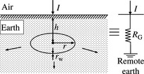
where r is radius of ring in m, h is depth in m and rw is radius of wire in m. For example, for ρe = 100 Ωm, r = 0.5 m, h = 0.5 m and rw = 0.01 m,
Buried horizontal grid or mesh
Figure 10.9 illustrates a horizontal grid or mesh system where RG represents the equivalent resistance to remote earth and Rm represents the local conductor resistance within the mesh.

The mesh is generally buried at a depth of 0.3−1 m. The resistance of the metal conductors forming the mesh is generally negligible compared to the resistance of the volume of earth in which the mesh is buried. The resistance to earth of a buried grid or mesh, is given by
where ![]() in m and A is area of mesh in m2.
in m and A is area of mesh in m2. ![]() is sum of lengths of buried conductors. For example, for a large 400 kV/132 kV substation with a 171 m × 171 m square mesh that consists of 20 × 20 conductor rods at 9 m intervals buried in a soil having ρe = 100 Ωm,
is sum of lengths of buried conductors. For example, for a large 400 kV/132 kV substation with a 171 m × 171 m square mesh that consists of 20 × 20 conductor rods at 9 m intervals buried in a soil having ρe = 100 Ωm, ![]() ,
, ![]() = (20 × 171) × 2 = 6840 m and
= (20 × 171) × 2 = 6840 m and
Combined horizontal mesh with driven vertical rods around periphery
Using Figure 10.10, the total equivalent resistance of an earthing system that consists of a combination of horizontal mesh and vertical rods electrodes is given by

where RG(mesh) and RG(N) are as given in Equations (10.17) and (10.13), respectively, RMut is a mutual resistance and is given by
where L is length of driven vertical rod in m and w is width of strap in m. For example, from the previous mesh and multiple vertical rods, RG(mesh) = 0.274 Ω and RG(N) = 2.36 Ω. For w = 0.05 m, the mutual resistance is
Therefore, the total equivalent resistance is
In this example, REq is practically equal to RG(mesh). Thus, the buried horizontal mesh is by far the most effective earth electrode and the additional vertical rods have introduced negligible improvement.
10.4 Overhead line earthing network
10.4.1 Overhead line earth wire and towers earthing network
Most high voltage lines and generally all extra high voltage lines have one or more earth wires. The earth wire is usually bonded to the tower top and connected to the earth meshes of substations where the line terminates. Terminal towers of lattice steel structures and poles of metallic construction are usually bonded to the substation earth electrode system. The line’s earth wire, as seen from the substation earthing system, usefully serves to extend this earthing system beyond the substation due to the tower connections to earth via the tower footing resistances. Figure 10.11 illustrates a single-circuit overhead line with a single earth wire where ZS is the self-series impedance of the earth wire per span with earth return. A span is the distance between two adjacent towers and ZS can be calculated using Equation (3.19a). RT is the tower earthing or footing resistance with the impedance of the tower itself being negligible at power frequency. For homogeneous earth resistivity ρe and with only earth wires present, i.e. no counterpoise conductor, the tower earthing or footing resistance RT is given by

Figure 10.11 Illustration of overhead line earth wire and tower footing resistance network of a single-circuit overhead line
where r is the radius of an equivalent hemispherical electrode having the same earth resistance as the tower footing. This radius is in the order of 1–2 m for smaller towers and may be 6–10 m for large towers with multiple legs. For example, for a typical 275 kV tower used in England and Wales having an equivalent radius of 2.8 m, the tower footing resistance is equal to 5.7 Ω, for a 100 Ωm earth resistivity.
10.4.2 Equivalent earthing network impedance of an infinite overhead line
In order to calculate the equivalent impedance of the combination of the earth wire and tower footing resistances, the line or number of spans is assumed infinite. Using Figure 10.11, the earth wire per span and tower footing resistance can be represented as a ladder network that consists of an infinite number of series–parallel elements as shown in Figure 10.12(a).
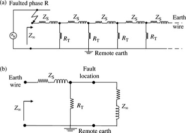
Figure 10.12 Equivalent earthing impedance of the infinitely long line shown in Figure 10.11: (a) ladder network representation of the earth wire and tower footing resistances and (b) derivation of equivalent impedance of a ladder network
Along the entire line length, the span lengths are assumed identical and the footing resistances of each tower are assumed equal. The tower at the fault location is not included in the equivalent circuit of the earth wire/tower footing. Assume that the driving point impedance of this ladder network as seen from the fault location is Z∞. Since the line is assumed infinitely long, the addition of one more series–parallel element does not change Z∞. This is illustrated in Figure 10.12(b) where
Solving this equation for Z∞, the practical solution is given by
 (10.21)
It is interesting to note that if ZS = RT then Z∞/RT = 1.6180 a number known since medieval times and related to the Fibonacci numbers which were first published in the Liber Abaci in 1202 AD. Equation (10.21) shows that the driving point impedance of this ladder network depends on the earth wire characteristics, e.g. material and size, tower footing resistance and earth resistivity along the line route. For example, consider a 132 kV single-circuit overhead line with a single aluminium conductor steel reinforced (ACSR) earth wire that has three spans per km and a self-impedance of (0.18 + j0.72)Ω/km. The tower footing resistance RT = 10 Ω. The driving point or ladder equivalent impedance is equal to

In practice, the line length beyond which the driving point impedance remains nearly constant is not infinite. This is discussed in the next section.
10.5 Analysis of earth fault ZPS current distribution in overhead line earth wire, towers and in earth
In this analysis, we use the single-circuit overhead line of Figure 10.11 and consider a one-phase to earth short-circuit fault at the terminal tower, numbered 0, as shown in Figure 10.13(a). We recall that ZS is the earth wire impedance in Ω/span.

Figure 10.13 Earth fault current distribution in earth wire, towers and earth of single-circuit overhead line: (a) earth fault current distribution in earth wire, towers and earth under a one-phase to earth short-circuit fault and (b) induced current circulating between towers
The fault current IF will divide between the terminal tower and the first span of the earth wire. The latter current will then flow into tower 1 and second span, and so on. Writing Kirchoff’s current law for towers or nodes n and (n − 1), we have
Writing Kirchoff’s voltage law for the nth earth wire span, we have
In Section 10.9, we will introduce the concept of a screening factor k for an overhead line with an earth wire but for now we will use the formula
Zm = (1 − k)ZS in Equation (10.23) to obtain
Similarly for the (n + 1)th earth wire span, we can write
Equation (10.24) suggests that the earth wire current i consists of two components: a variable component IC and a constant component Ii. The former is termed a conductive current that reduces with distance from the fault location as it progressively dissipates through the towers into earth. Ii is termed an inductive component because it is induced in the earth wire by the fault current IF flowing through the faulted phase conductor through the mutual impedance Zm between the faulted phase conductor and the earth wire. If IF is constant throughout the length of the line, Ii will also be constant throughout the length of the line as it effectively circulates within each span as illustrated in Figure 10.13(b). Now, substituting Equation (10.24) into Equation (10.22) and rearranging, we obtain
Also, substituting Equation (10.22) into Equation (10.24a), we obtain
Equations (10.25) are forward finite difference equations with a constant term in Equation (10.25b). It can be shown that the solution is given by
where A, B, a and b are constants and γ is the propagation constant and is given by
 (10.26c)
By substituting Equations (10.26) into Equation (10.22), we obtain
If the line is sufficiently long, the conductive current in the earth wire progressively dissipates through the towers to earth and becomes negligible at, say, tower n away from the fault location. Thus, substituting A = a = 0 in the varying terms of Equation (10.26a) and (10.26b), we obtain
Therefore, at the faulted terminal tower, n = 0, and for the first span, n = 1,
and the fault current at the faulted terminal tower, tower 0, is equal to
From Equations (10.29a) and (10.29b), we obtain
Substituting Equation (10.30) into Equation (10.28), we obtain
Equation (10.31) can be used to calculate the currents in any tower or earth wire span.
Using Equations (10.28a) and (10.29a), the conductive current in tower n is given by
where I0 is the conductive current in terminal tower 0. The tower number n, where the magnitude of the conductive current decays to a negligible value, say, 1.83% of the magnitude of I0 can be determined using Equation (10.32a). Thus,
 (10.32b)
If the remaining conductive current in tower n were chosen as 5% of I0, the constant ‘4’ in Equation (10.32b) changes to ‘3’. It is also of practical interest to determine the tower number n, or span number, and corresponding line length, where the tower conductive current drops to a negligible value of the sum of all tower conductive currents, denoted IC. Substituting n = 0, 1, 2,…, n in Equation (10.32a), and summing up all resulting tower currents, we obtain
Therefore, using Equation (10.33a), it can be shown that the tower number, or span number, n, where the tower current In = I0e−γn drops to 1.83% of IC is given by
where α = Real(γ), β = Imaginary(γ) and γ is given in Equation (10.26c). ZS is in Ω/span and RT is in Ω. The use of 1.83% is arbitrary but such a small value ensures a significant reduction in the nth tower current in per cent of IC. The line length that corresponds to such n towers or spans, given in Equation (10.33b), is given by
where Sp = 1/Np is the span length in km and Np is the number of spans per km.
To illustrate how the above equations may be used, consider the 132 kV overhead line of Section 10.4.2 that has three spans per km and ZS =(0.18 + j0.72)Ω/km. It is required to determine n and the corresponding line length where the conductive current drops to 1.83% of the total conductive current. Use a range of tower footing resistances of RT = 1, 10, 25, 50 and 100 Ω. For RT = 1 ω, we have

Similar calculations can be made for the remaining values of RT and the results are summarised in Table 10.1.
Table 10.1 Overhead line earthing network: propagation constant, tower number and line length where tower conductive current drops to 1.83% of total conductive current

Forthe given value of ZS, n and ![]() n saturate at around 28 and 9.3 km, respectively, as RT reaches 100 Ω. It is informative for the reader to calculate the variations in n and ln for ZS = (0.5 + j0.075)Ω/span.
n saturate at around 28 and 9.3 km, respectively, as RT reaches 100 Ω. It is informative for the reader to calculate the variations in n and ln for ZS = (0.5 + j0.075)Ω/span.
10.6 Cable earthing system impedance
Various methods of cable sheath/armour earthing arrangements were described in Chapter 3 and these depend on the cable rated voltage and the length of the cable. Like an overhead line’s earth wire, where the sheath/armour of cables are bonded to the substation earth electrode system, this serves to extend the effective area of the substation earthing system. A major portion of the earth fault current will normally return via the sheaths/armours of the cable supplying the fault current depending on the effectiveness of the sheath/armour earthing. A similar approach to that for an overhead line may be used to derive an equivalent earthing impedance for the cable sheath/armour where this is earthed allowing current circulation.
10.7 Overall substation earthing system and its equivalent impedance
The overall substation earthing system impedance consists of three main components. These are the substation earth electrode system, e.g. earth mesh or mat, the earth wire and tower footing network of overhead lines entering the substation, and the sheath/armour of cables emanating from the substation. In practice, where electrodes are spaced sufficiently far apart, it is normally sufficient to consider the component impedances to be in parallel as ‘seen’ from the substation as shown in Figure 10.14.

Figure 10.14 General extended substation earthing system: (a) components of substation earthing system and (b) substation equivalent earthing system impedance
Therefore, the overall substation earthing impedance with respect to remote earth is given by
 (10.34)
This impedance may be obtained by calculation at the design stage and confirmed by measurement.
10.8 Effect of system earthing methods on earth fault current magnitude
An earth fault current is a current that flows to earth and has a magnitude that depends on the method of system earthing. In solidly earthed and low impedance earthed systems, high levels of earth fault current result. However, earth fault currents are intentionally limited to very low levels in high impedance earthed systems. These systems may be earthed through a high impedance resistor or a high impedance reactor connected to transformer neutral points, or through the connection of an earthing or zig-zag transformer, sometimes with a neutral resistor, to systems supplied through delta-connected transformer windings. Industrial power systems tend to use low impedance earthing. Resonant earthing is where the system is earthed through a high impedance reactor called a Peterson coil, or arc suppression coil, i.e. usually connected to the neutral of distribution or zig-zag transformers. The variable impedance reactor is tuned to the overall system phase to earth capacitive reactance. In isolated systems, no intentional connection to earth is made but these systems are effectively earthed through the distributed capacitance of lines, cables and transformers windings. In both resonant earthed and isolated systems, the magnitude of earth fault current is very small. In effectively earthed systems, earth fault currents may be higher than three-phase fault currents.
10.9 Screening factors for overhead lines
We recall Figure 10.13 and Equation (10.31). The conductive current flowing through the first earth wire span away from the faulty terminal tower is considerably higher than those flowing in the spans further away from the fault. The conductive current flowing through the earth wire diminishes to zero as it dissipates through the towers to earth. The final value of the earth wire current in +1 in span (n + 1) is equal to the constant inductive current Ii, obtained from Equation (10.31b) by setting n → ∞,
It is important to note that this current, illustrated in Figure 10.13(b), does not enter earth and hence does not contribute to the rise of earth potential as will be seen later. From Figure 10.13(a) and starting from the faulted tower, we can write
where ![]() is the sum of all conductive or tower currents given in Equation (10.33a). From Figure 10.13, we observe that this current dissipates through the towers and return to the source through the earth. This current is therefore termed the earth return current and is given by
is the sum of all conductive or tower currents given in Equation (10.33a). From Figure 10.13, we observe that this current dissipates through the towers and return to the source through the earth. This current is therefore termed the earth return current and is given by
 (10.36b)
Thus, from Equations (10.35) and (10.36), we have
We are now ready to define the line’s screening factor using Equation (10.37b). This is defined as the ratio of the earth return current IER to the total fault current entering the earthing system at the fault location, i.e.
where the earth fault current entering the earthing system is IF = 3IZ and IZ is its zero phase sequence (ZPS) component. To express the line’s screening factor in terms of the line’s impedances, we assume that the line is sufficiently long so that the total earth wire impedance is large compared to the terminal resistances and we neglect the line shunt susceptance.
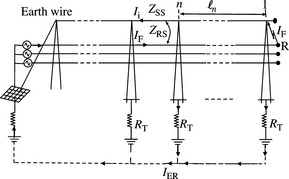
Figure 10.15 shows a line fed by a three-phase voltage source at the sending end and is open-circuited at the receiving end. When a single-phase short circuit occurs on phase R at the receiving end, the series voltage drop across one span of the faulted phase conductor and earth wire of length S in km beyond tower n is given by
 (10.39)
Therefore, from Equation (10.39), 0 = ZRSIF −ZSSIi or Ii = (ZRS/ZSS)/IF. Therefore, using Equations (10.37a) and (10.38), the line’s screening factor is given by
where ZSS is the self-impedance of the earth wire with earth return, and ZRS is the mutual impedance between the faulted phase conductor R and the earth wire with earth return. It is noted that Equation (10.40) can be rewritten as ZRS = (1 − k)ZSS which is the equation we used for Zm in Equation (10.23). The self and mutual impedances can be calculated using Equations (3.19a) and (3.20a), respectively, and are in Ω/km. From Equations (10.38) and (10.40), the earth return current IER and the earth wire inductive current Ii are given by
Equation (10.41a) shows that the screening factor k determines the proportion of the line’s earth fault current returning through earth at a distance greater than or equal to ![]() n where
n where ![]() n is given in Equation (10.33c). In addition, Equation (10.41a) suggests that in the absence of coupling between the faulted phase conductor and the earth wire, or in the absence of an earth wire, all the earth fault current returns to the source through the earth. The above analysis is also applicable to double-circuit overhead lines with one earth wire where ZRS now represents the mutual impedance between the faulted conductor phase R on one of the two circuits. The analysis method presented can be extended to calculate the screening factor for circuits with two earth wires. In England and Wales, for most 132,275 and 400 kV single-circuit and double-circuit overhead lines with one earth wire, the magnitude of k ranges from 0.60 to 0.75 i.e. 60–75% of the line’s phase fault current returns through earth and only 25–40% returns through the earth wire.
n is given in Equation (10.33c). In addition, Equation (10.41a) suggests that in the absence of coupling between the faulted phase conductor and the earth wire, or in the absence of an earth wire, all the earth fault current returns to the source through the earth. The above analysis is also applicable to double-circuit overhead lines with one earth wire where ZRS now represents the mutual impedance between the faulted conductor phase R on one of the two circuits. The analysis method presented can be extended to calculate the screening factor for circuits with two earth wires. In England and Wales, for most 132,275 and 400 kV single-circuit and double-circuit overhead lines with one earth wire, the magnitude of k ranges from 0.60 to 0.75 i.e. 60–75% of the line’s phase fault current returns through earth and only 25–40% returns through the earth wire.
10.10 Screening factors for cables
10.10.1 General
The current flowing in a single-core cable or the flow of unbalanced currents in the cores of a three-core cable induces voltages in the metallic sheath/armour of the cable. Under an earthed fault condition, and if the sheath/armour is earthed at each end, a current will circulate in the sheath/armour earth loop. This current is part of the earth fault current and the remaining part is the earth return current that returns through earth. The cable’s screening factor is dependent on the cable’s layout, earthing method, sheath/armour material, terminal earthing resistances and earth resistivity.
10.10.2 Single-phase cable with metallic sheath
Consider a single-phase cable with a metallic sheath but no armour having a length L in km. The cable is fed from a single-phase source at end 1 and subjected to a short-circuit fault at end 2 as shown in Figure 10.16(a). The cable core is denoted C and the sheath is denoted S and the latter is earthed at each end. The sheath terminal earthing resistances are denoted R1 and R2. Figure 10.16(b) shows the cable sheath earthing equivalent circuit. IF, IS and IER are the conductor fault current, sheath current and earth return current, respectively.

Figure 10.16 Calculation of screening factor for a single-phase cable with metallic sheath earthed at each end: (a) current distribution during a one-phase to earth short-circuit fault and (b) equivalent cable sheath circuit
The series voltage drop across the length of the conductor and sheath is given by
From Equation (10.42) and Figure 10.16, we have
Therefore, the cable’s screening factor is given by
The earth return current and sheath current are given by
The sheath current can be expressed as follows:
 (10.45)
As in the case of an overhead line, the current returning through the cable sheath consists of a conductive component and an inductive component given by
 (10.46a)
Ii is the inductive component of the sheath current due to inductive coupling between the core conductor and the sheath through the mutual impedance ZCS. IC is the conductive component of the sheath current due to conduction between the cable’s earthing terminals 2 and 1.
Equation (10.43) of the cable’s screening factor k includes the effect of the terminal earthing resistances. However, it is sometimes required to represent the effect of the cable parameters only. Therefore, with the terminal resistances set to zero, the cable’s screening factor is given by
Equation (10.47) can be rewritten using Equations (3.101a) and (3.103) as follows:
where RS(ac) is the sheath’s ac resistance and ZSS is given in Equation (3.101a).
It is interesting to note that the self-impedance of the faulted core conductor ZCC does not have any effect on the cable’s screening factor and hence on the current that returns through the sheath and also on the earth return current. Using IF = 3IZ, the earth return current and sheath current are given by
10.10.3 Three-phase cable with metallic sheaths
We presented in Chapter 3, a wide variety of three-phase cable circuit layouts and earthing arrangements. We will now illustrate the technique of calculating the cable’s screening factor for a general three-phase cable layout since the technique can be extended and applied to other layouts including armoured cables. Figure 10.17 illustrates a three-phase single-core cable having a length L in km and metallic sheaths, but no armour, and laid out in a flat symmetrical arrangement. At both ends of the cable, the sheaths are solidly bonded and connected to earth electrode where the terminal earthing resistances are denoted R1 and R2.

Figure 10.17 Calculation of screening factor for a three-phase single-core cable having a symmetrical flat arrangement and solidly bonded earthed sheaths: (a) current distribution during a one-phase to earth short circuit and (b) equivalent circuit of faulted cable conductor and sheaths
The cable is fed by a three-phase voltage source at end 1 and is open-circuited at end 2, the cable cores are denoted C1, C2 and C3, and the sheaths are denoted S1, S2 and S3. Under a single-phase to earth short-circuit fault on phase R, or conductor C1, at end 2, Figure 10.17(a) shows the resultant currents returning through the three sheaths and the current returning through earth. Figure 10.17(b) shows an equivalent circuit representation of the cable under this short-circuit fault condition. Using Equation (3.86), the series voltage drop across the cable, is given by
 (10.50a)
From Equation (10.50) and the symmetrical cable layout shown in Figure 10.17(a), we have ZS1S1 = ZS2S2 = ZS3S3 and ZS1S2 = ZS2S3. Thus, we can write
 (10.51a)
After some algebra, it can be shown that the cable’s screening factor is given by
 (10.52)
ZS1S1 is the self-impedance of sheath S1 with earth return, ZS1S2 is the mutual impedance between sheaths S1 and S2 with earth return, and ZS1S3 is the mutual impedance between sheaths S1 and S3 with earth return. ZC1S1, ZC1S2 and ZC1S3 are the mutual impedances between the faulted phase conductor R and sheaths S1, S2 and S3, with earth return, respectively. All impedances are in Ω/km. The self-impedance ZS1S1 can be calculated using Equation (3.101a) and all mutual impedances can be calculated using Equation (3.103).
For three-core cables and three single-core cables in a touching trefoil or equilateral layouts, the screening factor can be derived from Equation (10.52) by setting ![]() Thus,
Thus,
Substituting Equations (3.101a) and (3.103) into Equation (10.53), it can be shown that the cable’s screening factor is given by
 (10.54)
where RS(ac) is the sheath ac power frequency resistance, f is the nominal power frequency, d is the distance between the centres of cable phases, ris and ros are sheath inner and outer radii, and Derc is the depth of equivalent earth return conductor given in Equation (3.15).
Equations (10.52) and (10.53) of the cable’s screening factor k include the effect of the terminal earthing resistances R1 and R2, but if it is required to represent the effect of the cable parameters only, these resistances can be set to zero. However, the effect of the terminating resistances is important since they act to reduce the screening factor and hence the earth return current and increase the current that returns through the cable’s sheaths. Using IF = 3IZ, the earth return current and total sheath current are given by
As in the case of a single-phase cable, the sheath current IS consists of an inductive and a conductive component but we leave this simple derivation for the reader.
It is to note that in the case of three single-core cables of symmetrical flat formation, two different screening factors can be obtained. One would correspond to a short-circuit fault on the cable conductor laid in the central position and the other for a short-circuit fault on one of the cable conductors occupying an outer position. In our analysis here, we have considered the latter case. The derivation of the screening factor for the former case is straightforward using the method we have presented. Further, the method can be used to derive screening factors for cables having other physical layouts as well as armoured cables.
In most practical cable installations in medium, high and extra high voltage systems, and unlike overhead lines, the majority of the earth fault current for the fault conditions presented in this section returns through the cable sheaths and the rest through the earth.
10.11 Analysis of earth return currents for short-circuits in substations
Earth return currents are calculated under both single-phase and two-phase to earth short-circuit faults in substations. The calculation procedure and the current distribution under a solid one-phase to earth short-circuit fault in a substation is presented using a simple network of two substations separated by a single-circuit overhead power line with a single earth wire, as shown in Figure 10.18. The neutrals of the transformer star windings at the two substations are solidly connected to their respective substation earth electrode system. The overhead line earth wire is bonded to the earth mesh at both substations.
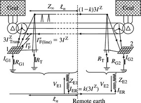
At substation 1, the initial rms phase fault current is the sum of the incoming phase fault currents on the line and the transformer and is given by
Since the phase fault current under a one-phase to earth fault is equal to three times the ZPS current, we have
At the short-circuit location, the short-circuit current supplied through the transformer returns to the substation transformer neutral, i.e. it circulates within the transformer. This current does not enter earth and as a result does not contribute to the earth return current and substation rise of earth potential. Based on the analysis presented in Section 10.5, part of the incoming earth fault current on the overhead line’s faulted phase will flow through the line’s earth wire and completely dissipates through the towers to earth at distance ![]() n from the fault location. At this distance, the current returning through the earth wire is the constant inductive current and that returning through earth is the earth return current. Using the line’s screening factor presented in Section 10.9, and I″F(line) = 3IZ, the earth return current at distance
n from the fault location. At this distance, the current returning through the earth wire is the constant inductive current and that returning through earth is the earth return current. Using the line’s screening factor presented in Section 10.9, and I″F(line) = 3IZ, the earth return current at distance ![]() n is given by
n is given by
and the earth wire inductive current is given by
where k is as given in Equation (10.40) and ![]() n is as given in Equation (10.33c).
n is as given in Equation (10.33c).
If the line length is shorter than ![]() n, the earth return current IER calculated by Equation (10.57a) will be an overestimate because in this case not all the conductive current returning through the earth wire would have dissipated through the towers to earth. Using Equation (10.34), the overall earthing impedance at the faulted substation with respect to remote earth consists of the parallel combination of the substation earth electrode resistance and the line’s earth wire/tower footing earthing impedance and is given by
n, the earth return current IER calculated by Equation (10.57a) will be an overestimate because in this case not all the conductive current returning through the earth wire would have dissipated through the towers to earth. Using Equation (10.34), the overall earthing impedance at the faulted substation with respect to remote earth consists of the parallel combination of the substation earth electrode resistance and the line’s earth wire/tower footing earthing impedance and is given by
10.12 Analysis of earth return currents for short circuits on overhead line towers
The calculation procedure of earth return current due to a short-circuit earth fault at a tower and the resultant current distribution in earth and line’s earth wire is presented using the simple network shown in Figure 10.19.
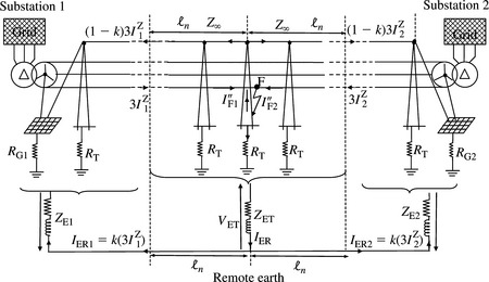
The initial rms phase fault current is the sum of the incoming phase fault currents on both sides of the tower and is given by
or rewritten in terms of their respective ZPS currents
At the faulted tower, part of the fault current flows into the earth through the faulted tower and its footing resistance. The other part flows into the earth wire in both directions away from the faulted tower. As in the analysis presented in Section 10.5, the currents carried by the earth wires of the first spans on both sides of the faulted tower are considerably higher than those flowing in the spans further away from the fault. After a distance equal to ![]() n in both directions, each earth wire current becomes constant and equal to the respective inductive current. Therefore, using the line’s screening factor k, the earth wire currents IS1 and IS2 and the earth return currents IER1 and IER2 at distance
n in both directions, each earth wire current becomes constant and equal to the respective inductive current. Therefore, using the line’s screening factor k, the earth wire currents IS1 and IS2 and the earth return currents IER1 and IER2 at distance ![]() n from the faulted tower are given by
n from the faulted tower are given by
For a short-circuit fault on the tower, the total earth return current that will cause a rise of earth potential at the tower base is given by
The overall earthing impedance at the faulted tower with respect to remote earth consists of the faulted tower footing resistance and the two earth wire ladder impedances in parallel as shown in Figure 10.20. Using Equation (10.34), the overall earthing impedance is given by

10.13 Calculation of rise of earth potential
Under normal unfaulted system conditions, the substation earthing system may have a potential that is slightly above that of remote earth of 0 V because on naturally unbalanced overhead lines, ZPS currents flow and return to the source via the substation earthing system. Also, the load in low voltage distribution networks may not be perfectly balanced. However, the design of the line and the degree of load unbalance usually ensure that these ZPS currents are kept low, so that the rise of earth potential with respect to remote earth is low and at safe levels.
During a single-phase to earth or two-phase to earth short circuits within a substation, large ZPS current flows through the earthing system in solidly earthed and low impedance earthed systems and this may cause a significant rise in earth potential depending on the magnitude of the effective substation earthing system impedance. In general, the electrode rise of earth potential with respect to remote earth system is given by
where ZE is given in Equation (10.34) and IER is the earth return current. In the case of an earth fault in a substation, as shown in Figure 10.18, the rise of earth potential at substation 1 with respect to remote earth using Equation (10.58), is given by
For an earth fault on a tower, as shown in Figure 10.19, the rise of earth potential at the tower with respect to remote earth, using Equation (10.63), is given by
Alternatively, using the tower fault current IT, the rise of earth potential at the tower with respect to remote earth can be calculated using Equation (10.20) as follows:
Where the tower fault current enters earth at the tower earthing electrode, the distribution of the current in the earth is non-uniform. However, the distribution becomes more uniform and radial after a small distance from the tower outside its earthing electrode. Therefore, the voltage on the surface of the earth with respect to remote earth at a distance x m from the edge of the tower earth electrode is given by the following approximate equation:
where VET is given in Equation (10.65), r is the equivalent radius of a sphere representing the tower earth electrode. Equation (10.66) can be used where the distance x is greater than twice the equivalent radius r.
10.14 Examples
Example 10.1
Consider the simple system of Figure 10.18. It is required to calculate the short-circuit earth return current and rise of earth potential at substation 1 for a single-phase to earth short-circuit fault in the substation.
The data for this system is as follows: a 50 Hz system and a 25 km 400 kV single-circuit overhead line with a single earth wire between substations 1 and 2.
| PPS (NPS) subtransient short-circuit infeed at 400 kV | 15 000 MVA |
| ZPS short-circuit infeed at 400 kV | 10 000 MVA |
| PPS and ZPS X/R ratios are assumed infinite for convenience in hand calculation | |
| Resistance of earth mesh electrode system | R1 = 0.1 Ω |
| PPS (NPS) subtransient short-circuit infeed at 400 kV | 32 000 MVA |
| ZPS short-circuit infeed at 400 kV | 35 000 MVA |
| PPS and ZPS X/R ratios are assumed infinite |
| PPS impedance | (0.017 + j0.3)/Ω/km |
| ZPS impedance | (0.12 + j0.82)/Ω/km |
| Earth wire self-impedance | (0.21 + j0.7)/Ω/km |
| Mutual impedance between faulted phase conductor and earth wire | (0.04 + j0.19)/Ω/km |
| Tower footing resistance | 10 Ω |
| Span length | 0.366 km |


Driving point impedance of infinite line

Substation 1 overall earthing impedance
The propagation constant is equal to
The tower number or number of line spans where the conductive current drops to 1.8% of the earth return current is equal to
The corresponding line length from the faulted substation is equal to ![]() n = 18 × 0.366 = 6.6 km.
n = 18 × 0.366 = 6.6 km.
To calculate the subtransient earth fault current, the Thévenin’s impedances at the point of fault are given by

The earth fault current, using IEC-60909 method and a voltage factor c = 1.1, is calculated as

The ZPS component of the earth fault current is calculated as
The ZPS current component supplied through the line is calculated as
The earth return current at a distance of 6.6 km from the fault location is given by
The earth wire current at a distance of 6.6 km from the fault location is calculated as
The rise of earth potential at substation 1 is calculated as
Example 10.2
Consider the simple system of Figure 10.19. It is required to calculate the short-circuit earth return current for a single-phase to earth short-circuit fault at a tower midway through the line. Calculate the rise of earth potentials at the tower and at 5 and 10 m distance from the edge of the tower earth electrode. Use the same data as in Example 10.1 and assume an earth resistivity of 100 Ωm.
To calculate the subtransient earth fault current, the Thévenin’s impedances at the faulted tower are calculated as follows:

Using IEC 60909 voltage factor c = 1.1, the tower earth fault current is equal to
The ZPS component of the tower earth fault current is calculated as
The ZPS current component supplied through the line from substation 1 is calculated as
The ZPS current component supplied through the line from substation 2 is calculated as
The earth return current flowing towards substation 1 calculated as
The earth return current flowing towards substation 2 is calculated as
The earth wire current at a distance of 6.6 km from the faulted tower on the side of substation 1 is calculated as
The earth wire current at a distance of 6.6 km from the faulted tower on the side of substation 2 is calculated as
The total earth return current is calculated as
The overall earthing impedance at the faulted tower is calculated as
The rise of earth potential at the faulted tower is calculated as
The equivalent radius for the tower’s earth electrode represented as a hemisphere is given by
Therefore, the required distances of 5 and 10 m are greater than 2r. The voltage on the earth’s surface at 5 m from the edge of the spherical earth electrode is
10.15 Electrical interference from overhead power lines to metal pipelines
10.15.1 Background
The proximity of overhead power lines, underground cables or traction lines to adjacent structures that have metallic parts such as communication cables, fences, surface or underground pipelines can produce harmful voltages in these structures. Our focus in this book is on the voltages produced in metal pipelines by overhead power lines. Metal pipelines are usually formed of steel tubes that are welded together and used for the transportation of various substances such as crude oil, natural gases, water, liquefied petroleum gases and sewage. The length of pipelines may range from several kilometres to hundreds or even thousands of kilometres. Most pipelines are usually buried at low depth although some may be installed above ground. Since the soil is electrolytic, ac corrosion of buried pipelines may occur when ac current is exchanged between the pipe and the earth. Therefore, buried pipelines have a few millimetre thick coating that insulates the metal from the surrounding earth and provides the primary protection against corrosion. New coatings include polyethylene and epoxy but for old pipelines, bitumen and glass cloth were used. Cathodic protection systems provide additional protection against ac corrosion. The technique consists of applying a low dc voltage along the pipe that negatively polarizes the metal with respect to earth thereby helping to minimise electrochemical corrosion of the metal by the soil. The risk of ac corrosion of pipelines begins at a much lower ac pipeline voltage than that which endangers safety. Generally, the ac voltage between the pipeline and a reference electrode above the pipeline should be less than 10 V if earth resistivity is greater than 25 Ωm but should not exceed 4 V if earth resistivity is less than or equal to 25 Ωm.
Metal pipelines are conductors that are generally insulated from earth. In proximity to overhead power lines, pipelines may be exposed to electrical interference for part of their length and this causes voltages to appear on the pipeline. Many countries specify maximum permissible touch voltages to protect pipeline workers. Under permanent or steady state conditions, maximum permissible touch voltages tend to range from 15 to 65 V. Under short duration fault conditions, the range is generally from 300 to 1500 V depending on short-circuit fault clearance times. In some countries, the limits are reduced if the public has access to the pipelines.
There are three types of electrical interference from power lines to pipelines. These are generally termed electrostatic or capacitive, electromagnetic or inductive, and resistive or conductive couplings.
10.15.2 Electrostatic or capacitive coupling from power lines to pipelines
Buried pipelines in proximity to overhead lines are not exposed to capacitive coupling from the power line because the earth acts as an electrostatic shield. Only pipelines installed above earth are subject to capacitive coupling from the conductors of overhead lines as illustrated in Figure 10.21(a). Where the pipeline runs physically in parallel with the conductors of the power line, the parallel exposure of the pipeline and power line is termed a parallelism. This is illustrated in Figure 10.21(b).

Figure 10.21 Illustration of electrostatic or capacitive coupling interference from a power line to a pipeline: (a) capacitive coupling and (b) parallel exposure
The coupling occurs under both normal and faulted power system conditions. The coupling causes voltages to appear on the insulated pipeline metal with respect to earth or currents to circulate in an earthed pipeline through the earthing connection. In general, voltage problems caused by capacitive coupling can be easily solved by earthing the pipeline. The pipeline voltages for a given pipeline exposure with the power line can be calculated using matrix analysis techniques as presented in Chapter 3. The self and mutual potential coefficients of the power line conductors are given in Equations (3.2a). Equation (3.2b) can also be used to calculate the mutual potential coefficients between the pipeline and the power line’s conductors where these form a parallelism. The self-potential coefficient of a pipeline close to the earth is given by
 (10.67)
where hp is the pipeline’s height above ground measured from the pipe’s centre and rp is the pipeline’s radius, both are in m. Recalling Equation (3.1) and writing it in partitioned matrix form for a multi-conductor system that consists of power lines and pipelines, we can write
 (10.68)
where C, p and E represent the power lines’ phase conductors, pipelines and power lines’ earth wires, respectively. The equation is general and allows for the presence of more than one power line with more than one earth wire and more than one pipeline. All potential coefficients in Equation (10.68) are matrices. The earthed earth wires are now eliminated by substituting VE = 0 in Equation (10.68), giving
 (10.69b)
The next step is to apply the pipelines’ earthing constraint to Equation (10.69a). For an insulated pipeline, Qp = 0 and, from Equation (10.69a), the pipelines’ voltages to earth due to capacitive coupling with the power lines are given by
where VC are the known phase voltages to earth of the power lines. If a person touches pipeline i whose voltage is Vp(i), the current that would flow through the person’s body is determined by the series combination of his contact resistance to earth and the pipeline’s capacitive reactance. In practice, the latter is much greater than the person’s resistance and therefore the discharge current is given by
and Li is length of pipeline exposed to capacitive coupling in km. If the pipelines are solidly earthed or earthed through a very low impedance, Vp = 0 and, from Equation (10.69a), we obtain
Since the phasor equivalent of the current i = dq/dt is I = jωQ, the pipelines’ charging currents are given by
The discharge current through the body of a person that touches pipeline i is given by
If the pipeline or some of its sections are not parallel to the power line, the distance between the pipeline, or a section of the pipeline, and the various power line conductors is no longer constant. Two such situations are illustrated in Figure 10.22. In both cases, the non-parallel pipeline exposure can be converted to a parallelism where the pipeline is parallel to the power line and is at an equivalent distance from the power line given by

Figure 10.22 Conversion of non-parallel exposures to parallel exposures between a power line and a pipeline: (a) oblique exposure near power line and (b) oblique exposure crossing power line
where xEq is the geometric mean distance to the power line and x1 and x2 are the minimum and maximum distances of the pipeline to the power line. The constraint of Equation (10.72b) is applied in order to maintain sufficient accuracy in calculating the mutual parameters between the pipeline and the power line. This constraint effectively places a limit on the length of a non-parallel pipeline section which necessitates dividing the pipeline into a number of sections each of which are converted to a parallel section to the power line.
For an insulated pipeline having a number of sections of both parallel and non-parallel exposures, the total pipeline voltage to earth can be calculated as the mean of the voltages in each section weighted by its length to the pipeline’s total length as follows:
 (10.73)
This voltage can be used to calculate the current that would flow through the body of a person that touches or comes into contact with the pipeline. The matrix analysis technique presented above can be extended and applied to double-circuit power lines.
10.15.3 Electromagnetic or inductive coupling from power lines to pipelines
General
Since the earth does not act as an electromagnetic shield, both above ground and buried pipelines in proximity to overhead lines are exposed to inductive coupling from the power line. The coupling exists under both normal steady state and faulted power system conditions and induces longitudinal voltages or electromotive forces (EMFs) on the pipeline. These EMFs produce voltage stresses on the pipeline and can also cause currents to circulate in the pipeline. These voltages (to earth) can reach several tens of volts under steady state conditions and a few kilovolts under fault conditions. The latter can damage the pipeline’s insulation coating and cathodic protection systems. The longitudinal induced EMF depends on the distance between the power line and pipeline and the length of parallelism. The inductive zone of influence of a power line increases with the earth’s resistivity and is generally taken as ![]() where y is in metres. For example, for
where y is in metres. For example, for ![]() The inductive coupling mechanism and zone of influence are illustrated in Figure 10.23 where the sections of the pipeline that fall within the zone of influence are AB, BC and CD. Each pipeline section presents an oblique exposure that can be converted to a parallelism using Equation (10.72).
The inductive coupling mechanism and zone of influence are illustrated in Figure 10.23 where the sections of the pipeline that fall within the zone of influence are AB, BC and CD. Each pipeline section presents an oblique exposure that can be converted to a parallelism using Equation (10.72).

Analysis of longitudinal induced EMFs on the pipeline
Mutual impedance between power line and pipeline
The EMF induced on a pipeline can be calculated under either normal steady state or faulted power system operating conditions. In both cases, the mutual impedances between the pipeline and the relevant power line conductors are required. Figure 10.24(a) illustrates the mutual inductive coupling between a single-circuit overhead power line with one earth wire and a buried pipeline parallel to the power line within the zone of influence.

Figure 10.24 Calculation of induced EMF on a pipeline from a power line: (a) illustration of mutual coupling between pipeline and power line, (b) induced EMF under normal operation and (c) induced EMF under fault condition
The mutual impedance between the pipeline p and an overhead line phase or earth wire conductor j, with earth return, is calculated using Equation (3.20a) as follows:
where dpj is the distance between the centres of the pipeline and line conductor j, f is system frequency and Derc is the depth of equivalent earth return given in Equation (3.15). If the distances between the pipeline and the power line’s conductors are greater than the distance given in Equation (3.20b), i.e. ![]() , Equation (10.74) results in an error that generally increases with distance particularly at low earth resistivity. The following equation gives an alternative formula for the mutual impedance and is valid for any distance between the pipeline and the power line:
, Equation (10.74) results in an error that generally increases with distance particularly at low earth resistivity. The following equation gives an alternative formula for the mutual impedance and is valid for any distance between the pipeline and the power line:
 (10.75)
The use of Equation (10.75) may result in a safe upper overestimate in the magnitude of the mutual impedance that is always lower than 8% provided that Equation (10.72) is used.
Induced EMFs during steady state unfaulted system conditions
In Figure 10.24(a), we consider a general case of a single-circuit overhead line with one earth wire. However, the analysis approach is general and applicable for more than one earth wire, double-circuit lines and underground cables. The phase and earth wire currents are illustrated in Figure 10.24(b). Each current induces a voltage on the pipeline through the appropriate mutual impedance between the pipeline and the conductor. Therefore, the total longitudinal EMF induced on the pipeline due to the three-phase currents and the earth wire current is given by
where the currents are in amps. The series voltage drop across the earth wire conductor is given by ![]() giving
giving
Substituting IE into Equation (10.76), we obtain
Equation (10.77) can be used whether the phase currents IR, IY and IB are balanced or not. If the power line has no earth wire, the ZpEIE term in Equation (10.76) disappears and the induced EMF is given by
Induced EMFs during a short-circuit fault in the power system
In many practical power systems, balanced three-phase short-circuit faults on high voltage power systems result in fault currents having a small degree of unbalance caused by the unbalanced network such as due to untransposed overhead lines. Therefore, the vector sum of the induced EMFs on an adjacent pipeline results in a small net induced EMF on the pipeline because the phase angle displacements between the three currents are not significantly different from 120°. The highest induced EMF on the pipeline will, therefore, occur under an unbalanced one-phase to earth short-circuit fault on the power system. The high ZPS current that flows on the power line induces a high EMF on a nearby pipeline depending on its proximity to the power line. Figure 10.24(c) illustrates a one-phase to earth short-circuit fault on phase conductor B, i.e. the nearest phase to the pipeline. The fault location is assumed at one extremity of the parallelism. For a fault within the length of the parallelism, the net EMF is calculated as the vector sum of the EMFs due to the opposing fault currents within the parallelism. From Figure 10.24(c), the series voltage drop across the earth wire is given by ![]() or
or ![]() The EMF induced on the pipeline is given by
The EMF induced on the pipeline is given by ![]() and using
and using ![]() we obtain
we obtain
and k is the screening factor. Equation (10.79b) is similar to Equation (10.40) except that the screening factor now includes the effect of both the earth wire and pipeline. Equation (10.79a) shows that since the fault current is constant within the parallelism, the longitudinal EMF per km induced on the pipeline will also be constant.
Analysis of pipeline voltages caused by inductive coupling
The calculation of pipeline voltages caused by the EMFs produced by inductive coupling from the power line, where the pipeline is within an overhead line’s zone of influence, requires the modelling of the pipeline and determination of its electrical characteristics. Like the conductors of an overhead transmission line, a metallic pipeline can be considered as a long lossy transmission conductor of known geometrical dimensions and physical characteristics. The magnetic coupling from the power line to the pipeline may be represented as distributed induced EMF sources on the pipeline. The equivalent circuit of a distributed pipeline section of length L in parallel with the conductors of an overhead power line is shown in Figure 10.25. E(x) is the induced EMF increment from the power line per km, z and y are the pipeline’s series impedance and shunt admittance per km and ZA and ZB are the impedances of the pipeline seen from ends A and B, respectively.

Figure 10.25 Equivalent circuit of a distributed metal pipeline inductively coupled to a power line: (a) pipeline section parallel to a power line and (b) pipeline distributed parameter equivalent circuit
From Figure 10.25(b), we can write
Differentiating Equations (10.80b) and (10.81b) with respect to x and using the original equations, we obtain
γ is the propagation constant of the lossy pipeline. Under normal unfaulted power system operation, the load currents influencing the parallel pipeline section are constant. The current will also be constant under a one-phase to earth fault condition on the power line beyond the section parallel to the pipeline. Under both conditions, the induced EMF is constant, i.e. E(x) = Eo. It can be shown that the solutions of Equations (10.82a) and (10.82b) are given by
 (10.83a)
 (10.83b)
Zo is the characteristic impedance of the lossy pipeline. Equation (10.83a) can be used to calculate the pipeline voltage to earth along the pipeline section, i.e. at any value of x between zero and L and Equation (10.83b) can be used to calculate the pipeline current. The terminal impedances ZA and ZB are chosen to represent the pipeline’s electrical characteristics at ends A and B of the pipeline section. For a pipeline section that continues for a few kilometres beyond end A, the electrical continuity of the pipeline persists and the pipeline’s impedance seen from point A may be taken as equal to the pipeline’s characteristic impedance or ZA = Zo. If the pipeline is solidly earthed at end A then ZA = 0 but if the pipeline has insulating joints and unearthed at end A, then ZA = ∞. These characteristics apply equally to end B. The magnitude of the pipeline voltage will obviously vary from zero, where the pipeline is earthed to a maximum where the pipeline is insulated and unearthed. For the case where the pipeline parallel section is insulated and unearthed at end B but extends beyond end A, i.e. ZA = Zo and ZB = ∞, Equations (10.83a) and (10.83b) simplify to the following:
The maximum pipeline voltage to earth occurs at end B, i.e. x = L and is given by
and the current at end B is I(x = L) = 0. At end A, i.e. x = 0, Equation (10.84a) gives
Beyond end A where the pipeline extends away perpendicular to the power line, the attenuation of the pipeline voltage can be evaluated to ensure that appropriate safety measures are taken to protect personnel working on the pipeline even many kilometres away. Using Equation (10.85b) that gives the pipeline voltage at end A, the pipeline voltage along a new axis a at a distance u beyond end A is given by
Where the pipeline extends beyond end A and remains inductively coupled to the power line, this can be considered a new pipeline section having an oblique exposure and converted to a parallelism using Equation (10.72).
Electrical characteristics of metal pipelines
Series impedance with earth return
In calculating the pipeline voltage to earth, we represented the pipeline as a long lossy distributed parameter conductor or transmission line. The pipeline was characterised by its propagation constant and characteristic impedance given in Equations (10.82c) and (10.83c), respectively, where z and y are the pipeline’s series impedance with earth return and shunt admittance. The series impedance consists of the internal impedance and external impedance with earth return. For pipelines installed above ground, the series impedance with earth return is given by
 (10.87)
where rp is the pipeline’s outer radius, μp is the relative permeability of the pipeline’s metal, typically about 300 for steel, ρp is the pipeline’s resistivity, f is the power frequency and Derc is as given in Equation (3.15). For buried pipelines, the external impedance part of the series impedance is dependent on the soil’s electrical characteristics and is a complicated function of the propagation constant γ. For computer-based calculations, the series impedance of a buried pipeline is given by
 (10.88)
where ![]() in m, is the equivalent radius of the pipeline, dp is the depth of the pipeline, ρe and εe are earth’s resistivity and permitivity, respectively. In Equation (10.88), γ should be in m−1. Generally, for modern buried coated pipelines, Equation (10.87) is found to be sufficiently accurate.
in m, is the equivalent radius of the pipeline, dp is the depth of the pipeline, ρe and εe are earth’s resistivity and permitivity, respectively. In Equation (10.88), γ should be in m−1. Generally, for modern buried coated pipelines, Equation (10.87) is found to be sufficiently accurate.
Shunt admittance
For an uncoated pipeline installed above ground at a height hp in m, the shunt admittance y = j2πfCp is calculated using Equations (10.67) and (10.70c). Thus
 (10.89)
where hp is measured from the pipe’s centre. For a coated and buried pipeline, its equivalent shunt admittance y consists of the coating’s admittance yc in series with the external earth admittance ye and is given by
 (10.91b)
where ρc is the resistivity of the pipeline’s coating in Ωm, εc is the coating’s relative permittivity and tc is the coating’s thickness in m. For coated pipelines with usually high coating resistivity, ye is much greater than yc and Equation (10.90) gives
10.15.4 Resistive or conductive coupling from power systems to pipelines
In Sections (10.11)-(10.13), we discussed how ZPS earth return currents due to short-circuit earth faults in substations and on overhead line towers cause a rise of earth potential with respect to remote earth over a given area. If a buried pipeline is located in the zone of influence, i.e. earth potential rise, irrespective of whether the pipeline is parallel to the power line or not, the coating insulation will be exposed to a voltage stress since the pipeline’s metal remains at virtually earth potential. If this voltage stress is greater than the dielectric strength of the insulation coating, it may puncture the coating and damage cathodic protection systems. If the pipeline passes through the earth electrode systems of substations or overhead power line towers, the voltage stress may be so high that it may puncture the coating. The intense leakage current may damage the pipeline’s metal. If the pipeline is earthed and connected to the earth electrode of a substation or tower, the rise of earth potential of the substation or tower will be transferred to the pipeline and may endanger safety.
10.15.5 Examples
Example 10.3
Consider a single-circuit 400 kV overhead transmission line with one earth wire and an above ground insulated metal pipeline in the vicinity as shown in Figure 10.26.
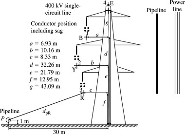
Figure 10.26 Power line and above ground pipeline for calculation of capacitive coupling for Example 10.3
The geometrical and physical data of the overhead line circuit is identical to that used in Example 3.4 and system frequency is 50 Hz. The pipeline is parallel to the axis of the power line at a distance of 30 m, has an outer radius of 0.35 m and its height above ground is 1 m. The length of parallel exposure of the pipeline and power line is 4 km. The three-phase voltages on the power line are in a balanced steady state condition. Calculate the touch voltage to earth on the pipeline induced by capacitive coupling with the power line and the discharge current that can flow through a person’s body when touching the pipeline.
The pipeline’s self-potential coefficient and mutual potential coefficients with the power line are

The potential coefficient matrix of the power line and pipeline coupled system is


As discussed in Section 10.2.3, a steady state current higher than about 5 mA would generally be considered unacceptable from personnel safety viewpoint. Therefore, the pipeline in this example would generally be earthed through an appropriate resistance typically of the order of a few hundred ohms.
Example 10.4
Consider a single-circuit overhead power line and a parallel metal pipeline in the vicinity. The power line carries a balanced set of three-phase steady state currents. Derive an expression for the induced EMF on the pipeline in terms of the distances between the pipeline and the power line’s phase conductors. Consider a power line with and without one earth wire.
We start with case where the power line has no earth wire. The balanced three-phase currents are PPS only thus IR = IP, IY = h2IP and IB = hIP. Therefore, from Equation (10.78), we have −EMFp = (ZpR + h2ZpY + hZpB)IP. Using Equation (10.74),

where the mutual impedances are in Ω/km and IR = IP is in amperes.
If the line has one earth wire, using Equation (10.77), and by analogy with the above equation, we obtain

Example 10.5
Consider the single-circuit 400 kV overhead transmission line of Example 10.3 and a non-parallel buried coated steel pipeline in the vicinity as shown in Figure 10.27. The pipeline is insulated and unearthed at end B and extends perpendicular to the overhead power line at end A.
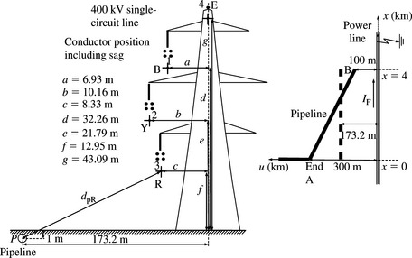
Figure 10.27 Power line and buried coated steel pipeline for calculation of inductive coupling for Example 10.5
The geometrical and physical data of the pipeline is as follows:
Outer radius = 0.25 m, depth = 1 m, resistivity and relative permeability of steel are 0.138 μΩm and 300, respectively. Insulation coating is polyethylene with thickness = 5 mm, resistivity = 25 × 106 Ωm and relative permittivity = 5.
Earth resistivity is 100 Ωm. System frequency is 50 Hz. Balanced steady state currents on the power line of 2000 A rms. One-phase to earth short-circuit fault current on phase R at the edge of zone of influence is 13 000 A rms.
Calculation of mutual impedances
The non-parallel pipeline is converted to a parallel pipeline at a geometric mean distance from the power line equal to ![]() . The zone of influence of the power line is
. The zone of influence of the power line is ![]() . Hence, the pipeline is well within the zone. The depth of earth return is
. Hence, the pipeline is well within the zone. The depth of earth return is ![]() . The distances between the pipeline and the power line’s phase and earth wire conductors are
. The distances between the pipeline and the power line’s phase and earth wire conductors are ![]() , similarly dpY = 164.63 m, dpB = 169.56 m and dpE = 178.72 m. The mutual impedances with earth return between the pipeline and the power line’s conductors are
, similarly dpY = 164.63 m, dpB = 169.56 m and dpE = 178.72 m. The mutual impedances with earth return between the pipeline and the power line’s conductors are


Electrical characteristics of the pipeline
The pipeline’s shunt admittance is

The series impedance of the pipeline with earth return is
The pipeline’s propagation constant is
The pipeline’s characteristic impedance is

Steady state unfaulted power system operation
The balanced three-phase currents are PPS only thus IR = 2000 A, IY = 2000 Ae−j2π/3 and IB = 2000 Aej2π/3. The induced EMF on the pipeline is

Therefore, EMFp = −16.7 − j8.32 = 18.66∠ − 153.5° V/km. If the overhead power line had no earth wire, the induced EMF is EMFp = -3.57 − j0.182 = 3.57∠−177.1° V/km. It is interesting to note that the effect of the power line’s earth wire under steady state conditions is to increase the induced voltage on the pipeline. This is opposite to the effect under fault conditions as shown in Equation (10.79).
The pipeline voltage to earth along the pipeline between ends A and B as well as beyond end A can be calculated using Equation (10.84a) between ends A and B and Equation (10.86) beyond end A where Eo = (−16.7 − j8.32)V/km and γ = (0.05525 + j0.06295)km−1. The maximum pipeline voltage at end B at x = 4 km is equal to −62.95 − j22.4 = 66.8∠ −160.4° V and the voltage at end A at x = 0 is equal to 4.82 + j8.83 = 10.06∠61.37° V.
One-phase to earth short-circuit fault condition
The overhead line’s screening factor is

The induced EMF on the pipeline is −EMFp = ZpRIFk or

Pipeline voltage to earth and pipeline current
We now calculate the profile of the pipeline voltage to earth along the pipeline between ends A and B as well as the attenuation beyond end A using Equations (10.84a) and (10.86) respectively. We also calculate the pipeline current along the pipeline between ends A and B using Equation (10.84b). In these Equations Eo = (−446.5 − j1117.5)V/km, γ = (0.05525 + j0.06295)km−1 and Zo = (5.478 + j3.11)Ω. The results of |V(x)| and |I(x)| are shown in Figure 10.28.

Figure 10.28 Calculated voltages to earth and current profiles on a steel pipeline inductively coupled to a 400 kV power line under a one-phase to earth fault condition. Corresponding to Figure 10.27
[1] Sunde E.D. Earth Conduction Effects in Transmission Systems. New York: Van Nostrand, Dover Publications; 1968.
[2] Tagg G.T. Earth Resistance. London: G. Newnes; 1964.
[3] DD IEC/TS 60479-1:2005, Effects of Current on Human Beings and Livestock—Part 1: General Aspects.
[4] British Standard BS 7430:1998, Code of Practice for Earthing.
[5] . Engineering Recommendation S34. A Guide for Assessing the Rise of Earth Potential at Substation Sites. London: Electricity Network Association; 1986.
[6] IEEE Standard 80:2001. Design of Power System Grounding.
[7] British Standard BS EN 12954:2001, Cathodic Protection of Buried or Immersed Metallic Structures-General Principles and Applications for Pipelines.
[8] Thapar B., et al. Evaluation of ground resistance of a grounding grid of any shape. IEEE Transaction on Power Delivery. April 1991;Vol. 6(No. 2):640-647.
[9] No. 2Nahman J., et al. Earth fault currents and potential distribution in composite systems. IEE Proceedings Generation Transmission and Distribution. Vol. 142. March 1995:135-142.
[10] Sverak J.G., et al. Safe substation grounding part 1. IEEE Transactions on PAS. September 1981;Vol. PAS-100(No. 9):4281-4290.
[11] Sverak J.G., et al. Safe substation grounding part II. IEEE Transactions on PAS. October 1982;Vol. PAS-101(No. 10):4006-4023.
[12] Endrenyi J. Analysis of transmission tower potentials during ground faults. IEEE Transactions on PAS. October 1967;Vol. PAS-86(No. 10):1274-1283.
[13] Verma R., Mukhedkar D. Ground fault current distribution in substation, towers and ground wire. IEEE Transactions on PAS. May/June 1979;Vol. PAS-98(No. 3):724-730.
[14] Dawalibi F.P. Ground fault current distribution between soil and neutral conductors. IEEE Transaction on PAS. March/April 1980;Vol. PAS-99:452-461.
[15] Popovic L.M. Determination of reduction factor for cable lines consisting of three single-core cables. IEEE Transactions on PD-18. 2003(No. 3):736-743.
[16] Taflove A., et al. Prediction method for buried pipeline voltages due to 60 Hz AC inductive coupling, Part I: Analysis. IEEE Transactions on PAS. May/June 1979;Vol. PAS-18(No. 3):780-794.
[17] Djogo G., Salama M.M.A. Calculation of inductive coupling from power lines to multiple pipelines and buried conductors. Electric Power Systems Research. 1997;Vol. 41:75-84.
[18] Dawalibi F.P., et al. Analysis of electrical interference from power lines to gas pipelines—Part 1: Computation methods. IEEE Transactions on Power Delivery. July 1989;Vol. 4(No. 3):1840-1846.
[19] Kouteynikoff P. Results of an international survey on the rules limiting interference coupled into metallic pipelines by high voltage power systems. Electra. No. 110(January 1987):55-66.
[20] Favez, B. and Gougeuil, J.C., Contribution to studies on problems resulting from the proximity of overhead lines with underground metal pipelines, Report No. 336. CIGRE, Session 1966.
[21] Wait J.R. Mutual coupling between grounded circuits and the effect of thin vertical conductor in the earth. IEEE Transaction on Antennas and Propagation. July 1983;Vol. AP-31(No. 4):640-644.
[22] Carson J.R. Wave propagation in overhead wires with ground return. Bell System Technical Journal. 1926;Vol. 5:539-554.
[23] Pollaczek F. Ueber das feld einer unendlich langen wechsel stromdurchflossenen einfachleitung. Electrishe Nachrichten Technik. 1926;Vol. 3(No. 9):339-359.
[24] Schelkunoff S.A. The electromagnetic theory of coaxial transmission lines and cylindrical shells. Bell System Technical Journal. 1934;Vol. XIII:532-578.
[25] Haberland G. Theorie der Leitung von Wechselstrom durch die Erde. Zeitschrifi fir Angewandte Mathematik und Mechanik. 1926(No. 6):366.