
5 Modelling of ac rotating machines
5.1 General
The short-circuit performance of ac rotating machines in power systems is of fundamental importance in the analysis of short-circuit currents and hence the safety of people and reliability of power systems. The modelling of rotating machines presents, in general, one of the most complex problems in the analysis of power systems. Fortunately, however, the required modelling detail of rotating machines depends on the type of study to be undertaken. In practice, different models are developed and used for load flow, short circuit, dynamic or electromechanical analysis and three-phase electromagnetic transient analysis, etc. The eventual aim of this chapter is to present the modelling of rotating machines in the sequence frame of reference for use in short-circuit analysis of power systems. However, in order to obtain an insight into the behaviour of rotating machines during transient fault conditions, the well-known machine model in the dq0 axis reference frame will be briefly presented and the machine models in the sequence frame of reference will then be derived. The presentation of the machine model in the dq0 reference is important since it provides an understanding of the meaning and origin of machine parameters, such as the machine d and q axes reactances and time constants, that can affect the short-circuit fault current.
Until the end of the twentieth century, almost all of the world’s electric power supply was virtually produced by synchronous generators. With emerging concerns over climate change and the need for reduced CO2 emissions, renewable energy, particularly using energy, is now becoming a main stream source of electric energy. Wind turbines utilising a range of novel non-synchronous generators are being used as a major new energy source in Western Europe (Denmark, Germany, Spain, UK, Holland, Ireland, etc.), North America (the US and Canada) and Asia (India and Japan). Wind farms that consist of tens to hundreds of wind turbine generators with individual turbine sizes of up to 5 MW are being built and turbine sizes in excess of 6 MW are under development and field testing. In addition to traditional synchronous and induction machines, short-circuit modelling of these new and emerging machines including those that utilise power electronics converters will also be described. The reader is expected to have a basic understanding of the theory of ac rotating machines.
5.2 Overview of synchronous machine modelling in the phase frame of reference
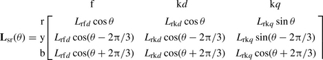
A brief overview of synchronous machine modelling in the phase frame of reference is presented. This model is a prerequisite to the derivation of the dq0 machine model as well as to the process of transformations from one reference to the other. The basic structure of a salient two-pole three-phase synchronous machine is shown in Figure 5.1(a) and a schematic is shown in Figure 5.1(b) illustrating stator and rotor circuits. The machine comprises three windings, r, y, b on the stator displaced by 120°; a field winding f that carries the direct current (dc) excitation and a short-circuited damper winding k on the rotor. The rotor can be cylindrical or salient pole in construction with the former mainly used in steam power plant and confined to two or four poles turbo-machines. Salient-pole machines are mainly used in hydro plant and low speed plant in general, and can have more than 100 poles. From the basic theory of magnetic coupling between circuits, the self and mutual inductances between stator and rotor circuits are defined as shown in Figure 5.1(b).
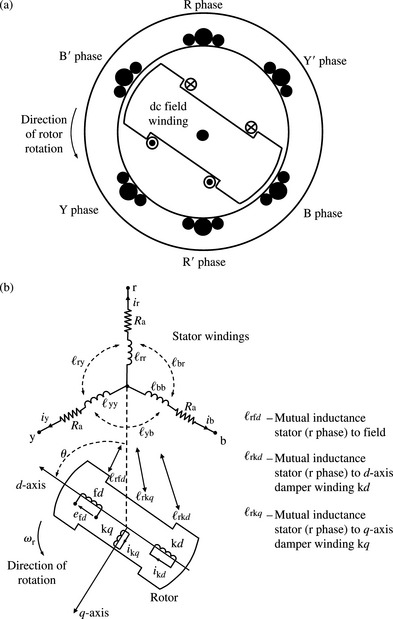
Figure 5.1 Three-phase salient-pole synchronous machine: (a) cross section and (b) illustration of stator and rotor circuits including mutual coupling
The damper winding is represented as two short-circuited windings; one in the same magnetic axis as the field winding f on the d-axis and termed kd and the other is a winding in an axis that is 90° ahead of the field axis and termed kq. We include one damper winding on the q-axis in our model. Figure 5.1(b) illustrates the field and damper windings on the rotor with respect to the d and q axes. The flux linkages in all six windings namely stator phases r, y and b, field winding f, damper windings k on d and q axes, using the generator convention, i.e. stator currents flowing out of the machine, are written in terms of self and mutual inductances as follows:

 (5.2c)
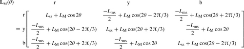
Lσ is stator leakage inductance and Lms is stator magnetising inductance. The expressions LM cos[f(θ)] in Equation (5.2a) represent the fluctuating part of the stator self and mutual inductances caused by the magnetically unsymmetrical structure of the rotor of a salient-pole machine. For a symmetrical round rotor machine, LM = 0. The subscripts rfd, rkd and rkq in Equation (5.2b) denote mutual inductances between stator winding phase r, and rotor field, d-axis damper and q-axis damper windings, respectively.
The zeros in the rotor inductance matrix Lrr represent the fact that there is no magnetic coupling between the d and q axes because they are orthogonal, i.e. displaced by 90°. If the machine were a static device such as a transformer, then all inductances in Equation (5.1) would be constant. However, as can be seen in Figure 5.1(b), because of the rotation of the rotor, the self-inductances of the stator winding and the mutual inductances between the stator and the rotor windings vary with rotor angular position. This is defined as θ = ωrt, where ωr is rotor angular velocity, and is the angle by which the d-axis leads the magnetic axis of phase r winding in the direction of rotation.
The stator and rotor voltage relations, i.e. for all six windings are given by
 (5.3)
(5.3)The zeros on the left-hand side of Equation (5.3) represent the short-circuited damper windings. The inductances of Equation (5.2) show that the flux linkages of Equation (5.1), and also the voltages of Equation (5.3) are non-linear functions of rotor angle positions. Generally, with the exception of studies of three-phase electromagnetic transients and sub-synchronous resonance analysis, this modelling is rather unwieldy and impractical for use in large-scale multi-machine short circuit, load flow or electromechanical stability analysis.
5.3 Synchronous machine modelling in the dq0 frame of reference
5.3.1 Transformation from phase ryb to dq0 frame of reference
The inductances of Equations (5.2a) and (5.2b) are time varying through their dependence on rotor angle position. Thus, the flux linkages are also functions of rotor angle position as given by Equation (5.1). Using Equation (5.2) in Equation (5.1), the rotor d and q axes damper winding flux linkages are given by
Equations (5.4a) and (5.4b) show a pattern involving the stator currents and rotor position. The outcome is new currents which can be expressed as follows:
It can be shown that the constant multiplier in Equation (5.5) is arbitrary and the choice of 2/3 results in the peak value of id being equal to the peak value of the stator current. A third variable can be conveniently defined as the zero sequence current which is ![]() . Therefore, the transformation from the stator ryb reference frame to the dq0 reference frame, written using stator currents, is given as
. Therefore, the transformation from the stator ryb reference frame to the dq0 reference frame, written using stator currents, is given as
 (5.7a)
 (5.7b)
 (5.7c)
The transformation matrix M−1(θ) allows us to transform quantities from the ryb reference frame to the dq0 reference frame, and vice versa using matrix M(θ). This transformation method with the frame of reference fixed on the rotor applies to the stator fluxes, voltages and currents, and is generally known as Park’s transformation.
This transformation process produces a new set of variables associated with two fictitious d and q stator windings that rotate with the rotor such that the stator inductances become constants as seen from the rotor during steady state operation.
Therefore, applying the transformation matrices of Equations (5.6a) and (5.6b) to Equation (5.1), and after much matrix and trigonometric analysis, we obtain
 (5.8a)
Similarly, we apply the transformation matrices of Equations (5.6a) and (5.6b) to the stator voltages of Equation (5.3) and note that the matrix M(θ) is derivable because its elements are functions of time through the rotor angular position. Therefore, after much trigonometric analysis, we obtain
 (5.9)
(5.9)5.3.2 Machine dq0 equations in per unit
The equations derived so far are in physical units. However, the analysis is greatly simplified by if they are converted into a per-unit form. Several per-unit systems have been proposed in the literature but we will use the equations that correspond to the system known as the Lad base reciprocal per-unit system. In this system, the pu mutual inductances among the three-stator field and damper windings are reciprocal and all mutual inductances between the stator and, field and damper windings, in the d and q axes are equal thus
Dropping the explicit pu notation for convenience, it can be shown that Equations (5.8a) and (5.9) can be written in pu form as follows:
 (5.11a)
 (5.11b)
In this pu system, we note that time is also in pu where tBase = 1/ωBase = 1/(2πfBase) with ΩBase =314.159 rad/s for a 50 Hz system. Also, since any reactance, e.g. Xd(Ω) = ΩLd = 2πfLd and XBase (Ω) = ΩBaseLBase = 2πfBaseLBase, it follows that if the stator frequency is equal to the base frequency, i.e.f = fBase, then
that is the pu values of Xd and Ld are equal. It is interesting to note that pu Equations (5.11a) and (5.11b) retain the same form as the physical ones, but the factor 1.5 has been eliminated from the rotor flux equations. Equations (5.11a) can be substituted in Equation (5.11b) and the result can be visualised using the simplified d and q axes equivalent circuits shown in Figure 5.2.

Figure 5.2(a) shows that the machine’s d-axis equivalent circuit, ignoring stator resistance, consists of a field winding resistance and reactance in series with a voltage source efd, a damper winding resistance and reactance, a mutual reactance and a stator leakage reactance. Figure 5.2(b) shows the q-axis machine equivalent circuit. This is similar to that of the d-axis except that there is no field winding on the q-axis.
5.3.3 Machine operator reactance analysis
In order to gain an understanding of the origins of the various machine parameters, e.g. subtransient and transient reactances and time constants, we will use the method of operator d and q axes reactances for its simplicity and the clear insight it provides.
q-axis operator reactance
We will take the Laplace transform of the stator and rotor flux linkages of Equation (5.11a) remembering that Laplace ![]() and s = jω. Also, we replace the inductance symbol L by the symbol X for reactance since pu inductance and pu reactance are equal. It is also convenient to express the variables in terms of changes about the initial operating point in order to remove the terms that correspond to the initial condition that is δf(s) = f(s)-f(0)/s. Thus
and s = jω. Also, we replace the inductance symbol L by the symbol X for reactance since pu inductance and pu reactance are equal. It is also convenient to express the variables in terms of changes about the initial operating point in order to remove the terms that correspond to the initial condition that is δf(s) = f(s)-f(0)/s. Thus
Taking the Laplace transform of the q-axis damper voltage equation, last row of Equation (5.11b), and rearranging, we obtain
Substituting Equation (5.14a) into Equation (5.13b) and rearranging, we obtain
Substituting Equation (5.14b) into Equation (5.13a) and rearranging, we obtain
where the q-axis operator reactance is defined as Xq(s) and is given by
d-axis operator reactance
Taking the Laplace transform of the first, fourth and fifth rows of Equation (5.11a),
 (5.16a)
Also, taking the Laplace transform of the fourth and fifth rows of Equation (5.11b),
By substituting δ ψfd(s) and δ ψkd(s) from Equation (5.16a) into Equation (5.16b), we solve for δifd(s) and δikd(s) in terms of δefd(s) and δid(s). We then substitute this result back into Equation (5.16a), and use Equation (5.12), we obtain, after some algebra
where the d-axis operator reactance Xd(s) is given by
5.3.4 Machine parameters: subtransient and transient reactances and time constants
q-axis parameters
Using Equation (5.12), we can rewrite the q-axis operator reactance of Equation (5.15b) as follows:

 (5.20c)
are the q-axis open-circuit and short-circuit subtransient time constants. We note that we divided these time constants by ωs to convert from pu to seconds.
These time constants could also be derived by inspection from Figure 5.3(a). In the case of the open-circuit time constant, the equivalent reactance seen looking from the q-axis damper winding with the machine terminals open-circuited is Xkq in series with Xaq. This is then divided by the q-axis damper winding resistance Rkq to obtain the time constant. In the case of the short-circuit time constant, the equivalent reactance seen looking from the q-axis damper winding with the machine terminals short-circuited is Xkq in series with the parallel combination of Xaq and Xσ. This is then divided by the q-axis damper winding resistance Rkq to obtain the time constant.

Figure 5.3 Machine parameters from its equivalent circuits: (a) q-axis: subtransient and steady state equivalent circuits and (b) d-axis: subtransient, transient and steady state equivalent circuits
The effective machine q-axis reactance at the instant of an external disturbance is defined as the subtransient reactance X″q. Using Equation (5.20a), this is given by
Substituting Equations (5.20b) and (5.20c) into Equation (5.21a) and using Equation (5.12), we obtain after some algebra
 (5.21b)
Again, the above q-axis subtransient reactance could be derived by inspection from Figure 5.3(a) with Rkq = 0 because the rotor flux linkages cannot change instantly following a disturbance. This is equivalent to looking into the machine from its q-axis terminals. This shows Xσ is in series with the parallel combination of Xaq and Xkq.
In the absence of a disturbance or under steady state conditions, the effective machine q-axis reactance is defined as the synchronous reactance Xq. Using Equation (5.20a)
It should be noted that using the q-axis operator reactance of Equation (5.20a), no q-axis transient time constant or transient reactance are defined and the latter can be assumed equal to the steady state value. This is due to our use of one q-axis damper winding on the q-axis as shown in Figure 5.2(b). This representation is accurate for laminated salient-pole machines and still reasonably accurate for a round rotor machine is sometimes that represented as two parallel damper winding circuits on the q-axis. In the latter case, the second may sometimes be used to represent the body of the solid rotor.
The q-axis operator reactance of Equation (5.20a) can be expressed in terms of partial fractions as follows:
 (5.21d)
d-axis parameters
Following extensive algebraic manipulations, we can show that Equation (5.18a) can be written in the following form:
 (5.22b)
The numerator and denominator of Equation (5.22a) can be expressed in terms of factors as follows:
T′do and T″do are the transient and subtransient open-circuit time constants
T′d and T″d are the transient and subtransient short-circuit time constants
Accurate expressions for the machine open-circuit and short-circuit time constants can be derived by equating the numerator of Equation (5.22a) with that of Equation (5.23a), and similarly for the denominators. However, such a procedure would involve the solutions of quadratic equations and the values of the open-circuit and short-circuit time constants would result in rather involved expressions in terms of the time constants of Equation (5.22b). Reasonable approximations can be made on the basis that the field winding resistance is much smaller than the damper winding resistance. This means that T2 (and T3) « T1 and T5 (and T6) « T4. Therefore, Equation (5.22a) can be written as
Therefore, from Equations (5.23a) and (5.23b), we have
The effective machine d-axis reactance at the instant of an external disturbance is defined as the subtransient reactance X″d. Using Equation (5.23a), this is given by
This can also be expressed in terms of the internal machine d-axis parameters using Equations (5.22b) and (5.23c), hence
The d-axis operator reactance after the decay of the currents in the damper winding following an external disturbance can be represented by setting Xkd = 0 and Rkd → ∞ in Equation (5.23b) and making use of Equation (5.23c). The result is given by
Equation (5.25a) in fact also represents the case of a machine with only a field winding on the rotor but no damper winding. The effective machine d-axis reactance at the beginning of a disturbance is now defined as the transient reactance X′d. Using Equation (5.25a), this is given by
This can also be expressed in terms of the internal machine d-axis parameters using Equations (5.22b) and (5.23c), hence
From Equations (5.24a) and (5.25b), the following useful expression can be obtained
In the absence of a disturbance or under steady state conditions, the effective machine d-axis reactance is defined as the synchronous reactance Xd. Using Equations (5.23a) or (5.25a)
Again, the d-axis subtransient and transient time constants and reactances as well as the steady state reactance can be calculated by inspection from Figure 5.3(b).
The d-axis operator reactance of Equation (5.23a) can be rewritten as follows:
This expression can be approximated to a sum of three partial fractions assuming that T″d and T″do are small compared with T′d and T′do. The result is given by
Equation (5.27) describes the machine reactance variation in the s domain as given in both IEC and IEEE standards for synchronous machines.
5.4 Synchronous machine behaviour under short-circuit faults and modelling in the sequence reference frame
Having established the machine d and q axes operator reactances, we are now able to proceed with analysing the behaviour of the machine under sudden network changes such as the occurrence of balanced and unbalanced short-circuit faults. Our objective is to understand the nature of short-circuit currents of synchronous machines and in order to do so, it is important to understand the meaning of positive phase sequence (PPS), negative phase sequence (NPS) and zero phase sequence (ZPS) machine impedances.
5.4.1 Synchronous machine sequence equivalent circuits
In Section 5.3, we defined the machine reactances and time constants in the dq0 reference frame. In short-circuit analysis, the machine PPS, NPS and ZPS machines models or equivalent circuits need to be defined as well as the sequence reactances. The three-phase synchronous generator is designed to produce a set of balanced three-phase voltages having the same magnitude and displaced by 120°. As we have already seen in Chapter 2, the transformation of these balanced three-phase voltages into the sequence reference frame produces a PPS voltage source in the PPS network but zero voltages in the NPS and ZPS networks. The stator windings of the machine are usually star connected and the neutral is usually earthed through an appropriate impedance. The earthing is usually used to limit the machine current under a single-phase short-circuit terminal fault to the rated current of the machine. We designate the machine PPS, NPS and ZPS reactances as XP, XN and XZ, respectively. The machine PPS, NPS and ZPS equivalent circuits are shown in Figure 5.4 with the sequence quantities being those that correspond to phase r. As expected, the neutral earthing impedance appears only in the ZPS equivalent circuit and is multiplied by a factor of 3. The values of the sequence reactances and resistances is discussed in the next sections.

5.4.2 Three-phase short-circuit faults
Short-circuit currents
Before the occurrence of the short circuit, the machine is assumed in an open-circuit steady state condition and the rotor speed is the synchronous speed ωs. The field voltage and current are constant, the damper currents are zero and the armature phase voltages are balanced three-phase quantities. Let t = 0 be the instant of short circuit that occurs at the machine terminals and let θo be the angle between the axis of phase r and direct axis at t = 0. Thus, θo defines the point in the voltage waveform at which the short-circuit occurs. The following initial conditions just before the short circuit, using Equations (5.11a) and (5.11b), are obtained
 (5.28a)
We assume that, during the short-circuit period, the machine rotor speed and field voltage remain constant. The latter assumes no automatic voltage regulator (AVR) action. Therefore, immediately at the instant of the short circuit, we have
Remembering that δf(s) = f(s) − f(0)/s, the stator d- and q-axis voltages in Equation (5.11b), transformed into the Laplace domain and using Equations (5.28), can be written as follows:
Using Equation (5.28a), Equation (5.15a) becomes
Using Equations (5.28), Equation (5.17a) becomes
Substituting Equations (5.30a) and (5.30b) into Equations (5.29a) and (5.29b), and rearranging, we obtain
Solving Equations (5.31a) and (5.31b) for d and q axes stator currents, we obtain
We will make a number of simplifications that help us to obtain the time domain solution of the d and q axes stator currents of Equation (5.32). From Equation (5.32b)
 (5.33a)
 (5.33b)
Ta is the stator or armature short-circuit time constant and is divided by ωs to convent it from pu to seconds and Ra is the stator de resistance. In arriving at Equation (5.33a), we made two approximations which, in practice, would have a negligible effect. First, we ignored R2a/[Xd(s)Xq(s)] because it is too small in comparison with ω2s. We then added 1/(Ta)2 where 1/(Ta)2 « ω2s. We also replaced Xd(s) with X″d, and Xq(s) with X″q in the term that multiplies sRa because we assumed that the rotor field and damper winding resistances are very small. This means that the factors (1 + sT) in Equations (5.20a) and (5.23a) can be replaced with sT. Therefore, substituting Equation (5.33a) into Equations (5.32a), we obtain
Substituting Equations (5.21d) and (5.27) into Equations (5.34) and taking the inverse Laplace transform, it can be shown that the time domain d and q axes currents are given by
 (5.35a)
The stator or armature phase r current can be calculated by transforming the d and q axes currents into the phase frame of reference using Equations (5.6a) and (5.6b) and noting that under balanced conditions io = 0. Therefore, using θ = ωst + θo, ir(t) = id(t)cos θ-iq(t)sin θ, and after much trigonometric analysis, we obtain
The currents in the two stator phases iy(t) and ib(t) are calculated with θo replaced by θo - 2π/3 and θo + 2π/3, respectively.
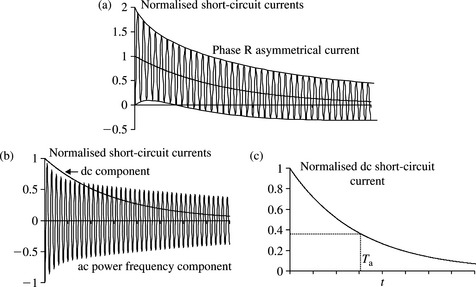
Equation (5.36) represents the total phase r current following a sudden three-phase short circuit fault at the machine terminals with the machine initially unloaded but running at rated speed. The short-circuit current contains three main components; a power frequency (e.g. 50 or 60 Hz) component, a transient unidirectional or dc component and a transient double-frequency (e.g. 100 or 120 Hz) component. Both the dc component and the double-frequency component decay to zero with a time constant equal to Ta which is typically between 0.1 and 0.4 s. These current components are illustrated in Figure 5.5.
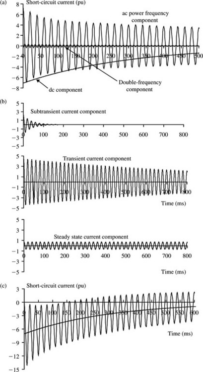
Figure 5.5 Three-phase short-circuit fault at a synchronous machine terminals: (a) the three components of the short-circuit current, (b) the three subcomponents of the ac power frequency component and (c) phase r short-circuit asymmetrical current
The initial magnitude of the dc component is dependent on the instant of time at which the short circuit occurs, i.e. θo and therefore the initial magnitudes of the dc components in the three phases are different but they all decay at the same rate given by the time constant Ta. The dc component in each phase appears in order to satisfy the physical condition that the current cannot change instantaneously at the instant of fault. The initial value of the transient double-frequency component is small as it is due to the difference between the d and q subtransient reactances (X″q - X″d); an effect termed as subtransient saliency. This current component disappears if the d and q subtransient reactances are equal. This component is neglected in network short-circuit analysis.
The power frequency component itself consists of three subcomponents as shown in Equation (5.36) and illustrated in Figure 5.5(b). These are termed the subtransient, transient and steady state components. The subtransient component decays to zero with a time constant T″d and typically lasts for up to 0.15 s. The transient component decays much more slowly to zero with a time constant T′d and typically lasts for up to 5 s. The steady state or sustained component is constant. The parameters of the machine that determine the magnitude and rate of decay of each current component are the various reactances and short-circuit time constants shown in Equation (5.36). The sum of the dc and power frequency ac components produces an asymmetrical short-circuit current waveform. The phase r asymmetrical current is illustrated in Figure 5.5(c).
PPS reactance and resistance
The three-phase short-circuit is a balanced condition resulting in balanced ac currents in the three phases of the machine. From Equation (5.36), we can express the instantaneous power frequency component of the short-circuit current as ir(t) = Real[Ir(t)] where Ir(t) is phase r complex instantaneous current given by
where ![]() is phase r complex instantaneous voltage and
is phase r complex instantaneous voltage and
is an equivalent time-dependent machine PPS reactance as shown in Figure 5.6.
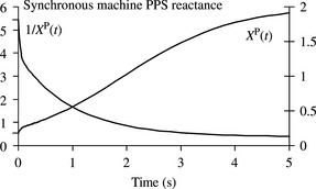
Figure 5.6 Synchronous machine time-dependent PPS reactance under a three-phase short-circuit at machine terminals
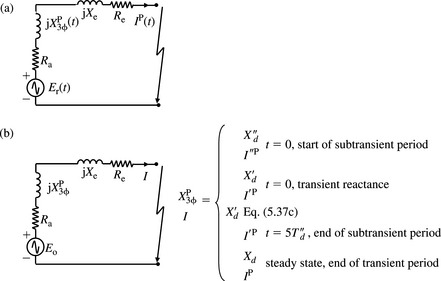
As presented in Chapter 2, the phase r complex voltage can also be written as Er(t) = Erejωst where Er is complex phasor given by ![]() . As in the case of instantaneous currents, the complex phase y and phase b currents Iy(t) and Ib(t) are obtained by replacing θo of Ir(t) with θo - 2π/3 and θo + 2π/3, respectively. The complex instantaneous PPS current is given by Ip(t) = [Ir(t) + hIy(t) + h2Ib(t)]/3 = Ir(t). Figure 5.7(a) shows the machine PPS equivalent circuit with a time-dependent equivalent reactance. We define such an equivalent circuit as a transient PPS symmetrical component equivalent circuit. Figure 5.7(b) shows the fixed impedance approach of the machine PPS reactance that is conventionally considered to consist of three components; subtransient, transient and steady state components. If a time domain short-circuit analysis technique is used, then Equation (5.37b) or Equation (5.36) can be used directly to calculate the machine reactance or current at any time instant following the occurrence of the fault. However, the vast majority of large-scale short-circuit analysis computer programs used in practice use fixed impedance analysis techniques and this will be discussed in Chapter 6. Essentially, different values of reactance are used to calculate short-circuit currents at different times following the instant of fault. At the instant of short-circuit fault, t = 0, i.e. the start of the subtransient period, Equation (5.37b) givesXp = X″d. Also, neglecting the subtransient current component, the value of the transient reactance at t = 0 is obtained by putting t = 0 in Equation (5.37b) giving Xp = X′d. The steady state reactance Xp = Xd applies from the end of the transient period when the transient current component has vanished, i.e. t ≥ 5T′d. Another machine PPS reactance, found useful in practice, is the reactance that applies at the end of the subtransient period, i.e. at t = 5T″d. Thus, using Equation (5.37b), this is given by
. As in the case of instantaneous currents, the complex phase y and phase b currents Iy(t) and Ib(t) are obtained by replacing θo of Ir(t) with θo - 2π/3 and θo + 2π/3, respectively. The complex instantaneous PPS current is given by Ip(t) = [Ir(t) + hIy(t) + h2Ib(t)]/3 = Ir(t). Figure 5.7(a) shows the machine PPS equivalent circuit with a time-dependent equivalent reactance. We define such an equivalent circuit as a transient PPS symmetrical component equivalent circuit. Figure 5.7(b) shows the fixed impedance approach of the machine PPS reactance that is conventionally considered to consist of three components; subtransient, transient and steady state components. If a time domain short-circuit analysis technique is used, then Equation (5.37b) or Equation (5.36) can be used directly to calculate the machine reactance or current at any time instant following the occurrence of the fault. However, the vast majority of large-scale short-circuit analysis computer programs used in practice use fixed impedance analysis techniques and this will be discussed in Chapter 6. Essentially, different values of reactance are used to calculate short-circuit currents at different times following the instant of fault. At the instant of short-circuit fault, t = 0, i.e. the start of the subtransient period, Equation (5.37b) givesXp = X″d. Also, neglecting the subtransient current component, the value of the transient reactance at t = 0 is obtained by putting t = 0 in Equation (5.37b) giving Xp = X′d. The steady state reactance Xp = Xd applies from the end of the transient period when the transient current component has vanished, i.e. t ≥ 5T′d. Another machine PPS reactance, found useful in practice, is the reactance that applies at the end of the subtransient period, i.e. at t = 5T″d. Thus, using Equation (5.37b), this is given by

Figure 5.7 Synchronous machine PPS equivalent circuits for a three-phase short-circuit at machine terminals: (a) transient PPS time-dependent equivalent circuit and (b) fixed impedance equivalent circuits at various time instants
 (5.37c)
In summary, the four PPS reactances are given by
 (5.37d)
For typical salient-pole and round rotor synchronous machines, Equation (5.37c) shows that the PPS reactance at the end of the subtransient period is typically equal to 1.1X′d to 1.5X′d.
The stator or armature dc resistance Ra is very small. The PPS power frequency stator resistance includes, in addition to stator losses, hysteresis and eddy current losses and may be 1.5-2 times the stator dc resistance. The machine PPS equivalent circuit, depending on the calculation time period of interest, are shown in Figure 5.7(b).
Effect of short-circuit fault through an external impedance
In many practical situations, the location of short-circuit fault will be on the network to which the machine is connected either directly or through a dedicated transformer. Therefore, an equivalent impedance will be present between the machine and the fault location. The effect of such an external machine impedance, denoted (Re + sXe), and shown in Figure 5.8, is now considered.
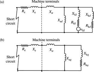
Figure 5.8 Three-phase short-circuit seen by a synchronous machine through an external impedance: (a) d-axis and (b) q-axis
The effect of the external impedance (Re + sXe) can be considered to be equivalent to modifying the stator leakage reactance and stator resistance as shown in Figure 5.8. The analysis is in fact identical to the previous case without an external impedance except that the operator reactances will need to be modified to include the external impedance (Re + sXe). Using Equation (5.32a) and (5.32b), it can be shown that

The direct analytical solution of these equations is very tedious. An alternative approach is to calculate the short-circuit current components individually by substituting the relevant reactances. For example, to calculate the subtransient, transient and steady state power frequency current components, we substitute X″d, X′d and Xd in place of ωsXd(s), and X″q and Xq in place of ωsXq(s). Without going through the long mathematical analysis, it can be shown that the phase r short-circuit current, ignoring the double-frequency component, is given by
 (5.38a)
As before, the other two stator phases iy(t) and ib(t) are obtained with θo replaced by θo - 2π/3 and θo + 2π/3, respectively. Similar to the case with no external impedance, it can be shown that the effective short-circuit time constants in Equation (5.38a) can be expressed in terms of the open-circuit time constants as follows:
 (5.38b)
 (5.38c)
 (5.38d)
Equation (5.38d) can be approximated, with insignificant loss of accuracy, to
Usually the stator and external resistances are much smaller than the reactances. Thus, the transient and subtransient time constants reduce to the following:
The effect of the external resistance Re should not be neglected in calculating the armature or dc time constant given in Equation (5.38e).
The PPS equivalent circuits of the machine, ‘seeing’ a short circuit through an external impedance, depending on the calculation time period of interest, are shown in Figure 5.9.
Simplified machine short-circuit current equations
For most practical short-circuit calculations, simplified short-circuit equations can be used assuming X″d = X″q. Assuming maximum dc current offset and ignoring the double-frequency component, the peak current envelope of Equation (5.36), at any time instant, is given by
In the case of a fault through a predominantly inductive external impedance, the peak current envelope of Equation (5.38a) at any time instant is given by
 (5.40b)
5.4.3 Unbalanced two-phase (phase-to-phase) short-circuit faults
Consider a two-phase or phase-to-phase short-circuit fault at the machine terminals involving phases y and b with the machine initially running at synchronous speed, rated terminal voltage and on open circuit. The initial conditions prior to the fault are given in Equations (5.28a) and (5.28b). The constraint equations that define the two-phase short-circuit fault are given by
Transforming Equation (5.41a) and (5.41b) to the dq0 reference using Equation (5.7b), we obtain
Equations (5.41c) to (5.41e) and the machine Equations (5.11) that relate currents to fluxes and rate of change of fluxes to voltages provide a set of equations that are sufficient to obtain the solution of currents under a phase-to-phase short-circuit fault at the machine terminals. However, the resulting current equations are complex and non-linear and a closed form solution is extremely tedious. Instead, a step-by-step simplification process, similar to that described for a three-phase fault, can be used. The short-circuit current can be shown to contain a power frequency component, a dc component and both even and odd harmonic orders of the power frequency, the latter due to subtransient saliency. However, for practical calculations of machine phase-to-phase short-circuit currents involving the power frequency and dc components only and neglecting the harmonic components, it can be shown that the phase y and b short-circuit currents are given by
 (5.42a)
XN is the machine NPS reactance.
The maximum dc current component in Equation (5.42a) occurs when θo = 0.
From Equation (5.42a), we can express the instantaneous power frequency component of the short-circuit current as iy(t) = Real[Iy(t)] where Iy(t) is phase y complex instantaneous current and is given by
 (5.44a)
is phase r complex instantaneous voltage, Er is phase r complex phasor given by
 (5.44b)
is an equivalent time-dependent machine PPS reactance. At the fault instant t = 0, i.e. start of subtransient period, Xp(2φ) = X″d + XN. At t = 0 and neglecting the sub-transient component, Xp(2φ) = X′d + XN. At t ≥ 5T′d(2φ), i.e. end of transient period, ![]() . The machine reactance at the end of the subtransient period, i.e. at t ≈ 5T″d(2φ) is given by
. The machine reactance at the end of the subtransient period, i.e. at t ≈ 5T″d(2φ) is given by
 (5.44c)
In summary, the four fixed machine reactances are given by
 (5.44d)
As we presented in Chapter 2, the transient PPS and NPS currents of the power frequency components of the complex instantaneous phase currents Iy(t) and Ib(t) of Equation (5.44a) can be calculated using
Substituting Equation (5.44a) into Equation (5.45a), we obtain
Figure 5.10(a) shows the resultant transient symmetrical component equivalent circuit that satisfies Equation (5.45b) with the reinstated machine stator resistance for completeness. Figure 5.10(b) shows equivalent circuits using the fixed reactances of Equation (5.44d). The time constants of Equation (5.42b) and (5.42c), and the time-dependent machine reactance of Equation (5.44b) show, from a PPS current view point, that under a two-phase short-circuit fault the machine behaves as if it has ‘seen’ a balanced three-phase short-circuit through an external reactance XN.

Figure 5.10 Synchronous machine equivalent circuits for a two-phase short-circuit fault at machine terminals: (a) transient PPS time-dependent equivalent circuit and (b) fixed impedance equivalent circuits of various time instants
NPS reactance and resistance
We return to the NPS reactance XN given in Equation (5.43b). This is the machine reactance that results from the flow of NPS stator currents. Let us first recall that during a balanced three-phase short-circuit, only PPS currents flow into the short circuit. These currents set up a MMF wave that rotates at synchronous speed in the same direction of rotation of the rotor. Because of the very high X/R ratio of the machine, the MMF wave lines up almost exactly with the d-axis hence d-axis currents only meet d-axis reactances. However, when NPS currents flow in the stator of the machine, these currents produce a MMF wave that rotates at synchronous speed in an opposite direction to the rotation of the rotor. It therefore rotates backward at twice synchronous speed with respect to the rotor. Thus, the currents induced in the rotor field and damper windings are double-frequency currents. At such a high frequency, the machine reactances are effectively the subtransient reactances and as the MMF wave sweeps rapidly over the d and q axes of the rotor, the equivalent NPS reactance alternates to d and q axes subtransient reactances. Therefore, the NPS reactance is defined, by both IEC and IEEE standards, as the arithmetic mean of the d and q axes subtransient reactances or
We have stated previously that when subtransient saliency is present, the short-circuit current will contain both even and odd harmonics. In this case, we have a different machine NPS reactance which is given by the geometric mean of the d and q axes subtransient reactances as shown in Equation (5.43b). However, because X″d and X″q are nearly equal, the difference between the arithmetic mean and the geometric mean is very small. The difference can be illustrated for both a round rotor machine and a salient-pole machine as follows. For a typical round rotor synchronous generator with X″d = 0.2 pu and X″q = 0.24 pu, their arithmetic and geometric means are 0.22 and 0.2191 pu, respectively. For a salient-pole machine with X″d = 0.18 pu and X″q = 0.275 pu, their arithmetic and geometric means are 0.2275 and 0.22248 pu, respectively. Given the uncertainty associated with the measurements of these quantities which can be up to 10%, differences in XN of less than 2.5% are generally acceptable.
XN takes the same value under subtransient, transient and steady state conditions as illustrated in Figure 5.10(b).
The stator NPS resistance is significantly higher (some 10–20 times) than the PPS resistance because the second harmonic backward rotating MMF causes significant additional I2R losses in the rotor circuits due to double frequency currents in the rotor field and damper windings. For short-circuit analysis, the use of Ra instead of the NPS resistance is conservative.
Simplified machine short-circuit current equations
For maximum dc current offset, the peak current envelope of Equation (5.42a) at any instant of time is given by
 (5.47)
5.4.4 Unbalanced single-phase to earth short-circuit faults
Consider a single-phase to earth short-circuit fault at the machine terminals involving phase r with the machine initially running at synchronous speed, rated terminal voltage and on open circuit. The machine neutral is assumed solidly earthed and the initial conditions prior to the fault are given in Equations (5.28a) and (5.28b).
The constraint equations that define the single-phase short-circuit fault are given by
Transforming Equation (5.48) to the dq0 reference using Equation (5.7b), we obtain
As in the case of a two-phase short-circuit, Equations (5.48) and (5.11) are sufficient to obtain the solution of current under a single-phase short-circuit fault at the machine terminals. However, the resulting current equations are complex and non-linear and a closed form solution is extremely tedious. Instead, a step-by-step simplification process, similar to that described for a three-phase fault can be used. The single-phase short-circuit current can be shown to contain, in general, a power frequency component, a dc component and both even and odd harmonic orders of the power frequency, the latter due to subtransient saliency. However, for practical calculations of machine single-phase short-circuit currents involving the power frequency and dc component only, neglecting the harmonic components, it can be shown that the phase r short-circuit current is given by
 (5.49a)
Equation (5.49a) shows that the magnitude of the dc component of short-circuit current is maximum when θo = π/2. In the time constant equations, XZ is the machine ZPS reactance. XN is the machine NPS reactance under a single-phase short-circuit fault condition and is given by
 (5.49e)
Since, X″d and X″q are nearly equal, then if we set X″d = X″q in Equation (5.49e), we obtain XN = X″d. Although the expression of Equation (5.49e) is different from the expressions given in Equations (5.43b) and (5.46), the difference in numerical values is practically insignificant.
From Equation (5.49a), we can express the instantaneous power frequency component of the short-circuit current as ir(t) = Real[Ir(t)] where Ir(t) is phase r complex instantaneous current given by
 (5.50a)
where ![]() is phase r complex instantaneous voltage, Er is phase r complex phasor given by
is phase r complex instantaneous voltage, Er is phase r complex phasor given by ![]() and
and
 (5.50b)
is the machine equivalent time-dependent machine PPS reactance under a single-phase short-circuit fault condition. At the fault instant t = 0, i.e. start of subtransient period, Xp(1φ), = X″d + XN + XZ. At t = 0 and neglecting the subtransient component, ![]() . At
. At ![]() . The machine reactance at the end of the subtransient period is given by
. The machine reactance at the end of the subtransient period is given by
 (5.50c)
In summary, the four fixed reactances are given by
 (5.50d)
The transient PPS, NPS and ZPS currents of the complex phase current Ir(t) of Equation (5.50a) are calculated using
Substituting Equation (5.50a) into Equation (5.51a), we obtain
Figure 5.11(a) shows the transient PPS equivalent circuit that satisfies Equation (5.51b) with the reinstated machine stator resistance for completeness. Figure 5.11(b) shows equivalent circuits using the fixed machine reactances of Equation (5.50d). The time constants of Equation (5.49) and the time-dependent machine reactance of Equation (5.50b) show, from a PPS current view point that, under a single-phase to earth short-circuit fault, the machine behaves as if it has ‘seen’ a balanced three-phase short-circuit through an external reactance equal to Xe = XN + Xz.
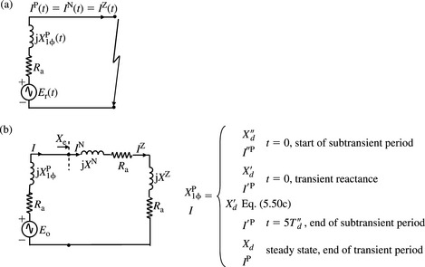
Figure 5.11 Synchronous machine equivalent circuits for a one-phase to earth short-circuit fault at machine terminals: (a) transient PPS time-dependent equivalent circuit and (b) fixed impedance equivalent circuits of various time instants
Figure 5.11 shows the resultant symmetrical component equivalent circuits with the machine PPS reactance connected in series with the machine NPS and ZPS reactances to satisfy the single-phase short-circuit fault condition.
ZPS reactance and resistance
The machine ZPS impedance to the flow of ZPS armature currents applies where the stator winding is star connected and the neutral is not isolated. Recalling the spacial distribution of the stator phases and that ZPS currents are equal in magnitude and phase, these currents produce no net power frequency MMF wave across the air gap. Therefore, the ZPS impedance to the flow of ZPS currents is only due to some stator winding slot leakage flux which is greatly dependent on the machine coil pitch design. The ZPS reactance is always smaller than the stator leakage reactance Xσ and may be less than half of it depending on coil pitch.
Since there is no power frequency stator MMF wave across the air gap, the ZPS reactance is independent of the rotor’s rotation. It is therefore constant and has the same value under subtransient, transient and steady state conditions as illustrated in Figure 5.11(b). The ZPS resistance can be assumed equal to the stator or armature ac resistance.
Simplified machine short-circuit current equations
For maximum dc current offset, the peak current envelope of Equation (5.49a) at any instant of time is given by
 (5.52)
5.4.5 Unbalanced two-phase to earth short-circuit faults
Consider a two-phase to earth short-circuit fault at the machine terminals involving phases y and b with the machine initially running at synchronous speed, rated terminal voltage and on open circuit. The machine neutral is assumed solidly earthed and the constraint equations that define the two-phase-to-earth short-circuit are given by
Transforming Equation (5.53) to the dq0 reference using Equation (5.7b), we obtain
As in the previous short-circuit cases, Equations (5.54) and (5.11) are theoretically sufficient to obtain the solution of currents under a two-phase to earth short-circuit fault at the machine terminals. However, the resulting equations are very complex and non-linear and a closed form solution is extremely unwieldy. Instead, a step-by-step simplification process can be used to derive the various components of the short-circuit currents. For practical calculations of machine short-circuit currents involving the power frequency and dc components only assuming that X″d = X″q it can be shown that the phase y and phase b short-circuit currents are given by
 (5.55a)
 (5.55b)
The earth fault current is the sum of phase y and phase b currents, hence
 (5.56a)
XN is the machine NPS reactance under a two-phase to earth short-circuit fault condition which, in the general case when X″d ≠ X″q, is given by
 (5.58a)
The limiting values, i.e. the lower and upper bounds of Equation (5.58a) can be found by letting XZ → 0 and XZ → ∞, respectively. Thus, XN is bound as follows
The lower limit is the same as that found in the case of a three-phase fault given in Equation (5.33b). Also, the upper limit is the same as that found in the case of a two-phase fault given in Equation (5.43b). In practice, the differences between the various expressions for XN, that depend on the short-circuit fault type, are negligible. The value of XN calculated from the arithmetic average of X″d and X″q given in Equation (5.46) is sufficiently accurate for practical short-circuit analysis purposes. It should be noted that if we let X″d = X″q in Equation (5.58a), we obtain, as we should expect, XN = X″d. Equations (5.55a) and (5.55b) of phase y and phase b short-circuit currents are quite different from those obtained for all short-circuit fault types considered previously. Each phase current now consists of two asymmetrical current components and each one of these consists of a power frequency ac component and a dc component. As expected, at t = 0, the sum of the ac and dc components of each asymmetrical current is zero. The earth fault current, on the other hand, consists of one asymmetrical current with only one power frequency ac component and one dc component as the other terms cancel out when the phase currents are added together. It is important to note that the two dc components have different initial magnitudes and different armature time constants.
The maximum dc offset occurs at θo = 0 for the first dc component but at θo = π/2 for the second dc current. It can be shown the value of θo that results in maximum asymmetrical phase y and phase b currents is given by
 (5.59a)
Typically X″d ≈ 2XZ hence at t = 0, θo(y) = −49.1° and θo(b) = 49.1°. Also, for a typical 50 Hz synchronous machine with X″d = 0.2 pu, XZ = 0.1 pu and Ra = 0.002 pu, the armature dc time constants calculated using Equation (5.57b) are Ta1(2φ-E) = 0.2122 s and Ta2(φ-E) = 0.318 s. Thus, using Equation (5.59a), we obtain θo(y) = -49.87°, (θo(b) = 49.87°) at t = 10ms and θo(y) = -53.1° (θo(b) = 53.1°) at t = 50 ms.
From Equation (5.56a) of the machine equivalent reactance under a two-phase to earth short-circuit, we distinguish four machine fixed impedance values. At t = 0, i.e the start of the subtransient period, Xp(2φ-E) = X″d + Xe. At t = 0, and neglecting the subtransient component, ![]() . At
. At ![]() , i.e. end of transient period,
, i.e. end of transient period, ![]() . The machine reactance at the end of the subtransient period, i.e. at
. The machine reactance at the end of the subtransient period, i.e. at ![]() , is given by
, is given by
 (5.59b)
In summary, the four fixed reactances are given by
 (5.59c)
From Equations (5.55a) and (5.55b), we can express the instantaneous power frequency component of the short-circuit currents as iy(t) = Real[Iy(t)] and ib(t) = Real[Ib(t)] where Iy(t) and Ib(t) are the phase y and phase b complex instantaneous currents given by
 (5.60a)
 (5.60b)
 (5.60b)
where ![]() and
and ![]() . The transient PPS, NPS and ZPS currents of the complex phase currents Iy(t) and Ib(t) of Equations (5.60) are calculated using
. The transient PPS, NPS and ZPS currents of the complex phase currents Iy(t) and Ib(t) of Equations (5.60) are calculated using
Substituting Equations (5.60a) and (5.60b) in Equation (5.60c), and using Equation (5.56b) for Xe with XN = X″d, we obtain, after some algebraic manipulations, which the reader is encouraged to prove, the following:
 (5.61b)
 (5.61c)
Figure 5.12(a) shows the transient PPS equivalent circuit that satisfies Equation (5.61a) with the reinstated stator resistance for completeness. Figure 5.12(b) shows equivalent circuits using the fixed machine reactances of Equation (5.59c). From Figure 5.12(b) and using complex phasor notation, the PPS phasor current is given by
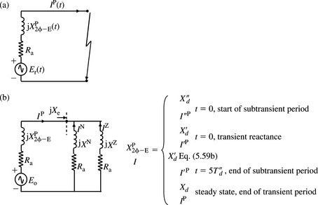
Figure 5.12 Synchronous machine equivalent circuits for a two-phase to earth short-circuit fault at machine terminals: (a) transient PPS time-dependent equivalent circuit and (b) fixed impedance equivalent circuits of various time instants
 (5.62a)
where the value of the PPS reactance XP is as shown in Figure 5.12(b) and depends on the calculation time instant. The NPS and ZPS phasor currents are given by
The machine equivalent reactance of Equation (5.56a) and the time constants of Equation (5.57a) show that from a PPS current view point under a two-phase to earth short-circuit fault, the machine behaves practically as if it has ‘seen’ a balanced three-phase short circuit through an external impedance Xe. This impedance is given by the parallel combination of the NPS and ZPS machine reactances given in Equation (5.56b).
5.4.6 Modelling the effect of initial machine loading
Machine internal voltages
The short-circuit current equations already presented cover all cases of short-circuit currents at the machine terminals assuming the machine is initially unloaded that is the internal machine rms voltage is equal to Eo. However, the equations can be slightly modified to represent the situation where the machine is initially loaded by accounting for its prefault active and reactive power outputs as well as its terminal voltage. Because the machine is initially only producing a balanced set of three-phase voltages into a balanced network, the NPS and ZPS terminal voltages and output currents are all zero. Similarly, the initial machine active and reactive power outputs are PPS MW and PPS MVAr quantities. Assuming that the initial machine terminal voltage, active and reactive power outputs are Vt, P and Q, the machine stator current I can be calculated using the apparent power equation P + jQ = VtI*. We have already established that the machine PPS reactance XP can be equated to one of four reactances depending on the calculation time instant after the occurrence of the fault. Therefore, using Figure 5.13, the internal machine voltages that correspond to these four reactances, for a given terminal voltage Vt, are E″, E′(at t = 0), E′(at t = 0), E′(at t ≈ 5T″d) and E, respectively, and are given by
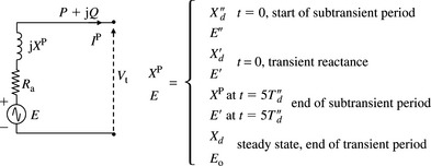
Clearly, when the machine is initially unloaded, I = 0 and E″ = E′ = E = Eo = Vt.
Machine short-circuit currents
Using Equations (5.63) for E″, E′(at t = 0) or E′(at t ≈ 5T″d) and E, the equations that describe the machine peak short-circuit current envelope for each fault type are given below.
Three-phase short circuit
Using Equation (5.40a) and neglecting the double-frequency component, we have
 (5.65)
 (5.66)
Two-phase to earth short circuit
In the ac components of Equations (5.55a) and (5.55b), we simply replace the term Eo/X(2φ−E)(t), using Equation (5.56a), with the following term
 (5.67)
In the dc components of Equations (5.55a) and (5.55), the term Eo should be replaced with E″.
5.4.7 Effect of AVRs on short-circuit currents
Discussion of the function, design, analysis or tuning of AVRs is the subject of power system dynamics, stability and control. In our book, we simply mention that the AVR generally attempts to control the machine terminal voltage by sensing its variations from a given set point or target and causing an increase or a decrease in the excitation or field voltage. In the case of short-circuit faults on the host network to which a synchronous machine is connected, the machine terminal voltage can see a significant drop during the fault period depending on the electrical distance, i.e. impedance to the fault point. The question we are interested in is what effect can the AVR have, if any, on the machine short-circuit current for a three-phase fault at the machine terminals from an unloaded initial condition? We recall that we have already determined the machine short-circuit current assuming no AVR action with δefd = 0. To determine the machine current due to a change in field voltage δefd, representing automatic AVR action, we recall Equation (5.17a), ![]() from which we obtain
from which we obtain
and from Equation (5.15a)
Equations (5.18a) for Xd(s) and (5.18b) for Gd(s) were derived for the general case of a machine with a damper winding. For a machine without a damper winding, a similar method can be used to derive these expressions and the reader is encouraged to do so. However, for us, we will directly derive the expressions for Xd(s) and Gd(s) from the general ones of Equations (5.18a), (5.18b) and (5.19a). To do so, we represent the absence of the damper winding by substituting Xkd = 0 and letting Rkd → ∞. After a little algebra, the results can be easily shown as
Substituting Equations (5.69a) and (5.69b) into Equation (5.68a) and using Xffd = Xfd + Xad and Xd = Xad + Xσ from Equation (5.12), we obtain
and Equations (5.22b) for T4 and (5.23c) for T′d, we obtain
For simplicity, we consider an instantaneous or a step change in field voltage δEfd where δEfd(s) = δEfd/s. Therefore, Equation (5.70a) can be written as
and taking the inverse Laplace transform, we obtain
Also, from Equation (5.68b), we have
Equation (5.70b) shows that an instantaneous increase in Efd causes an exponential increase in short-circuit current with a time constant equal to T′d(3φ). That is, despite the very fast change in Efd, the resultant change in machine current is slowed down or delayed by the d-axis short-circuit transient time constant T′d(3φ) which falls in the range of 0.5−2 s. For example, for a typical value of T′d(3φ) = 1 s, the factor ![]() is equal to 0.11 at 120 ms. This indicates some change in current towards the end of the subtransient period, i.e. at around t = 120 ms. However, in practice, even for modern fast excitation control systems such as brushless ac rotating exciters or static exciters, the change infield voltage will itself occur after a definite time delay. Thus, the effective change in short-circuit current will only begin to occur after the subtransient period. In practice, a static excitation control system will not be able to continue to operate by maintaining free thyristor firing if the terminal voltage, where it derives its supply, drops below around 0.2–0.3 pu. In other words, the subtransient component of short-circuit current will have decayed to zero by the time the effect of the AVR is felt through the machine. Therefore, the effect of the AVR is to cause a possible increase in the transient and steady state components of short-circuit current. It should be noted that the change in field voltage has no effect on the dc component of short-circuit current as shown in Equations (5.70b) and (5.70c).
is equal to 0.11 at 120 ms. This indicates some change in current towards the end of the subtransient period, i.e. at around t = 120 ms. However, in practice, even for modern fast excitation control systems such as brushless ac rotating exciters or static exciters, the change infield voltage will itself occur after a definite time delay. Thus, the effective change in short-circuit current will only begin to occur after the subtransient period. In practice, a static excitation control system will not be able to continue to operate by maintaining free thyristor firing if the terminal voltage, where it derives its supply, drops below around 0.2–0.3 pu. In other words, the subtransient component of short-circuit current will have decayed to zero by the time the effect of the AVR is felt through the machine. Therefore, the effect of the AVR is to cause a possible increase in the transient and steady state components of short-circuit current. It should be noted that the change in field voltage has no effect on the dc component of short-circuit current as shown in Equations (5.70b) and (5.70c).
We have now obtained the machine current changes due to both the short-circuit itself and the change in field voltage. Therefore, using the superposition theorem, the total machine short-circuit current change is obtained by the addition of the two values. Thus, examining the effect on the ac component of short-circuit current after the subtransient component has decayed to zero, Equation (5.35a) can be rewritten as
Therefore, using Equations (5.70b) and (5.71a), the total change in machine current is given by
A simplification can be made by using δEfd = Efd - Efdo and since the machine is initially unloaded, we have ![]() . Therefore, Equation (5.71b) simplifies to
. Therefore, Equation (5.71b) simplifies to
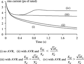
Equation (5.72) shows two transient components; one is a rising exponential and one is decaying exponential and both have the same time constant T′d(3φ). The decaying exponential component represents, as expected, the decay in flux due to induced currents in the field winding whereas the rising exponential component is due to field voltage change by AVR action. It should be noted that time t represents the beginning of the transient period. Clearly, whether the short-circuit current continues to decrease, remains constant or start to increase is dependent on the magnitude of Efd caused by AVR action. This depends on the extent of voltage drop at the machine terminals ‘seen’ by the AVR and this in turn depends on the electrical distance to the fault point. If ![]() , the transient current component due to the AVR effect cancels out the decaying exponential and the short-circuit current remains constant at
, the transient current component due to the AVR effect cancels out the decaying exponential and the short-circuit current remains constant at ![]() . If
. If ![]() , the current component due to effect of the AVR is greater than the decaying exponential component and the short-circuit current will increase. The converse is true for
, the current component due to effect of the AVR is greater than the decaying exponential component and the short-circuit current will increase. The converse is true for ![]() . For a typical turbo-generator running at no-load and rated voltage, Eo = 1 pu, Xd = 1.5 pu and X′d = 0.25 pu,
. For a typical turbo-generator running at no-load and rated voltage, Eo = 1 pu, Xd = 1.5 pu and X′d = 0.25 pu, ![]() = 5.65 pu. For high gain static excitation control systems, a small drop in terminal voltage of only a few percent is sufficient to cause a field voltage change to maximum ceiling, typically 7–8 pu where 1 pu field voltage is that which produces a 1 pu terminal voltage on open circuit, giving Efd/Xd = 5.34 pu. The possible effects of the AVR on the machine short-circuit current are illustrated in Figure 5.14. It is worth noting that the phase r current after the subtransient contribution has decayed to zero is calculated by substituting Equations (5.70c) and (5.72) into
= 5.65 pu. For high gain static excitation control systems, a small drop in terminal voltage of only a few percent is sufficient to cause a field voltage change to maximum ceiling, typically 7–8 pu where 1 pu field voltage is that which produces a 1 pu terminal voltage on open circuit, giving Efd/Xd = 5.34 pu. The possible effects of the AVR on the machine short-circuit current are illustrated in Figure 5.14. It is worth noting that the phase r current after the subtransient contribution has decayed to zero is calculated by substituting Equations (5.70c) and (5.72) into
 (5.73)
5.4.8 Modelling of synchronous motors/compensators/condensers
Although in the preceding analysis we used the general term of synchronous machine, we nonetheless deliberately biased our attention towards the synchronous generator. However, synchronous motors are also used in industry essentially in two general applications; as motors driving large mechanical loads, e.g. compressors or as reactive power compensators and these are generally known as synchronous condensers in North America or synchronous compensators in the UK. The preceding analysis for synchronous generators applies equally to synchronous motors. The only difference being the initial loading conditions of the motor.
5.4.9 Examples
Example 5.1
A 50 Hz three-phase synchronous generator has the following data: rated apparent power = 165 MVA, rated power = 132 MW, rated voltage = 15 kV, Xd = 2.04 pu, X′d = 0.275 pu, X″d = 0.19 pu, X″q = 0.2 pu, XZ = 0.095 pu, T′0 = 8.16 s, T″0 = 0.058 s, Ra = 0.002 pu. All parameters are in pu on 165 MVA rating. Calculate the rms and dc short-circuit currents for a three-phase, two-phase and one-phase to earth short-circuit faults at the machine terminals at t = 0, 10 and 90 ms. The machine is initially operating on open circuit and has a terminal voltage of 1 pu. Although in practice, the neutral point of the star-connected stator winding of such a generator would be earthed through a high resistance, assume in this example that the neutral is solidly earthed.
Three-phase short-circuit fault
From Equation (5.40a), the rms fault current is given by
and the dc fault current is given by
The rms fault current at t = 0, 10 and 100 ms is equal to 5.26, 4.87 and 3.5 pu, respectively. The dc fault current at t = 0, 10 and 100 ms is equal to 7.44, 7.2 and 5.34 pu, respectively.
From either Equation (5.43b) (or (5.46)), we have ![]()

From Equation (5.47), the rms and dc fault currents are

The rms fault current at t = 0, 10 and 100 ms is equal to 4.5, 4.33 and 3.62 pu, respectively. The dc fault current at t = 0, 10 and 100 ms is equal to 6.36, 6.16 and 4.6 pu, respectively.
From either Equation (5.49e), where ![]() or a value of 0.195 pu as calculated above is acceptable from a practical viewpoint:
or a value of 0.195 pu as calculated above is acceptable from a practical viewpoint:

From Equation (5.52), the rms and dc fault currents are
The rms fault current at t = 0, 10 and 100 ms is equal to 6.25, 6.06 and 5.24 pu, respectively. The dc fault current at t = 0, 10 and 100 ms is equal to 8.84, 8.5 and 5.97 pu, respectively.
Example 5.2
Repeat the calculations for the three-phase and one-phase short-circuit faults in Example 5.1 assuming the machine is initially loaded and operating at rated power and power factor and a terminal voltage of 1 pu.
Using Equation (5.63), let Vt = 1 pu. The machine rated lagging power factor is equal to 132/165 = 0.8 and the rated lagging reactive power output is equal to 132 MW × tan(cos−10.8) = 99 MVAr. The machine’s real and reactive power output in pu on machine MVA rating are equal to 132/165 = 0.8 pu and 99/165 = 0.6 pu. Thus,
Using Equations (5.64) for a three-phase fault, we have
and the dc fault current is given by
The rms fault current at t =0, 10 and 100 ms are equal to 5.93, 5.54 and 4.2 pu, respectively. The dc fault current at t = 0, 10 and 100 ms is equal to 8.38, 8.1 and 6.0 pu.
Using Equations (5.66) for a one-phase to earth fault, we have
The rms fault current at t = 0, 10 and 100 ms is equal to 7.17, 7.02 and 6.39 pu, respectively. The dc fault current at t = 0, 10 and 100 ms is equal to 8.84, 8.5 and 5.97 pu, respectively.
Example 5.3
The generator of Example 5.1 is now assumed to be connected to a high voltage 132 kV busbar through a star-delta transformer that has a PPS leakage impedance equal to (0.00334 + j0.2)pu on 165 MVA. The star winding is the high voltage winding. The transformer’s ZPS reactance is equal to 95% of the PPS reactance. Calculate the rms and dc short-circuit currents for three-phase and one-phase short-circuit faults on the 132 kV busbar assuming that the machine is initially operating on open circuit and the initial voltages at its terminals and on the 132 kV busbar are both 1 pu.
Three-phase short-circuit fault
The new short-circuit time constants can be calculated using Equations (5.38b) and (5.38c). The external impedance ‘seen’ by the machine up to the fault point on the transformer high voltage side is simply that of the transformer. However, in this example, Equations (5.39a) and (5.39b) can be used because the armature resistance of the machine and the transformer resistance are very small in comparison with the machine and transformer reactances. Thus
From Equation (5.38e), we have
The rms and dc fault currents are calculated using Equation (5.40b),

The rms fault current at t = 0, 10 and 100 ms is equal to 2.56, 2.46 and 2.06 pu, respectively. The dc fault current at t = 0, 10 and 100 ms is equal to 3.626, 3.47 and 2.36 pu, respectively.
One-phase to earth short-circuit fault
The first step is to calculate the external impedance ‘seen’ by the machine up to the fault point on the transformer high voltage side. The PPS, NPS and ZPS networks for this fault condition are connected in series as shown in figure in Example 5.3(a). The equivalent external impedance seen by the machine is shown in figure in Example 5.3(b).
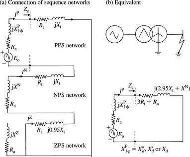
Thus, the external impedance is given by ![]() . Thus, Re = 3 × 0.00334 + 0.002 = 0.01202 pu and Xe = 2.95 × 0.2 + 0.195 = 0.785 pu. The short-circuit time constants can be calculated using Equations (5.38b) and (5.38c). However, we will use Equations (5.39a) and (5.39b) because the armature resistance and external resistance are very small in comparison with the machine’s reactances and external reactance. Thus
. Thus, Re = 3 × 0.00334 + 0.002 = 0.01202 pu and Xe = 2.95 × 0.2 + 0.195 = 0.785 pu. The short-circuit time constants can be calculated using Equations (5.38b) and (5.38c). However, we will use Equations (5.39a) and (5.39b) because the armature resistance and external resistance are very small in comparison with the machine’s reactances and external reactance. Thus
From Equation (5.38e), we have
The rms and dc fault currents are calculated using Equation (5.40b),

The rms fault current at t = 0, 10 and 100 ms is equal to 3.07, 3.02 and 2.81 pu, respectively. The dc fault current at t = 0, 10 and 100 ms is equal to 4.35, 4.16 and 2.77 pu, respectively.
5.5 Determination of synchronous machines parameters from measurements
Although calculations of machine parameters are made by machine manufacturers at the design stage, factory or field tests are generally carried out on the built machine. These are to identify the machine parameters and confirm that they are within the guaranteed or declared design values which are typically ±10% or as agreed between the manufacturer and the customer. The reactances and time constants of the machine are determined from measurements as defined in IEC and IEEE standards.
5.5.1 Measurement of positive sequence reactances, positive sequence resistance and d-axis short-circuit time constants
Measurement and separation of ac and dc current components
Several parameters can be calculated from measurements of the stator short-circuit currents during a sudden three-phase short circuit at the machine terminals. These are the positive sequence or the d-axis subtransient, transient and steady state reactances, and the d-axis short-circuit subtransient, transient and armature (dc) time constants. The machine is on open circuit and running at rated speed just before the application of the simultaneous three-phase short-circuit fault. The unsaturated reactances and time constants are determined by performing tests at a few low values of prefault stator voltage, e.g. 0.1–0.4 pu. The saturated reactances are determined from tests at rated 1 pu prefault stator voltage. Oscillograms of the three-phase short-circuit currents are taken. Recalling Equation (5.40a).
Equation (5.75a) represents the envelope of the ac rms component of the short-circuit current where
To illustrate the process of determining the machine d-axis parameters, Figure 5.15(a) illustrates the measured phase r asymmetrical current. The first step is to separate the dc and ac components of the measured current. The dc component can be calculated as the algebraic half sum of the ordinates of the upper and lower envelopes of the current whereas the ac components can be similarly determined from the algebraic half difference of the upper and lower envelopes. In practice, experience shows that this manual process is dependent on the engineer doing the analysis and can be subject to some error whereas the use of numerical filters is both more accurate and consistent. The outcome of separating the ac and dc components of the short-circuit current is illustrated in Figure 5.15(b) and the dc component alone is shown in Figure 5.15(c).
The dc (armature) time constant
As a decaying exponential, the magnitude of the dc component drops from its initial value at t = 0 to 1/e = 0.36788 of the initial value at t = Ta(3φ) where Ta(3φ) is the dc or stator or armature time constant. Ta(3φ) is indicated in Figure 5.15(c).
Steady state d-axis reactance
The peak envelope of the ac short-circuit current is shown in Figure 5.16(a). One method of determining the steady state reactance is from the oscillogram’s current value after a sufficient time so that the transient current component has completely decayed or vanished. Therefore, with ![]() read from Figure 5.16(a), we have
read from Figure 5.16(a), we have

Figure 5.16 Measured ac current component plotted on linear and logarithmic scales: (a) peak ac current envelope and components and (b) time constants from current envelopes
An alternative method that is usually used by machine manufacturers is to calculate Xd from the ratio of the field current at rated short-circuit stator current to the air-gap field current at rated open-circuit stator voltage.
Transient reactance and transient short-circuit time constant
Using Figure 5.16(a), the machine current attributable to the transient reactance is determined from the transient envelope of the ac current after subtracting the steady state current value then the transient current result is plotted on linear-logarithmic coordinates as shown in Figure 5.16(b). The envelope of the transient current component is given by
When this component is extrapolated back to zero time, it cuts the ordinate axis at ![]() and this is read from the ordinate. Therefore, the transient current is calculated as follows:
and this is read from the ordinate. Therefore, the transient current is calculated as follows:
The transient reactance can now be calculated as
The transient time constant is the time required for the transient current component to drop to 1/e = 0.36788 of its initial value as illustrated in Figure 5.16(b).
Subtransient reactance and subtransient short-circuit time constant
The machine current attributable to the subtransient reactance is determined from the upper envelope of the ac current after subtracting the transient current value. The subtransient current component is then plotted on linear-logarithmic coordinates as shown in Figure 5.16(b). The envelope of the subtransient current component is given by
When this component is extrapolated back to zero time, it cuts the ordinate axis at ![]() and this is read from the ordinate. Therefore, the subtransient current is calculated as follows:
and this is read from the ordinate. Therefore, the subtransient current is calculated as follows:
The subtransient reactance can now be calculated as
The subtransient time constant is the time required for the subtransient current component to drop to 1/e = 0.36788 of its initial value as illustrated in Figure 5.16(b).
Transient reactance at the end of the subtransient period t = 5T″d
The transient current component at the end of the subtransient period at t = 5T″d is given by ![]() and this is read from the ordinate of Figure 5.16(b). Therefore, the transient current at t = 5T″d is given by
and this is read from the ordinate of Figure 5.16(b). Therefore, the transient current at t = 5T″d is given by
Alternatively, Equation (5.37b) can be used to calculate X′d(t = 5T″d).
The reactances and short-circuit time constants measured are usually the unsaturated values. Also, since the currents in three phases are measured, the above calculations are made for each phase and an average value of each parameter is taken.
5.5.2 Measurement of NPS impedance
The NPS reactance and resistance can be determined using one of two test methods. The first is by applying a solid two-phase sustained short circuit on any two phases when the machine is running at rated synchronous speed as illustrated in Figure 5.17(a). The short-circuit current I(A), the voltage between the short-circuited phases and the healthy phase, VDiff(V), and the electric input power P3φ(W) are measured. Using Equations (2.48a) to (2.48d) with ZF = 0, it can be shown that the NPS impedance, reactance and resistance are given by
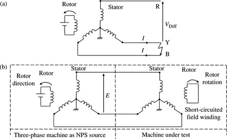
Figure 5.17 Measurement of synchronous machine NPS resistance and reactance: (a) sustained solid two-phase short-circuit and (b) three-phase NPS voltage source test
The second test method is illustrated in Figure 5.17(b). It involves applying a three-phase voltage source having a NPS phase rotation RBY to the machine being tested with the machine running at rated speed in a PPS rotation RYB and its field winding short circuited, i.e. zero internal EMF. The reason for short-circuiting the field winding is that XN, like X′d and X″d, is due to induced currents in the rotor and these currents must be able to flow unhindered. The slip of the machine being tested is therefore 200% and large double-frequency currents are induced in the damper windings. Because the NPS reactance is quite low, the applied test voltage must be very low, e.g. 0.02–0.2 pu, so as to avoid overheating. The current I(A), the applied phase voltage E(V), and the electric input power P(W) are measured. The NPS reactance and resistance are given by
The results obtained from calculations from the three phases are averaged.
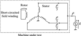
5.5.3 Measurement of zero sequence impedance
The zero sequence reactance and resistance can be determined using one of two test methods. In the first, a solid two-phase to earth sustained short-circuit fault is applied with the machine initially running at rated speed and a very low stator voltage to avoid rotor overheating or vibration. The voltage to neutral (V) on the open healthy phase and the earth (neutral) current (A) are measured. It can be shown that, using Equations (2.57a) and (2.57b) with ZF = 0, that the ZPS reactance can be calculated by dividing the measured voltage by the current.
The second test method is illustrated in Figure 5.18. It involves applying a single-phase voltage source to the machine being tested at the point where the three stator windings terminals are joined together. As for the NPS impedance test, the machine is running at rated speed and its field winding is short-circuited. The source current IZ(A), the applied source voltage E(V), and the total electric input power P(W) are measured. The ZPS reactance and resistance are given by
5.5.4 Example
Example 5.4
Consider a 50 Hz three-phase synchronous generator having rated apparent power of 165 MVA, rated power of 132 MW and rated terminal voltage of 15 kV. The results below are obtained from various tests and measurements on the generator. The armature dc resistance is 0.2% on rated voltage and rated MVA:
1. Direct axis synchronous reactance
Unsaturated or air-gap field current at rated open-circuit terminal voltage is 682 A. The field current at rated armature (stator) current on three-phase terminal short-circuit is 1418 A.
2. Sudden three-phase short-circuit test at rated synchronous speed
Figure 5.19 shows the results of the phase R current envelopes (peaks) plotted on a semi-logarithmic scale.

Figure 5.19 Measured short-circuit current envelopes plotted on semi-logarithmic scale: (a) subtransient and transient components and (b) subtransient component
A phase-to-phase sustained short-circuit test at the generator terminals gave the following results:

A two-phase to earth sustained short-circuit test at the generator terminals gave the following results:

Direct axis synchronous reactance
Alternatively, using Id = 623 A from the sudden three-phase short-circuit test, we have

Direct axis transient reactance and time constant
From Figure 5.19(a), we have
At t = T′d, the transient current component is 1/e times the initial value of 5655.4 A, i.e. 2080.5 A. Thus, the transient time constant is found from Figure 5.19 as T′d = 1.1 s.
Direct axis subtransient reactance and time constant
From Figure 5.19b, we have
At t = T″d, the subtransient current component is 1/e times the initial value of 3010.9 A, i.e. 1107.6 A. Thus, the subtransient time constant is found from Figure 5.19(b) as T″d = 39 ms.
Transient reactance at the end of the subtransient period
The transient current component at the end of the subtransient period, i.e. at t = 5T″d = 195 ms is given by ![]() A giving I′d(t = 200 ms) = 3953 A. Therefore
A giving I′d(t = 200 ms) = 3953 A. Therefore
Alternatively, using Equation (5.37b), we obtain
Usually, similar analysis is carried out for the other two phases and an average is taken. The above test results were made at 20% rated voltage. The same tests may also be carried out at other voltages.

Using the first set of results, the NPS impedance, reactance and resistance are calculated as follows:
Similar calculations are carried out using the other test results and these will give broadly similar results. The NPS impedance/reactance is then plotted against the short-circuit current and extrapolated to ![]() . The NPS reactance value should be 19%.
. The NPS reactance value should be 19%.
Using the first set of results, the ZPS reactance is calculated as follows:
Similar calculations are carried out using the other test results and these will give broadly similar results. The ZPS reactance is then plotted against the short-circuit current and extrapolated to 3 × IRated = 19053 A. This value should be 9.5%.
Using the measured PPS, NPS and ZPS reactances, and the known armature dc resistance, the armature dc time constants for various short-circuit faults are calculated as follows:
5.6 Modelling of induction motors in the phase frame of reference
5.6.1 General
For over a century, induction motors have been the workhorses of the electric energy industry. These motors are used to drive a variety of mechanical loads, e.g. fans, blowers, centrifugal pumps, hoists, conveyors, boring mills and textile machinery. The modelling of induction motors and the analysis of their short-circuit current contribution is recognised as critically important and is fully taken into account in industrial power systems, e.g. petrochemical plant, oil refineries, offshore oil platforms and power station auxiliary systems. The important characteristic in such installations is the concentrated large number of induction motors used which are clearly identifiable in terms of size, rating, location in the industrial network and, generally, electrical parameters.
Three-phase and single-phase motors are also used in some commercial installations with the latter being utilised in some domestic appliances. These motors can form an important part of the general power system load ‘seen’ at distribution network substations. The importance of the short-circuit contribution from such a cumulative motor load has only recently been recognised but, unfortunately, there is no international consensus regarding its treatment. This aspect is discussed in Chapter 7.
5.6.2 Overview of induction motor modelling in the phase frame of reference
Similar to a synchronous machine, the stator of an induction machine consists of a set of three-phase stator windings which may be star or delta connected. The rotor may be of a wound rotor or a squirrel-cage rotor construction with conducting bars placed in slots on the rotor surface. In squirrel-cage motors, the bars are short-circuited at both ends by end rings.
Due to the absence of slip rings or brushes, squirrel-cage induction motors are most rugged and are virtually maintenance-free machines. For some applications where high starting torques are required, e.g. boring mills, conveyor equipment, textile machinery, wood working equipment, etc., double squirrel-cage rotors are used. As the name implies two layers of bars are used; a high resistance one nearer the rotor surface and a low resistance one located below the first. The high resistance bars are effective at starting in order to give higher starting torque whereas the low resistance bars are effective under normal running operation.
The connection of a balanced three-phase power supply to the stator produces a MMF that rotates at synchronous speed Ns = (120 × fs)/Np where Ns is in rpm, fs is supply frequency and Np is the number of poles. This MMF induces voltages in the rotor windings and because these are short-circuited, rotor currents flow. The interaction of the rotor currents and the stator MMF produces a torque that acts to accelerate the rotor in the same direction of rotation of the stator MMF. The frequency of the rotor currents is determined by the relative motion of the stator MMF and rotor speed and is equal to Ns-Nr where Nr is the rotor speed. The relative speed, of the rotor, called slip speed, in per unit of the synchronous speed, is given by
Clearly, when the rotor is stationary, e.g. at starting, Nr = 0 and the slip s = 1.
Equation (5.83a) can be written in terms of stator MMF and rotor angular speeds ωs and ωr, in electrical radians per second, as follows:
As for synchronous machines, one of our objectives is to gain an insight into the meaning of the induction motor parameters required for use in short-circuit analysis. Prior to the derivation of the motor equations in the ryb phase frame of reference, we note that even for a squirrel-cage rotor, the rotor can be represented as a set of three-phase windings. This is because induced currents in them produce a MMF with the same number of poles as that produced by the stator windings. Also, the rotor is symmetrical as the air gap is uniform. This means that only the mutual inductances between stator and rotor windings are dependent on rotor angle position. Figure 5.20 illustrates the stator and rotor circuits of an induction motor.

Assuming that the axis of phase r rotor winding leads that of phase r stator winding by θr where
Using Equation (5.83c), we can write
Initially, we consider the rotor to have a single rotor winding to correspond to that of wound rotor or a single squirrel-cage rotor. The time domain stator and rotor voltage equations, with (s) and (r) denoting stator and rotor, respectively, can be written in matrix form as
where e, i and ψ are 3 × 1 column matrices and Rs and Rr are 3 × 3 diagonal matrices of Rs and Rr elements, respectively. Rs and Rr are stator and rotor resistances, respectively.
The time domain stator and rotor flux linkage equations for a magnetically linear system are given by
 (5.86b)
 (5.86c)
Lσs and Lms are the leakage and magnetising inductances of the stator windings, Lσr and Lmr are the leakage and magnetising inductances of the rotor windings and Lsr is the amplitude of the mutual inductance between the stator and rotor windings. The magnetising and mutual inductances are associated with the same magnetic flux paths, hence Lms, Lmr and Lsr are related by the stator/rotor turns ratio as follows:
where the prime denotes rotor quantities that are referred to the stator. Thus
 (5.87b)
 (5.87c)
Substituting Equation (5.87d) into Equation (5.85), we obtain
We have used p instead of s since the latter is used to denote slip speed.
5.7 Modelling of induction motors in the dq frame of reference
5.7.1 Transformation to dq axes
The next step is to transform the stator and rotor quantities to the d and q axes reference frame. However, because we are concerned in this book with short circuit rather than electromechanical analysis, we will fix our reference frame to the rotor as in the case of synchronous machines. This introduces an advantage that will become apparent later. The d-axis is chosen to coincide with stator phase r axis at t = 0 and the q-axis leads the d-axis by 90° in the direction of rotation. Therefore, the stator and rotor quantities can be transformed using the transformation matrix given in Equation (5.7b). It can be shown that the transformation of Equations (5.87d) and (5.87e) gives
 (5.88a)
 (5.88b)
Because the rotor windings are short-circuited,
We note that the speed voltage terms in the rotor voltages of Equation (5.88b) are zeros because of our choice of reference frame for the rotor quantities to coincide with the rotor rather than with the synchronously rotating MMF.
The above equations are in physical units. However, it can be easily shown that they take the same form in per unit because the stator rated quantities are taken as base quantities. The d and q axes transient equivalent circuits are obtained by substituting Equation (5.88a) into Equation (5.88b). The result is the operational equivalent circuit shown in Figure 5.21(a) that is identical in both the d and q axes because of the symmetrical structure of the rotor. The steady state equivalent circuit, shown in Figure 5.21(b), is derived by converting the time variables into phasors and setting all derivatives to zero. We note that in order to simplify the notation, we have dropped the prime from the rotor resistance and inductance parameters.

5.7.2 Complex form of induction motor equations
To simplify the mathematics, we can replace all the voltage and flux linkage equations for the d and q axes of Equations (5.88a) and (5.88b) by half the number of equations if we define new complex variables Vs, Is, It, ψs, ψr such that
Therefore, combining the fluxes and voltages from Equations (5.88a) and (5.88b) according to Equation (5.89), we obtain
5.7.3 Operator reactance and parameters of a single-winding rotor
In order to gain an understanding of the origin and meaning of the various motor parameters, e.g. transient reactance and time constant, we will use the method of operator axis reactance analysis for the simplicity and clear insight it provides. Since the motor operational equivalent circuit of Figure 5.21(a) is identical for both the d and q axes, the d and q axes operator reactances will be identical. By substituting Equation (5.91b) for ψr into Equation (5.90b), we obtain
which when substituted into Equation (5.91a) for ψs and simplifying, we obtain
It can be shown that after further manipulation, Equation (5.92a) can be written as
 (5.93b)
T′o and T′ are the motor’s open-circuit and short-circuit transient time constants, respectively. As for the synchronous machine, to obtain the time constants in seconds, the per-unit time constants of Equations (5.93a) and (5.93b) should be divided by ωs = 2πfs where fs is the system power frequency. The motor operational reactance is defined as X(p) = ωsψs/Is, hence, from Equation (5.92b), we obtai
The effective motor reactance at the instant of an external disturbance is defined as the transient reactance X′. Using Equation (5.94a), this is given b
This can also be expressed in terms of the electrical parameters of the stator and rotor circuits using Equations (5.93a) and (5.93b) as follows:
5.7.4 Operator reactance and parameters of double-cage or deep-bar rotor
Many induction motors are designed with a double squirrel-cage rotor. Also, many large MW size motors have deep-bar cage windings on the rotor designed to limit starting currents. For both double-cage and deep-bar rotors, we assume that the end-rings resistance and the part of the leakage flux which links the two rotor windings, but not the stator, are neglected. Therefore, we represent both rotor types by two parallel rotor circuits as shown in the operational equivalent circuit of Figure 5.22(a). The corresponding steady state equivalent circuit is shown in Figure 5.22(b). Figure 5.22(c) shows an alternative steady state equivalent circuit where the two rotor branches are converted into a single equivalent branch whose resistance and reactance are functions of motor slip s as follows:
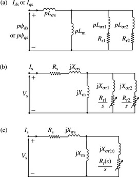
Figure 5.22 Equivalent circuits of an induction motor with a double squirrel-cage or deep-bar rotor: (a) operational equivalent circuit, (b) steady state equivalent circuit and (c) circuit (b) with a single equivalent rotor branch
 (5.95b)
From the operational circuit of Figure 5.22(a), and as in the case of a single rotor winding, the complex form of the motor voltage and flux linkage equations can be written by inspection as follows:
The derivation of the operational reactance is similar to that in the case of a single rotor winding except that more algebra is involved. The steps are summarised as follows: substitute Equation (5.97b) in Equation (5.96b), Equation (5.97c) in Equation (5.96c), eliminate Is and express Ir1 in terms of Ir2, express Ir1 and Ir2 in terms of Is and substitute these results back in Equation (5.97a). It can be shown that the result is given by
 (5.98a)
Using X(p) = ωsψs/Is, the motor operational reactance can be written as
 (5.98b)
As in the case of synchronous machines, in order to derive the electrical parameters of the motor, it can be shown that Equation (5.98b) can be rewritten as
 (5.100b)
 (5.100c)
Again, as in the case of synchronous machines, we make use of an approximation that reflects practical double squirrel-cage rotor or deep-bar rotor designs. The winding resistance of the lower cage winding Rr1 is much smaller than Rr2 of the second cage winding nearer the rotor surface. This means that T2 (and T3) is much smaller than T1, and T5 (and T6) is much smaller than T4. Therefore, Equation (5.99) can be expressed in terms of factors as follows:
are the open-circuit transient and subtransient time constants, and
are the short-circuit transient and subtransient time constants.
The effective motor reactance at the instant of an external disturbance is defined as the subtransient reactance X″. Using Equation (5.101), this is given by
which, using Equations (5.100) and (5.102), can be written in terms of the motor reactance parameters as follows:
As in the case of synchronous machines, the second rotor cage is no longer effective at the end of the subtransient period and the beginning of the transient period. Thus, using Equation (5.95) previously derived for the single rotor cage, we have
Using Equation (5.104) for X′ in Equation (5.103a) for X″, we obtain the following useful relationship between the subtransient and transient reactances and time constants
In order to determine the motor reactance under steady state conditions, we recall that the rotor slip is equal to s and thus the angular frequency of the dq axes stator currents is sωs. Therefore, the steady state motor impedance can be determined by putting p = jsωs in X(p) expression given in Equation (5.101).
We can express the induction machine operational reactance given in Equation (5.101) as a sum of partial fractions as follows:
which, using Equations (5.103a) for X″ and (5.104) for X′, can be written as
5.8 Induction motor behaviour under short-circuit faults and modelling in the sequence reference frame
The most common types of short-circuit faults studied in power systems are the balanced three-phase and unbalanced single-phase to earth faults. Having derived the motor reactances and time constants, we are now able to proceed with analysing the behaviour of the motor under such fault conditions.
5.8.1 Three-phase short-circuit faults
Armature (stator) short-circuit time constant
Using X(p) = ωsψs/Is in Equation (5.96a), the stator current is given by
 (5.107)
As for synchronous machines, we can make an assumption in the term ωsRs/X(p) to neglect the rotor resistances in the factors of X(p) given in Equation (5.101). This is equivalent to setting infinite rotor time constants or neglecting the decay in the corresponding short-circuit currents. Mathematically speaking, this is equivalent to setting p → ∞ in Equation (5.94a) and Equation (5.101). Thus, using Equation (5.94a) for a single rotor winding, we obtain X(p) = X′ giving
Also, using Equation (5.101) for a double squirrel-cage or deep-bar rotor, we obtain X(p) = X″ giving
Therefore, the armature or stator time constant Ta is defined as follows:
 (5.108)
Total short-circuit current contribution from a motor on no load
Unlike a synchronous machine, since the induction motor has no rotor excitation, it draws its magnetising current from the supply network whatever the motor loading is, i.e. from no load to full load operation. Therefore, the motor cannot be operated open-circuited in a steady state condition! Prior to the short-circuit fault, the motor is assumed connected to a balanced three-phase supply and operating at rated terminal voltage. To simplify the mathematics, we assume that the motor is running at no load and hence the slip is very small and nearly equal to zero. Let the real instantaneous voltage, complex instantaneous voltage and complex phasor voltage values of the phase r stator voltage, just before the short-circuit, be given by
where θo is the initial phase angle that defines the instant of fault on the phase r voltage waveform at t = 0. Neglecting stator resistance, i.e. letting Rs = 0, using Equation (5.83c) and putting p = 0 in Equation (5.107), we obtain
Using Equation (5.101), X(p = 0) = Xσs + Xm and using Equation (5.109c), the stator steady state current phasor is given b
Equation (5.110a) shows that the current lags the voltage by 90°, as expected.
Using the superposition principle, the total motor current after the application of the short circuit is the sum of the initial steady state current and the change in motor current due to the short circuit. The latter is obtained by applying a voltage source at the point of fault equal to but out of phase with the prefault voltage, i.e. ![]() . Since the Laplace transform of δVs is equal to
. Since the Laplace transform of δVs is equal to
we obtain from Equation (5.107)
Substituting the partial fractions Equation (5.106) for X(p), we obtain
 (5.111b)
The complex instantaneous current δIs(t) is obtained by taking the inverse Laplace transform of Equation (5.111b). The total short-circuit current Is(total)(t) is the sum of the prefault current given in Equation (5.110a) and δIs(t). The real instantaneous phase r stator short-circuit current is given by ![]() . For all practical purposes, 1/Ta, 1/T′, and 1/T″ are negligible in comparison with ωs and ωr. Therefore, and after much mathematical operations, it can be shown that the total phase r short-circuit current is given by
. For all practical purposes, 1/Ta, 1/T′, and 1/T″ are negligible in comparison with ωs and ωr. Therefore, and after much mathematical operations, it can be shown that the total phase r short-circuit current is given by
 (5.112a)
The first term is the ac component that consists of a subtransient and a transient component which decay with time constants T′ and T″, respectively. The second term is the dc component that has an initial magnitude that depends on θo and it decays with a time constant Ta. Unlike a synchronous machine, there is no steady state ac component term and hence the short-circuit current decays to zero. The frequency of the short-circuit current is slightly lower than the power frequency by the factor (1 - s).
For a single cage/winding rotor, it can be shown that the instantaneous current is given by
 (5.112b)
In this case, the current consists of only one ac component and a dc component.
The phases y and b currents are obtained by replacing θo with θo - 2π/3 and θo + 2π/3 respectively.
Figure 5.23 shows typical short-circuit current waveforms of a large 6.6 kV 4700 hp motor with a deep-bar rotor having the following parameters: X″ = 0.16 pu, X′ = 0.2 pu, X = Xσs + Xm = 3.729 pu and Rs = 0.0074 pu.

Simplified motor short-circuit current equations
For practical applications, further simplifications in the short-circuits current equations can be made. The motor slip s is typically less than 1% for large motors and less than 4–5% for smaller motors. Therefore, if (1 - s) is replaced by 1, then the peak current envelope at any time instant, for a double-cage or deep-bar rotor, assuming maximum dc offset, is given by
For a single cage/winding rotor, the peak current envelope is given by
Motor current change due to the short-circuit fault
In the above analysis, we determined the total motor current under a three-phase short-circuit at the motor terminals when the motor is running on no load. This current consisted of the steady state current just before the fault and the current change due to the short circuit. For some practical analysis, it is useful to calculate the current change only and account differently for the motor initial loading conditions. From Equations (5.113a) and (5.115a), we can show that the equations that give the current change for a double-cage and a single-cage rotor are given by
Positive sequence reactance and resistance
From Equation (5.112a) for a double-cage or deep-bar rotor, the instantaneous current change due to the short-circuit fault is obtained by ignoring the prefault current ![]() . Thus with 1 - s ≈ 1, we can express the instantaneous power frequency component of the short-circuit current as ir(t) = Real[Ir(t)] where Ir(t) is phase r complex instantaneous current given by
. Thus with 1 - s ≈ 1, we can express the instantaneous power frequency component of the short-circuit current as ir(t) = Real[Ir(t)] where Ir(t) is phase r complex instantaneous current given by
is the equivalent time-dependent motor PPS reactance. In the case of a single-winding rotor, using Equation (5.112b), the time-dependent motor PPS reactance is given by
From Equation (5.119b) for a motor with a double-cage or deep-bar rotor, Xp = X″ at t = 0 or the instant of short-circuit, and Xp = X′ at t = 0 with the subtransient current component neglected. At the end of the subtransient period, i.e. at t ≈ 5T″, then from Equation (5.119b), we obtain
The effective motor steady state PPS reactance is infinite because the motor does not supply a steady state short-circuit current. From Equation (5.119c) for a single winding rotor, Xp = X′ at the instant of short-circuit and is infinite in the steady state.
The complex instantaneous PPS current is given by
Figure 5.24 shows the PPS motor equivalent circuits for a three-phase short-circuit at the motor terminals.

Figure 5.24 Induction motor PPS equivalent circuits for a three-phase short circuit at its terminals: (a) transient PPS time-dependent equivalent circuit and (b) PPS fixed impedance equivalent circuits at various time instants
The PPS impedance, Zp = Rp + jXp, at the instant of short-circuit fault can also be derived from the motor steady state equivalent circuit. For example, for a single winding rotor shown in Figure 5.21(b), Zp is the impedance that would be seen at the motor terminals at starting (i.e. when s = 1). Thus, it can be shown that the PPS resistance and PPS reactance are given by
The term R2r is negligible in comparison with either of the two terms Xr(Xm + Xσr) or (Xm + Xσr)2, thus, Xp and Rp reduce to
Although unnecessary, further simplification in Rp and Xp can be made if we consider that 2Xσr/Xm « 1 to obtain Rp = Rs + Rr and Xp = Xs + Xσr.
Effect of short-circuit fault through an external impedance
The effect of external impedance (Re + jXe) on the current change can be considered in the same manner as for synchronous machines. For the double-cage or deep-bar rotor, the peak current envelop and time constant equations are given by
 (5.121a)
 (5.121b)
 (5.121c)
Where the stator and external resistances are much smaller than the reactances, the transient and subtransient time constants reduce to
For a single-cage rotor, the corresponding equations are given by
where T′e is as given in Equation (5.121c) or Equation (5.121e), and
5.8.2 Unbalanced single-phase to earth short-circuit faults
Short-circuit current equations
Consider an induction motor with a star-connected solidly earthed stator winding. When a loaded induction motor is subjected to an unbalanced single-phase short circuit at its terminals, the faulted phase will initially supply a short-circuit current.
However, under such a fault condition, there is an interaction between the motor and other short-circuit current sources in the network, e.g. synchronous machines through the ZPS network. The current contribution will therefore be affected by other sources in the network. Further, the phase current contribution would not decay to zero as in the case of a three-phase fault because the other two healthy phases remain supplied from the network and continue to provide some excitation which maintain some flux. Although the PPS current contribution will decay to zero, the NPS current contribution will not so long as the single-phase fault condition continues to exist. In Section 5.8.4, we describe a sudden short-circuit test immediately after motor disconnection from the supply network. It can be shown that the change in motor current supplied under a single-phase fault at the motor terminals, in the case of a double-cage or a deep-bar rotor, expressed in terms of the peak current envelope, is given by
 (5.122a)
 (5.122b)
where T′(1φ) is as given in Equation (5.122b) and
Negative sequence reactance and resistance
As for a synchronous machine, the NPS reactance of the induction motor XN does not vary with time. XN = X″ for a double-cage or deep-bar rotor and XN = X′ for a single-cage rotor. In addition, the NPS impedance, ZN = RN + jXN, can be derived from the motor steady state equivalent circuit shown in Figure 5.21(b) for a single-cage rotor and Figure 5.22(b) for a double-cage or deep-bar rotor. We recall that under a three-phase PPS excitation, both the stator MMF and the rotor rotate in the same direction. However, under three-phase NPS excitation, the NPS stator currents will produce a MMF that rotates in the opposite direction to the rotor. Using Equation (5.83a), the motor’s NPS slip can be calculated as follows:
i.e. in the motor NPS equivalent circuit, s should be replaced by (2 – s). For large motors, s is typically less than around 1% and even for small motors, s is less than around 4% or 5%. Therefore, if we replace s with (2 – s) = 2 in Figure 5.21(b), we can calculate the motor NPS resistance and NPS reactance, as follows:
As in the case of PPS impedance, the term R2r is negligible and can be neglected. Therefore, Equation (5.124b) reduces to
Further approximation in RN can be made if we assume that 2Xσr/Xm « 1 giving
This produces an error in RN of typically a couple of per cent only.
Zero sequence reactance and resistance
The ZPS impedance of an induction motor is infinite if the stator winding is either delta connected, or star connected with the neutral isolated. For a star-connected winding with an earthed neutral, then as for a synchronous machine, the ZPS reactance XZ is finite, being smaller than the motor starting reactance (subtransient or transient as appropriate to the rotor construction) and does not vary with time. The ZPS resistance can be assumed equal to the stator ac resistance.
5.8.3 Modelling the effect of initial motor loading
When the motor is loaded, it draws active and reactive power from the supply network. Using the motor transient and subtransient reactances for a double-cage rotor or transient reactance for a single-cage rotor, the motor internal voltages behind subtransient and transient reactances, E′m and E″m, are given by
Equations (5.125) are illustrated in Figure 5.25.

Figure 5.25 Representation of initial motor loading before the short-circuit fault: (a) motor internal voltage behind subtransient reactance, (b) motor internal voltage behind transient reactance at t = 0 and (c) motor internal voltage behind transient reactance at t = 5T″
The peak short-circuit current changes in the case of a three-phase fault given in Equations (5.117a) and (5.118a) are modified as follows:
From Equation (5.125) we observe that the motor internal voltage is equal to the terminal voltage less the voltage drop across the motor subtransient or transient impedance. For a 1 pu motor terminal voltage, typical values of motor subtransient and transient reactances, and various motor loading, the internal voltage magnitude can typically vary between 0.85 and 0.95 pu. Therefore, ignoring the initial motor loading and using 1 pu instead of the actual internal voltages represents a conservative assumption. This assumption is made by the American IEEE C37.010 Standard and UK ER G7/4 Guideline. This will be discussed in detail in Chapter 7.
5.8.4 Determination of motor’s electrical parameters from tests
Steady state equivalent circuit: stator resistance test
The stator winding dc resistance of a three-phase induction motor is measured by connecting a dc voltage source across two stator terminals. No induced rotor voltage can occur under de stator excitation and hence the resistance ‘seen’ by the dc voltage source is the stator de resistance. By applying a known dc voltage and measuring the dc current, the stator de resistance can be calculated. The calculation depends on whether the stator winding is star or delta connected as shown in Figure 26.5(a) and (b) where the star is assumed to have an isolated neutral. In physical units, the stator de resistance Rs(dc) is given by

Figure 5.26 Measurement of stator de resistance of an induction motor: (a) star-connected stator winding with isolated neutral and (b) delta-connected stator winding
 (5.127)
If the test is repeated for the other two sets of terminal connections, then an average is taken. Rs(dc) has to be corrected for skin effect by multiplying it by the skin effect factor which is typically between 1.05 and 1.25.
Steady state equivalent circuit: locked rotor test
This test circuit is shown in Figure 5.27(a).

Figure 5.27 Measurement of electrical parameters of an induction motor: (a) locked rotor test and (b) no-load test
The stator is connected to a balanced three-phase ac voltage source and the rotor shaft is locked mechanically to prevent it from turning. Since the slip s = 1, the rotor impedance is several times smaller than that under rated running condition (because operating slip is typically between 0.001 and 0.05) and is typically 30–50 times smaller than the magnetising reactance. Thus, the locked rotor test is broadly analogous to a transformer short-circuit test. The test voltage applied should initially be very small and then gradually increased until rated or full load stator current is drawn. To avoid overheating, the applied voltage is significantly smaller than the rated voltage so that the motor current is limited to the rated value. If rated voltage is applied, the locked rotor current drawn is very large and is typically four to seven times the rated current value. The combination of a low-test voltage and a low rotor impedance results in a very small exciting current and hence the iron loss and magnetising branches can be neglected with an insignificant loss of accuracy. As shown in Figure 5.27(a), the equivalent motor impedance ‘seen’ from the test terminals is given by
The measured stator quantities are line-to-line voltage VLL, stator current Is, three-phase input power P3φ, and three-phase input reactive power Q3φ. For either a star or a delta-connected stator winding, the equivalent resistance and reactance of Equation (5.128) are calculated as follows:
Alternatively, using the line-to-line stator voltage instead of the reactive power
 (5.130a)
and the equivalent reactance is calculated as follows:
Using the measured stator de resistance or better still its corrected skin effect value, the rotor resistance can be calculated from Equation (5.129a) as
In Equation (5.130b), the sum of the stator and rotor leakage reactances is calculated. In the absence of manufacturer design data that provides the ratio of these reactances, the division shown in Table 5.1 for different types of motors as classified by the National Electrical Manufacturers Association (NEMA) may be used.
Table 5.1 Estimation of induction motor stator and rotor leakage reactances using NEMA motor class in the absence of design data
| NEMA Motor Design Class | Xσs in % of XEq | Xσr in % of XEq |
|---|---|---|
| Wound rotor | 50 | 50 |
| Class A | 50 | 50 |
| Class B | 40 | 60 |
| Class C | 30 | 70 |
| Class D | 50 | 50 |
If the motor design class is not known, then Xσs and Xσr may be assumed to be equal. The locked rotor test may also be carried out at reduced frequency to account for skin depth and a more accurate rotor resistance under rated operating conditions where the rotor current frequency may be between 0.5 and 2.5 Hz. IEEE Standard 112 recommends a frequency of 1/4 of the rated power frequency. In general, this method tends to provide better results for large motors above 20 hp but for small motors, the results obtained from the power frequency test are generally satisfactory.
Steady state equivalent circuit: no-load test
This test circuit is shown in Figure 5.27(b). The stator winding is connected to a three-phase source supplying rated voltage and frequency and the motor is run without shaft load. As a result, the rotor will rotate at almost synchronous speed, i.e. slip speed s ≈ 0. Thus, Rr/s → ∞ and the motor equivalent circuit is broadly similar to that of a transformer on open-circuit. Therefore, the rotor impedance branch is effectively open-circuit and the current drawn by the stator is fully attributed to the exciting current. The stator quantities measured are; line-to-line voltage VLL, current Is, three-phase input power P3(φ) and three-phase input reactive power Q3φ. The iron loss resistance associated with the magnetising impedance can be calculated, if required, by connecting this resistance in parallel with the magnetising reactance. Using the inequality Rm/Xm » 1, the motor equivalent impedance as seen from the test terminals is approximately given by
The measured input power includes rotational losses (friction and windage, iron and stray load losses) as well as stator copper losses and is given by
Using the measured input reactive power, we have
Using the measured input reactive power and stator current, and the calculated value of Xσs, Xm is calculated using Equation (5.131c). Also, Rm is calculated from Equation (5.131b) using the measured input power and stator current, as well as the calculated quantities Rs and Xm. If the friction/windage and stray losses are not known, then they may be neglected with little error. If required, the very small stator copper losses in Equation (5.131b) may also be neglected and the calculation of Rm and Xm proceeds similarly.
Transient parameters from a sudden three-phase short-circuit immediately after motor disconnection
This method consists of two steps; the first is to disconnect the motor from the supply network and the second is to quickly apply a simultaneous three-phase short-circuit fault at the motor terminals. As for synchronous machines, this is usually a suitable test method for the determination of the motor subtransient and transient parameters.
Immediately upon supply disconnection, the flux linking the closed rotor inductive circuits prevents the rotor current from changing instantaneously to zero. This flux will decay in a manner determined by the rotor open-circuit subtransient and transient time constants T″o and T′o, respectively. It can be shown that the phase r open-circuit motor terminal voltage following motor disconnection, where the motor has a double squirrel-cage or deep-bar rotor, is given by
where Irms is the initial stator current before motor disconnection and δ is its phase angle.
The three-phase short circuit is applied a few cycles after the removal of the motor supply. The range of values of T″o, even for large induction motors, tends to be between a few ms to about 30 ms so that the voltage component associated with T″o will be negligible by the time the short circuit is applied at time ts as illustrated in Figure 5.28. The only relevant component is therefore the one associated with T′o. It should be noted that this is the only component applicable in the case of a rotor with a single rotor winding, e.g. a single squirrel-cage rotor or a wound rotor. Therefore
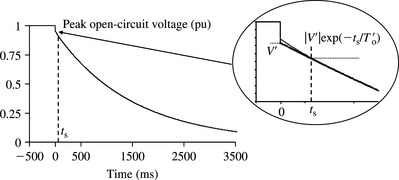
Figure 5.28 illustrates the peak envelope of the motor phase r open-circuit voltage after supply disconnection. At the instant of short-circuit t = ts, following the decay of the subtransient voltage component, the rms value of the motor open-circuit voltage is given by
This voltage can be measured from the recorded voltage envelope. Since the motor is on open circuit, the equations that describe the motor short-circuit currents will be the same as those derived in Equations (5.117a) and (5.118a) or (5.122a) and (5.123a) but with Vrms replaced with the magnitude of Voc of Equation (5.133). The envelope of the current can be used to determine the motor subtransient and transient reactances and time constants as described for synchronous machines.
5.8.5 Examples
Example 5.5
A 50 Hz three-phase induction motor of a single squirrel-cage rotor construction drives a condensate pump in a power generating station and has the following data: rated phase-to-phase voltage = 3.3 kV, rated three-phase apparent power= 900 kVA, Rs = 0.0968 ω, Xσs = 1.331 ω, Xm = 38.7 ω, and Rr = 0.0726 ω, Xσr = 0.847 ω at rated slip. The rotor parameters referred to the stator voltage base. Calculate the motor parameters in pu on kVA rating, the motor transient reactance, open circuit, short circuit and armature time constants.
Base voltage and base apparent power are 3.3 kV and 0.9 MVA, respectively. Base impedance is equal to (3.3)2/0.9 = 12.1 Ω. Therefore, Rs = 0.0968/12.1 = 0.008 pu, Xσs = 1.331/12.1 = 0.11 pu, Xm = 38.7/12.1 = 3.2 pu, Rr = 0.0726/12.1 = 0.006 pu, Xσr = 0.847/12.1 = 0.07 pu.
From Equations (5.108)
From Equations (5.93) and (5.95b)
In many situations, the internal motor parameters may not be known but T′ and X′ may be known from measurements. In this case, the following empirical formula for T′ that provides sufficient accuracy may be used T′ = X′/ωsRr. This is equivalent to replacing the numerator of Equation (5.93b) by X′. The numerator of Equation (5.93b) is equal to 0.1763 pu and hence the use of T′ = X′/ωsRr to calculate the transient time constant gives a slightly higher and thus conservative time constant by about 1.2%.
Example 5.6
In the system shown in figure in Example 5.6, the two induction motors are identical and have the data given in Example 5.5.
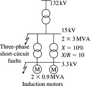
Calculate the peak short-circuit current contribution of the motors at t = 0, 10 and 100 ms for a three-phase short-circuit fault at (a) the 3.3 kV terminals of the motors, and (b) the 15 kV medium voltage busbar. Assume a 1 pu initial voltage at the 3.3 and 15 kV busbars and that the motors are initially unloaded. Consider only the change in motor current due to the fault.
(a) Three-phase short-circuit fault at the motor 3.3 kV busbar terminals
Using Equation (5.118a), the rms and dc short-circuit currents from each motor are equal to
The rms current at t = 0, 10 and 100 ms is equal to 5.6, 5.03 and 1.92 pu, respectively. The dc current at t = 0, 10 and 100 ms is equal to 7.92, 6.88 and 1.94 pu, respectively. The peak current contribution at t = 0, 10 and 100 ms is equal to 15.84, 13.76 and 3.88 pu respectively. The total current contribution from both motors at t = 0, 10 and 100 ms is equal to 31.68, 27.52 and 7.76 pu, respectively.
(b) Three-phase short-circuit fault at the 15 kV medium voltage busbar
The equivalent transient reactance of the two motors is 0.1785/2 = 0.08925 pu. The external impedance is equal to the transformer’s impedance and is calculated on 0.9 MVA base as
The time constants of the equivalent motor representing the two parallel motors do not change but the stator resistance and transient reactance are halved so that Rs = 0.004 pu and X′ = 0.08925 pu. The external impedance modifies the motor’s short-circuit time constant according to Equation (5.121e), thus
where X = (3.2 + 0.11)/2 = 1.655 pu.
The armature time constant is modified using Equation (5.121g) to
Using Equation (5.121f), the rms and dc short-circuit currents are given by
The rms current at t = 0, 10 and 100 ms is equal to 8.386, 7.73 and 3.7 pu, respectively. The dc current at t = 0, 10 and 100 ms is equal to 11.86, 9.86 and 1.87 pu, respectively. The peak current contribution at t = 0, 10 and 100 ms is equal to 23.7, 19.72 and 3.74 pu, respectively.
5.9 Modelling of wind turbine generators in short-circuit analysis
5.9.1 Types of wind turbine generator technologies
The most important feature of wind turbine generators that are directly connected to the ac network is that induction, rather than synchronous, generators are used in nearly all commercial wind turbine installations throughout the world. Synchronous generators are also widely used but, currently, these are not directly connected to the ac network. Rather, they are connected through a back-to-back power electronics converter. The use of directly connected synchronous generators may become possible if the development of variable speed gearbox technology proves sufficiently reliable and commercially attractive. The variable speed gearbox has a variable input speed on the turbine side but produces constant output synchronous speed. This technology is currently under research, development and field testing and large-scale commercial use may be imminent. The four currently most used wind turbine generator technologies in large-scale wind farm installations world wide are briefly described below.
‘Fixed’ speed induction generators
These are essentially similar to squirrel-cage induction motors and are driven by a wind turbine prime mover at a speed just above synchronous speed, normally upto 1% rated slip for today’s large wind turbines. Because the speed variation from no load to full load is very small, the term ‘fixed’ speed tends to be widely used. The generator is coupled to the wind turbine rotor via a gearbox as shown in Figure 5.29. The design and construction of the stator and rotor of an induction generator are similar to that of a large induction motor having a squirrel-cage rotor.

Small speed range wound rotor induction generators
This type of induction generator utilises a three-phase wound rotor winding that is accessible via slip rings. The rotor windings are usually connected to an external resistor circuit through a modern power electronics converter that modifies the rotor circuit resistance by injecting a variable external resistance on the rotor circuit. This method enables control of the magnitude of rotor currents and hence generator electromagnetic torque. This enables the speed of the generator to vary over a small range, typically upto 10%. Figure (5.30) illustrates this type of wind turbine generator.

Variable speed doubly fed induction generators
These are variable speed wound rotor induction generators that utilise two bidirectional back-to-back static power electronic converters of the voltage source type as shown in Figure 5.31. One converter is connected to the ac network either at the generator stator terminals or the tertiary winding of a three-winding generator step-up transformer. The other converter is connected to the rotor windings via a slip rings.

The purpose of the rotor-side converter is to inject a three-phase voltage at slip frequency onto the rotor circuit. The injected voltage can be varied in both magnitude and phase by the converter controller and this controls the rotor currents almost instantaneously. This control provides two important functions. The first is variation of generator electromagnetic torque and hence rotor speed. The second may be constant stator reactive power output control, stator power factor control or stator terminal voltage control. Typical speed control range for a modern MW class wind turbine doubly fed induction generator may be between 70% and 120% of nominal synchronous speed with the 120% usually referred to as the rated speed at which rated MW output is produced.
Variable speed series converter-connected generators
These are ac generators that are connected to the ac network through a ac/dc/ac series back-to-back converter with a rating that matches that of the generator. Many of such electrical generators presently in use are low speed multi-pole ‘ring’ type synchronous generators that are directly driven by the wind turbine rotor, i.e. there is no gearbox between the turbine rotor and generator. Other types of electrical generators are also used such as squirrel-cage induction generators but these are connected to the turbine rotor through a gearbox. In a series converter-connected generator, the full output of the generator is fed into a power electronics rectifier or a voltage sourced converter, then through a dc link into a static power electronics inverter as illustrated in Figure 5.32. In this type of technology, the electrical generator is isolated from the ac network. The generator side converter is usually used for controlling the generator speed and the network side inverter is usually used for voltage/reactive power control and dc link capacitor voltage control.

5.9.2 Modelling of fixed speed induction generators
We have already presented the modelling of synchronous generators and induction motors for short-circuit analysis. The PPS and NPS short-circuit contribution of a fixed speed induction generator can be represented in a similar way to that of an induction motor. The equations of subtransient and transient reactances and time constants derived for induction motors can also be used for induction generators. The stator windings of these generators are usually connected in delta or star with an isolated neutral. Thus, their ZPS impedance to the flow of ZPS currents is infinite.
5.9.3 Modelling of small speed range wound rotor induction generators
When a three-phase short-circuit fault occurs at the terminals of an induction generator, the generator will inherently supply a large stator short-circuit current. As we have already seen for synchronous generators and induction motors, due to the theorem of constant flux linkages, a corresponding increase in the generator’s rotor currents occurs. For a small speed range wound rotor induction generator, the rotor converter used to control the rotor currents is suddenly subjected to large overcurrents. The junction temperature of the thyristor or transistor switches used in the converter cannot be exceeded or they will be damaged. The short-term over-current capability of the electronic switches used within the converter is extremely limited and almost practically non-existent if they are normally designed to operate at or close to their rated junction temperature. Therefore, when the instantaneous current limit of the switches is exceeded, they are immediately blocked and this effectively inserts the entire external resistance in series with the rotor circuit. The blocking of the switches is very fast and occurs typically in about 1 ms. This causes, the rotor winding of the generator to become effectively similar to that of a conventional wound rotor induction motor but with an additional external resistance. Therefore, the generator’s initial short-circuit current contribution to a fault on the network can be calculated as for an induction motor with a single-winding rotor having an increased rotor resistance. Using Equation (5.100b) for T4 and Equation (5.102b) for T′ = T4, and designating the external resistance as Re, the transient time constant is given as
 (5.134)
The additional rotor resistance reduces the motor transient time constant and hence increases the rate of decay of the ac current component of the short-circuit current. Figure 5.33 illustrates the effect of external rotor resistance on the stator short-circuit rms current for a typical 2 MW induction generator.

Figure 5.33 Effect of external rotor resistance on the short-circuit current of a small speed range wound rotor induction generator
As the stator short-circuit current decays, and the rotor current drops below the protection or the converter-controlled reference value, some generator manufacturers design their converters to quickly unblock the switches and regain control of the rotor currents back to some specified value. This means that the generator starts to supply a constant low value stator short-circuit current.
5.9.4 Modelling of doubly fed induction generators
The dq model of a doubly fed induction generator with a wound rotor is similar to that of an induction motor presented in Equation (5.88). However, there is an important exception; the dq rotor voltages edr and eqr given in Equation (5.88b) are not equal to zero. They are equal to the voltages injected by the rotor-side converter. The steady state equivalent circuit of the doubly fed induction generator is shown in Figure 5.34 with all rotor quantities referred to the stator.
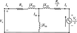
A three-phase short-circuit fault in the network will cause a symmetrical voltage dip at the generator terminals and large oscillatory currents in the rotor winding connected to the rotor-side converter. Controlling large rotor currents requires a large and uneconomic rotor voltage rating. Therefore, the large rotor currents can flow through and damage the converter switches. However, to protect these switches from damage, one method is to use a converter protective circuit called a ‘crowbar’ circuit that is connected to the rotor winding through anti-parallel thyristors as illustrated in Figure 5.31. When a large instantaneous rotor current in any phase in excess of the allowable converter limit is detected, the converter switches are immediately blocked and the thyristors of the crowbar circuit are fired to prevent a large overvoltage on the dc link. This crowbar action effectively short circuits and bypasses the converter and causes the rotor currents to flow into the crowbar circuit. Since the generator may be operating at a speed significantly above synchronous speed, some crowbar circuits may also insert an impedance, usually a resistance only, in series with the rotor winding in order to reduce the reactive power consumption of the generator and improve its electric torque/speed performance. The blocking of the converter switches and operation of the crowbar protective circuit are very fast and may occur well within 2 ms. Once the converter is bypassed, the rotor winding of the generator appears effectively similar to that of a conventional wound rotor induction generator with an external rotor resistance Rcb as shown in Figure 5.35a.
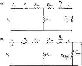
Figure 5.35 Doubly fed induction generator with operation of rotor side converter protection: (a) converter short-circuited by a crowbar through resistance Rcb and (b) converter protected by a dc chopper through resistance RChop in parallel with dc link capacitor
What happens next depends on the requirement of the power system to which the generator is connected. The whole wind turbine generator may be disconnected from the ac grid. Alternatively, only the rotor converter may be disconnected but not the wind turbine generator that continues to operate as a wound rotor induction machine with a higher rotor resistance. A more grid friendly converter control strategy is to keep the turbine generator connected to the grid and rotor converter connected to the rotor but quickly regain rotor current control once the rotor currents have decayed below a sufficiently low value.
Returning to the short-circuit current contribution of the generator, once the converter is bypassed and the rotor is short-circuited through a resistance Rcb, the transient short-circuit time constant of the doubly fed induction generator is modified by Rcb and is calculated using Equation (5.134) as follows:
 (5.135)
However, unlike a conventional fixed speed induction machine whose slip is always close to zero, the slip for a typical doubly fed induction generator may vary between s = 0.3 pu sub-synchronous and s = -0.2 pu super-synchronous speed depending on machine rating and design. Therefore, using Equation (5.112b), and assuming that Rcb is not much smallar than X′, the current change due to a three-phase short-circuit fault is approximately given by
 (5.136a)
where X′ and Ta are as given in Equations (5.94c) and (5.108) for a single rotor winding, respectively.
The envelope of the maximum short-circuit current is given by
 (5.136b)
Clearly, in the general case of a doubly fed induction generator, the factor (1 - s) in Equations (5.136a) and (5.136b) cannot be equated to unity unless when the generator’s initial speed is close to synchronous speed. From Equation (5.136a), the frequency fsc of the stator short-circuit current is given by
where s is generator slip in per unit and fs is the nominal system frequency in Hz. The difference between the frequency of the stator short-circuit current and nominal frequency affects the time instant that corresponds to the first and subsequent peaks of the short-circuit current of Equation (5.136a). Whereas this time instant is nearly equal to a half cycle of the nominal frequency for synchronous machines and fixed speed induction machines, this will only be the case for a doubly fed generator if its rotor speed is initially close to synchronous speed. If the doubly fed generator is initially operating at a high active power output, e.g. at a slip s = −0.15 pu, its speed will be super-synchronous and the frequency of the short-circuit current, assuming a 50 Hz system, is fsc = 1.15 × 50 Hz =57.5 Hz. The effect of this is that the instant of the first peak of the current will occur before the usual half cycle of power frequency. Conversely, if the machine is initially operating at a sub-synchronous speed, e.g. at a slip s = 0.2 pu, we have fsc = 0.8 × 50 Hz = 40 Hz and the instant of the first peak of the current will occur after the half cycle of nominal frequency. Equation (5.136a) also suggests that the magnitude of the current is inversely proportional to (1 − s) that is the initial current magnitude is higher if the generator is initially operating at minimum sub-synchronous speed.
In the grid friendly doubly fed generator design referred to above, the crowbar circuit is quickly switched out and the converter switches unblocked after some time delay from the instant of short-circuit current. The delay is to allow the rotor instantaneous current particularly its dc component to decay to a sufficiently low value. The switching out of the crowbar and unblocking of the converter switches allows the converter to regain control of the rotor currents. This enables the generator to supply a predefined and constant value of stator short-circuit current with a magnitude that is dependent on the retained stator voltage. It is usual that this constant current is the maximum reactive current that can be constantly supplied by the generator under reduced terminal voltage conditions without exceeding its rating.
If the fault location is on the network and is sufficiently remote from the generator, the rotor-side converter current limit may not be exceeded and hence the protective crowbar circuit would not operate. Thus, the magnitude of the stator current supplied may be affected and modified by the converter’s voltage/reactive power control strategy. For example, consider a rotor side converter operating in stator terminal voltage control mode using an AVR acting through the converter to deliver the required change in rotor voltage. The extent to which the stator short-circuit current supplied by the generator is affected by the AVR is influenced by the converter control system parameters, e.g. gain and time constants as well as the generator short-circuit transient time constant T′. Similar analysis to that presented in Section 5.4.7 for a synchronous generator with no damper winding can also be used here for the doubly fed wound rotor induction generator. Thus, if an instantaneous or a step change in rotor voltage is assumed, the stator current begins to increase with a time constant equal to the induction generator short-circuit time constant T′. This change will be superimposed on the current caused by the short-circuit which decays with the same time constant T′. Therefore, the decay of the short-circuit current supplied by the generator may be arrested and at some point the current may even begin to increase. This behaviour is similar qualitatively to that of a synchronous generator shown in Figure 5.14 although the time when the current may begin to increase may be much shorter and in the order of only few cycles of the power frequency. If this occurs within circuit-breaker current interruption times, then this increase would need to be taken into consideration when assessing the short-circuit break duties of circuit-breakers.
The short-circuit current behaviour of the doubly fed generator depends on whether the fault is balanced or unbalanced. During unbalanced faults on the network that produce a large NPS voltage at the generator terminals and a corresponding large NPS rotor current, permanent crowbar operation may result until the fault is cleared.
Converter protection strategies used in doubly fed generator technology are still developing. An alternative to the use of a crowbar circuit is a strategy that blocks the converter switches but controls the dc link capacitor voltage using a dc chopper circuit in parallel with the dc link capacitor. The dc chopper circuit is a power electronics’ controlled resistor, i.e. a variable resistor. The blocking of the converter switches and operation of the dc chopper circuit in parallel with the dc link capacitor is represented as shown in Figure 5.35(b). The effect of the dominant dc chopper resistance RChop on the machine’s stator short-circuit current behaviour is similar to the effect of Rcb of the crowbar circuit shown in Figure 5.35(a).
The inclusion of short-circuit current contribution in steady state fixed impedance analysis programs, requires knowledge of the variation with time of the short-circuit current during the fault period. This variation may need to be established for near and remote faults, i.e. with and without crowbar, or other converter protective action, using detailed time domain simulation programs and taking into account the voltage/reactive current control strategy of the converter. Manufacturers are best placed to submit such information to power network utilities.
5.9.5 Modelling of series converter-connected generators
The static converters effectively isolate the electrical generator and its specific electrical performance characteristics from the electrical network in the event of short-circuit faults on the host network. Many modern static inverters tend to use insulated gate bipolar transistor (IGBT) switches. The performance of series converter-connected generators during short-circuit faults on the converter output terminals or elsewhere on the ac network is dictated by the control strategy of the inverter. Before a short circuit occurs, the inverter output current is controlled both in magnitude and phase. The phase is usually set within minimum and maximum limits with respect to the zero crossing of the output voltage in order to ensure that the inverter reactive power output is kept within corresponding minimum and maximum limits. When a three phase short-circuit occurs on the ac network, the inverter’s inherent constant current control strategy ensures that the inverter continues to supply the same current as that supplied in the power frequency cycle just before the occurrence of the short-circuit fault. The magnitude of the inverter short circuit current contribution due to the inherent constant current control strategy in the event of a three-phase short circuit at bus i can be illustrated using Figure 5.36.
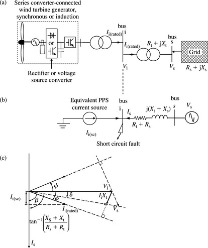
Figure 5.36 Modelling the short-circuit contribution of series converter-connected wind turbine generator: (a) initial prefault condition, (b) short-circuit fault condition and (c) vector diagram under fault conditions
Figure 5.36(a) shows a series converter-connected generator, which may be induction or synchronous, with the grid inverter connected through a transformer to a distribution voltage level of typically 20–36 kV This is then connected to a higher voltage system through another transformer. The largest pre short-circuit inverter current is that supplied at rated power and reactive power output of the inverter. Assume that at bus i the inverter rated power output is P, rated lagging reactive power output is Q and the rated lagging and (leading) power factor is cos φ. Thus, the rated inverter current delivered at bus i just before the short circuit is given by
The relationship between bus i voltage and system voltage Vs at bus s, ignoring the transformer resistance Rt, because it is much smaller than its reactance Xt, is given by
At bus s, the grid system is represented by its three-phase short-circuit infeed and Xs/Rs ratio. Since the grid inverter continues to supply a constant, balanced three-phase current during the short-circuit fault and the resultant voltage dip at its terminals, the inverter and its transformer can be represented as a constant PPS current source as shown in Figure 5.36(b). For a three-phase short-circuit fault at bus i, the PPS current supplied to the fault from the high voltage grid system is given by
 (5.138)
In practice, (Xs + Xt)/(Rs + Rt) will be dominated by the transformerXt/Rt ratio which is typically between 14 and 30. These correspond to impedance phase angles tan−1(Xt/Rt) of 86° and 88°, respectively. Figure 5.36(c) shows the vector diagram of the above voltages and currents including the system short-circuit current. The inverter PPS short-circuit current component that is in phase with Is is given by
For example, for Xt/Rt = 14.3 or tan−1(Xt/Rt) = 86°, rated inverter lagging power factor on the high voltage side of its transformer is 0.95 or φ = cos−1(0.95) = 18.2° and load angle δ = 6°, we have ![]() cos[86 - (18.2 - 6)] ≈ 0.28II(rated).
cos[86 - (18.2 - 6)] ≈ 0.28II(rated).
The total short-circuit current is the sum of the high voltage system and inverter short-circuit current contributions, i.e. ITotal = Is + Ii(sc).
If the inverter were operating at rated leading power factor, it can be shown that
However, in this case, although this current has a larger magnitude, it is in anti-phase with the dominant current supplied from the higher voltage system and will thus act to reduce the total short-circuit current. Equation (5.139) shows that the inherent inverter short-circuit current contribution is a small fraction of the inverter rated current.
Unlike a doubly fed induction generator, series converter-connected generators with a voltage sourced grid-side converter can provide a controlled short-circuit current response during the entire fault duration. Therefore, network utilities usually require a larger short-circuit current contribution from such generators to assist network protection in the detection of short-circuit currents. Therefore, modern grid-side inverter controls are usually designed to supply a larger and constant value of three-phase short-circuit current that is related to the rated current by
where α ≤ 3 for most current inverter designs.
As we have already explained, the inverter can be considered to act as a PPS constant current source during the entire short-circuit period as given by Equation (5.141). In addition, the inverter current control strategy ensures that the PPS short-circuit current supplied does not contain a dc current component.
Under unbalanced short-circuit faults in the network, e.g. a one-phase to earth short-circuit fault, the control systems of most modern inverters are designed to continue to supply balanced three-phase currents irrespective of the degree of their voltage unbalance. Therefore, under unbalanced short-circuit faults, the inverter will only supply a PPS current with the NPS and ZPS currents being equal to zero.
In summary, series converter-connected generators with grid-side inverters that deliver an increased constant current can be represented in short-circuit studies by a PPS constant current source, given by Equation (5.141), and zero NPS and ZPS current sources. It is generally incorrect to assume that the inverter PPS short-circuit current contribution can be represented as a voltage source behind a PPS reactance in pu equal to 1/α. This representation will produce the correct inverter current contribution for one fault location only namely at the inverter transformer output terminals. At other fault locations on the grid network, the voltage source representation will produce a lower and incorrect current than that given by Equation (5.141). The inverter constant current control strategy is normally very fast so that the ac short-circuit current contribution does not change with time during the short circuit. This means that the initial peak current and break current are equal.
[1] Kundur P. Power System Stability and Control. McGraw-Hill, Inc.; 1994. 0-07-035958-X.
[2] Krause P.C. Analysis of Electric Machinery. New York: McGraw-Hill; 1986.
[3] Adkins B., et al. The General Theory of Alternating Current Machines. Chapman and Hall; 1975. 0-412-15560-5.
[4] Concordia C. Synchronous Machines-Theory and Performance. New York: John Wiley; 1951.
[5] Kai T., et al. A simplified fault currents analysis method considering transient of synchronous machine. IEEE Transactions on Energy Conversion. September 1997;Vol. 12(No. 3):225-231.
[6] Hwang H.H. Transient Analysis of unbalanced short circuits of synchronous machines. IEEE Transactions on Power Apparatus and Systems. January 1969;Vol. PAS-88(No. 1):67-71.
[7] Hwang H.H. Mathematical analysis of double line to-ground short circuit of an alternator. IEEE Transactions on Power Apparatus and Systems. October 1967;Vol. PAS-86(No. 10):1254-1257.
[8] Kamwa I., et al. Phenomenological models synchronous machines from short-circuit test during commissioning—a classical/modern approach. IEEE Transactions on Energy Conversion. March 1994;Vol. 9(No. 1):85-97.
[9] Kamwa I., et al. Experience with computer-aided graphical analysis of sudden-short-circuit oscillograms of large synchronous machines. IEEE Transactions on Energy Conversion. September 1995;Vol. 10(No. 3):407-414.
[10] No. 2Canay I.M. Determination of model parameters of synchronous machines. Proceedings IEE. Vol. 130. March 1983:86-94.
[11] Luke Y.Y., et al. Motor contribution during three-phase short circuits. IEEE Transactions On Industry Applications. November/December 1982;Vol. 1A-18(No. 6):593-599.
[12] No. 1Kalsi S.S., et al. Calculating of system-fault currents due to induction motors. Proceedings IEE. Vol. 118. January 1971:201-215.
[13] No. 11Cooper C.B., et al. Application of test results to the calculation of short-circuit levels in large industrial systems with concentrated induction-motor loads. Proceedings IEE. Vol. 116. November 1969:1900-1906.
[14] Huening W.C. Calculating short-circuit currents with contributions from induction motors. IEEE Transactions on Industry Applications. March/April 1982;Vol. 1A-18(No. 2):85-92.
[15] Niiranen J. Voltage dip ride through of a doubly fed generator equipped with an active crowbar. In: Nordic Wind Power Conference. Sweden: Chalmers University of Technology; March 2004.
[16] Gertmar L., et al. New method and hardware for grid-connection of wind turbines and parks. Nordic Wind Power Conference. ESPOO, Finland. May 2006.