
6 Short-circuit analysis techniques in ac power systems
6.1 General
In modern power systems, there are various types of active sources that can contribute short-circuit currents in the event of short-circuit faults on the power system. These include synchronous and induction generators, synchronous and induction motors and modern power electronics converter connected generators. Power system elements such as lines, cables, transformers, series reactors, etc. between the short-circuit fault location and the various current sources will affect the magnitude of the short-circuit currents infeed into the fault. The effect is generally to reduce the magnitude of the short-circuit currents and to increase the rate at which their ac and dc components will decay.
In Chapter 1, we illustrated in Figure 1.4a the make and break duties of a circuit-breaker and explained their meanings. The calculation of these duties requires the calculation of the ac and dc components of the short-circuit current at the fault location in systems that generally contain many different short-circuit sources. Generally, published literature appears to cover the inherent current decay rate of a single source, generally that of synchronous machine, but not the decay rate in a real system that includes several or many sources. In addition, it is surprising that the analysis of the magnitude or rate of decay of the dc component of short-circuit current in a system that includes several or many sources has received virtually no attention in published power system analysis books. In this chapter, we will briefly analyse the effect of various network configurations on the time constants of the ac and dc components of short-circuit currents and hence the effect on the variation of their magnitudes with time. We will illustrate the effects of various estimation methods of the ac and dc time constants. We will then present some of the practical techniques that can be used in the analysis of the ac and dc components of short-circuit currents in interconnected power systems.
6.2 Application of Thévenin’s and superposition’s theorems to the simulation of short-circuit and open-circuit faults
6.2.1 Simulation of short-circuit faults
Thévenin’s and superposition’s theorems are very useful in the calculation of currents and voltages due to short-circuit faults in power system networks. The application of a short-circuit fault through a fault impedance ZF is represented by the closure of the switch between points F and F′ as shown in Figure 6.1(a).

Figure 6.1 Representation of short-circuit faults and prefault network: (a) short-circuit fault through a fault impedance by switch closure and (b) initial network condition before the short-circuit fault
The connection of a voltage source across the fault points FF′ equal in magnitude and phase to the prefault voltage, as shown in Figure 6.1(b), has no effect on the initial current and voltage conditions in the network. When the fault is applied, the voltage across the fault points FF′ drops to that across the fault impedance ZF i.e. to ZFIF or to zero for a solid fault where ZF = 0. This is represented by the connection of a second voltage source in series with ZF and the prefault voltage source as shown in Figure 6.2. The second voltage source is equal in magnitude but is 180° out of phase with the initial prefault voltage.

According to the superposition principle, the resultant currents and voltages in the network are the sum of those existed before the fault and the changes due to the fault itself. Therefore, using the superposition principle, the simulation of the short-circuit fault shown in Figure 6.2 is achieved by the sum of the voltages and currents from two separate networks namely those in Figures 6.1(b) and 6.3.
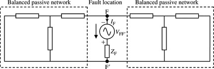
Figure 6.3 Calculation of current and voltage changes due to a short-circuit fault using Thévenin’s theorem
The first network, shown in Figure 6.1(b), is an active network representing the initial voltage and current conditions before the fault. The second network, shown in Figure 6.3, is a passive network apart from a single voltage source injected across the fault points FF′ with all other voltage sources in the rest of the network short-circuited. This is known as Thévenin’s network in which the calculated currents and voltages represent the current and voltage changes due to the fault. The final or actual currents and voltages are obtained by the superposition of the current and voltage results obtained from the two networks. The fault current flowing out of the network shown in Figure 6.3 into the fault at the fault location is given by
where ![]() is the Thévenin’s equivalent impedance of the entire network as ‘seen’ from between points FF′, φ is the Thévenin’s impedance angle, α is the initial prefault voltage angle, δ is the phase angle of ZThev. + ZF and β = α − δ is the fault current phase angle. The connection fault current between FF′ calculated from the passive network of Figure 6.3 is equal to the total fault current since the initial current is zero. The voltage change across the fault points FF′ due to the fault is calculated from Figure (6.3) as
is the Thévenin’s equivalent impedance of the entire network as ‘seen’ from between points FF′, φ is the Thévenin’s impedance angle, α is the initial prefault voltage angle, δ is the phase angle of ZThev. + ZF and β = α − δ is the fault current phase angle. The connection fault current between FF′ calculated from the passive network of Figure 6.3 is equal to the total fault current since the initial current is zero. The voltage change across the fault points FF′ due to the fault is calculated from Figure (6.3) as ![]() and the actual voltage during the fault is calculated using the superposition theorem from Figure 6.2 as
and the actual voltage during the fault is calculated using the superposition theorem from Figure 6.2 as
6.2.2 Simulation of open-circuit faults
The application of an open-circuit fault is represented by the opening of the switch between points F and F′ as shown in Figure 6.4(a).

Figure 6.4 Representation of open-circuit faults and initial network: (a) open-circuit fault by switch opening and (b) initial network condition before the open circuit
The connection of a current source across the fault points FF′ equal in magnitude and phase to the prefault current, as shown in Figure 6.4(b), has no effect on the initial currents and voltages in the network. When the open-circuit fault is applied, the current across the fault points FF′ drops to zero and this is represented by the connection of a second current source in parallel with the prefault current source. The second current source is equal in magnitude but is 180° out of phase with the initial prefault current as shown in Figure 6.5.

Using the superposition principle, the simulation of the open-circuit fault shown in Figure 6.5 is achieved by the sum of the voltages and currents from two separate networks as shown in Figures 6.4(b) and 6.6(a).
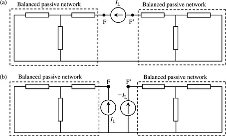
Figure 6.6 Calculation of current and voltage changes due to an open-circuit fault using Thévenin’s theorem: (a) series injected current source and (b) series injected current source replaced by two equal shunt injected current sources
The first network shown in Figure 6.4(b) is an active network representing the initial voltage and current conditions before the fault. The second network, shown in Figure 6.6(a), is a passive network apart from a single current source injected across the fault points FF′ with all other voltage sources short-circuited. The currents and voltages calculated as per Figure 6.6(a) represent the current and voltage changes due to the fault. The actual currents and voltages are obtained by the superposition of the currents and voltages obtained from the two networks. If the Thévenin’s equivalent impedance of the entire network as ‘seen’ from between points FF′ is equal to ZThév., the open-circuit voltage change across FF′ is given by
where IL′ is the known prefault current flowing from F to F′. The prefault voltage between FF′ is zero and hence the actual voltage across the open circuit is equal to that given in Equation (6.2).
An alternative representation to the series current source injected between points FF′ that is useful in practical large-scale analysis by matrix methods is shown in Figure 6.6(b). In this, the single injected series current source is replaced by two shunt injected current sources with that injected at F being equal to IL and that injected at F′ being equal to −IL.
6.3 Fixed impedance short-circuit analysis techniques
6.3.1 Background
Mathematically speaking, the meaning of impedance is only valid when the power system network is in a sinusoidal steady state. Further, as their name implies, fixed impedance analysis techniques assume that the impedance of every element in the power system network is constant. Obviously, this is the case for nearly all passive linear elements in the network, ignoring saturation, but, as we have seen in Chapter 5, the positive phase sequence (PPS) reactances of synchronous and induction machines are time dependent. The fixed impedance analysis technique assumes a constant fixed impedance value for every machine in the system such as X″d for synchronous machines and X″ for induction machines. The short-circuit current calculated is therefore the root mean square (rms) subtransient current at t = 0 or the instant of fault. The calculation may also be repeated using a different value for each synchronous machine impedance, usually, X′d. In this case, the short-circuit current calculated is the rms transient current and this may be considered in an empirical way to apply at a specific instant of time, such as 100 or 120 ms, in a meshed multi-machine network. Small induction machines forming part of the general power system load may or may not be represented depending on whether they will continue to provide a current contribution at this time. Some of the major international approaches to the representation of induction motor short-circuit current infeed will be covered in Chapter 7.
6.3.2 Passive short-circuit analysis techniques
The term passive short-circuit analysis means that the initial power system loading is ignored. The assumptions made are that the network voltage profile is uniform, transformer tap positions are nominal, and machine active and reactive power outputs are zero. No load currents flow in the network series branches, the shunt susceptances of network elements, e.g. lines, cables, capacitors, etc., as well as the shunt impedances of static load are not included in the network model. The calculated currents and voltages due to the application of the short-circuit fault are the changes that can be calculated as illustrated in Figure 6.3. The magnitude of the initial voltage at the fault location is usually taken as cUn where Un is the nominal system voltage and c is a voltage factor that is typically between 0.9 and 1.1 depending on whether maximum or minimum short-circuit currents are to be calculated. The voltage factor c is used in the international standard IEC 60909. This is discussed in Chapter 7.
6.3.3 The ac short-circuit analysis techniques
The term ac short-circuit analysis means that the initial power system load, i.e. magnitude and power factor, is taken into account prior to the application of the short-circuit fault. This is done using an ac loadflow study where the results are expressed in terms of machine active and reactive power outputs, transformer tap positions, voltage profile and load currents flowing in the network series branches. In the short-circuit study, the shunt susceptances of network elements, e.g. lines, cables, capacitors, etc., as well as the shunt impedances of static load may or may not be included in the network positive phase sequence (PPS), negative phase sequence (NPS) and zero phase sequence (ZPS) models depending on the approach adopted in a particular country. This is covered in Chapter 7. The calculated currents and voltages are obtained using the superposition theorem. The initial voltages and currents are taken from the initial loadflow study.
6.3.4 Estimation of dc short-circuit current component variation with time
Fixed impedance analysis enables the calculation of the ac component of short-circuit current at fixed time instants but the direct and explicit calculation of the dc component is obviously not possible. However, an estimate of the magnitude of the dc component at any time instant may be made in any type of network, i.e. radial or meshed by calculating the equivalent fixed impedance or Thévenin’s impedance at the fault point looking back into the active sources of currents. The inherent assumption made in this method is that the mathematical function describing the dc current at the fault point is that of a single decaying exponential with a single time constant, i.e. exp(−t/Tdc). The time constant Tdc is calculated from the equivalent system impedance ‘ seen’ at the fault point by dividing its reactance to resistance ratio X/R by ωs. The dc current magnitude can then be estimated at any required time instant. The accuracy of such a method is discussed in Sections 6.5.2 and 6.5.3.
In the case where passive short-circuit analysis techniques are used, as discussed in Section 6.3.2, the resistances of the network elements are included in the network model in order to calculate the equivalent system X/R ratio from the equivalent Thévenin’s impedance at the fault point. Alternatively, the equivalent system X/R ratio can be calculated from the Thévenin’s impedance phase angle φ as follows:
In some countries, e.g. in the American IEEE approach, the resistances of network elements may not be included in the network model used to calculate the current magnitude. Also, the equivalent X/R ratio at the fault point is calculated from separate reactance and resistance networks. The resistance network is obtained by setting all reactances to zero whereas the reactance network is obtained by setting all resistances to zero. An equivalent Thévenin’s resistance and another equivalent Thévenin’s reactance are calculated and the equivalent X/R ratio at the fault point is calculated as
The reason for calculating the X/R ratio of the dc component of short-circuit current using separate networks is to improve the accuracy of calculation. This is discussed in Chapter 7.
6.3.5 Estimation of ac short-circuit current component variation with time
As stated in Section 6.3.1 fixed impedance analysis enables the calculation of the ac component of short-circuit current at fixed time instants. For example, the subtransient and transient rms currents are calculated using the subtransient and transient reactances of machines, respectively. However, since the PPS reactances of synchronous and induction machines are time dependent, the ac component of fault current will in general vary with time, the extent of variation being dependent on the proximity of the fault to machines. In practical calculations, particularly where an appreciable proportion of the short-circuit current is supplied from nearby machines, e.g. on transmission networks and industrial power systems, the decay of the ac current is appreciable and this needs to be considered in the calculation of the make and break currents, of circuit-breakers.
The variation of the ac current is directly calculated when time domain analysis is used. However, with fixed impedance analysis, there is no direct analytical or theoretical approach that can be used, particularly in meshed networks. This will be further discussed in Section 6.5.
6.4 Time domain short-circuit analysis techniques in large-scale power systems
In general, the most accurate short-circuit current solution method should be capable of explicitly calculating the ac and dc components of short-circuit current at any time instant. If such accurate calculation is required, then time-step analysis techniques may be used. Conventional transient stability rms time-step simulations with the ability to model network unbalance, i.e. the PPS, NPS and ZPS networks allow for accurate calculation of the time variation of the ac component of short-circuit current. The main advantage of this approach is that the various ac short-circuit time constants of synchronous and induction machines and their impact on the ac fault current decay are accurately accounted for. However, this approach is generally impractical in large-scale short-circuit analysis in large power systems where 1000s of short-circuit studies are routinely carried out. The difficulties are generally the large data volume to be managed (although this is becoming less demanding in modern power system analysis programs with advanced data management facilities) and the significant computer running time requirements and hence the very long turn around time. Furthermore, in conventional transient stability analysis simulations, the dc component of short-circuit current is generally not calculated because the dynamic models of machines generally ignore the stator flux transients, i.e. in Chapter 5 in Equation (5.9), dψd/dt and dψd/dt are normally set to zero. Therefore, some other method would still be needed to calculate the dc current component.
Where an appropriate time domain analysis utilising time-step calculation is used, allowing the explicit calculation of the dc current component, it may be possible, if required, to estimate the dc component X/R ratio from the dc current waveform and dc current rate of decay.
6.5 Analysis of the time variation of ac and dc short-circuit current components
We recall that for a single short-circuit current source, i.e. a single machine, the machine short-circuit ac and dc time constants enable us to calculate the magnitudes of the ac and dc current components at any instant of time following the initial short-circuit fault instant. In this section, we limit our analysis to the most common types of short-circuit calculation, used for the assessment of substation infrastructure and circuit-breaker duties. These are three-phase and single-phase short-circuit faults.
6.5.1 Single short-circuit source connected by a radial network
The effect of a single short-circuit current source supplying a short-circuit current contribution to the fault through an external impedance was presented in Chapter 5. Essentially, the ac and dc short-circuit time constants are affected by the external impedance between the source and the fault point. To simplify the analysis, we assume that the external network impedance is predominantly reactive for the purpose of ac time constant calculation.
Figure 6.7 shows a single short-circuit source taken here as an unloaded synchronous generator having a star-connected stator winding with a solidly earthed neutral feeding into the fault point F through a radial link. This link may be one or more power system elements connected in series and have an equivalent series impedance of Re + jXe. From Chapter 5, the machine’s rms and dc short-circuit currents assuming a one per unit initial voltage are given by

Figure 6.7 Synchronous generator connected through a radial network to the short-circuit fault location
 (6.4a)
where XEq, the network ac and dc time constants for three-phase and single-phase short-circuit faults are given by
From Equations (6.4) and (6.5), we can determine the effect of a generator external impedance on the equivalent network ac and dc time constants, i.e. those of the fault current at the fault location, and hence on the time variation of the magnitude of the short-circuit current.
Effect of faults near to and far from short-circuit sources
The effect of electrical distance between the short-circuit source and the fault point on the initial magnitude of the short-circuit current, i.e. at the instant of fault is easily understood. The closer the fault location to the short-circuit source is, the smaller is the impedance between the source and the fault location, and the higher is the initial magnitude of short-circuit current. However, what is the effect on the magnitudes of the ac and dc currents afterwards, e.g. a few cycles later? To answer this question we need to understand, besides the effect on the current magnitude, the effect of the external impedance on the ac and dc time constants that govern the rates of decay of the ac and dc currents. This is an important aspect in practical short-circuit analysis. From Equations (6.4c) and (6.5), we have the following.
Three-phase short-circuit fault
 (6.6)
(6.6)The limiting values of the network subtransient time constant T″ac are determined by setting Xe = 0 and Xe → ∞ in Equation (6.6). Thus, the minimum value of T″ac is equal to T″d of the generator whereas the maximum value of T″ac is equal to
For most synchronous machines, ![]() to 1.5 X″d giving
to 1.5 X″d giving ![]() to 1.5T″d. However, because the difference between X′d and X′d is much smaller than that between X′d and Xd, the effect of external reactance on the initial magnitude of the subtransient component, as can be seen from Equation (6.4a), is much greater than the effect on the transient current component. In other words, the magnitude of the initial subtransient current component drops in a much greater proportion than the transient component. Following a similar approach for the network transient time constant T′ac given in Equation (6.4c), we have
to 1.5T″d. However, because the difference between X′d and X′d is much smaller than that between X′d and Xd, the effect of external reactance on the initial magnitude of the subtransient component, as can be seen from Equation (6.4a), is much greater than the effect on the transient current component. In other words, the magnitude of the initial subtransient current component drops in a much greater proportion than the transient component. Following a similar approach for the network transient time constant T′ac given in Equation (6.4c), we have
 (6.7)
(6.7)For most synchronous machines, Xd can be up to 8X′d thus T′ac ≈ T′d … 8T′d.
Similarly, the effect of the external reactance is to cause a proportionately much greater reduction in the transient current component than in the steady state current component. The network dc time constant Tdc given in Equation (6.4c) can be rewritten as
 (6.8)
(6.8)where Ta(3φ) is the generator’s armature time constant.
In practical power systems, generator X/R ratios X″d/Ra are significantly greater than the X″d/Ra ratios of external network elements Xe/Re of transformers, lines, cables, etc., or any combination of these. Therefore,
Thus, the effect of fault through an external impedance is to reduce the dc time constant and hence increase the rate of decay of the dc short-circuit current. The dc time constant is used to characterise the dc current component for circuit-breaker testing under IEC 62271–100:2001/2003 high voltage switchgear standard. In addition, it is usual power system practice to characterise the network dc current component by the network de X/R ratio given by
Figure 6.8 shows the variation of the ac component of short-circuit current for a near to generator three-phase short-circuit fault and a far from generator similar fault. The latter is separated from the generator terminal by a large external reactance. The important observation is that the ac current decay is very pronounced in the near to generator case but is negligible in the far from generator case. Conversely, the dc current decay is now greater than that for a generator alone.

Single-phase short-circuit fault
Similar analysis to the case of a three-phase short circuit can be carried out using Equations (6.4c) and (6.5). The reader is encouraged to show that similar conclusions to those for a three-phase short-circuit fault can be obtained.
The analysis approach of Section 6.5.1 can easily be applied to other short current sources such as synchronous motors, induction generators and motors.
6.5.2 Parallel independent short-circuit sources connected by radial networks
In this section, we present the effect of parallel short-circuit sources, each connected by a radial network, on the total short-circuit current ac and dc time constants and the variation of the current magnitude with time. Figure 6.9 shows n parallel short-circuit sources each feeding through its own external impedance to the fault point F.

Figure 6.9 n parallel synchronous generators each connected by a radial network to the short-circuit fault location
Network ac time constant
We consider the network subtransient ac time constant only since similar analysis also applies to the transient time constant.
In the case of a three-phase short circuit at point F, the total subtransient current component at F, using Equation (6.4a) is the sum of the subtransient current components supplied by each individual generator. Thus,
 (6.10a)
 (6.10b)
The expression for XEq in Equations (6.10a) and (6.10b) is a parallel equivalent and it ensures that the initial current magnitude, i.e. at t = 0, of the single equivalent exponential in Equation (6.10a) is equal to that obtained from the sum of the individual exponentials.
In the general case, sources have different impedances and time constants and each current component decays at a different rate. Therefore, the magnitudes of the n subtransient current components for t > 0 will be different. The same observation would be made even if the machines were identical, i.e. have similar parameters, but their external impedances were different. Consequently, a single network ac time constant at the fault location for all the ac sources that enables the calculation of the total current magnitude for t > 0 does not exist. Mathematically speaking, the sum of several exponentials of different time constants cannot be made equal to a single equivalent exponential with a single equivalent time constant. However, in this radial network topology this is not required because each source is radially connected to the fault point and the accurate equation for the sum of n exponential terms can be used. It can be shown that similar conclusions apply for single-phase short-circuit faults.
Network dc time constant
In the case of a three-phase short circuit at point F in Figure 6.9, the total dc current component at point F, using Equation (6.4b), is the sum of the dc current components supplied by each individual machine. Thus
 (6.11a)
 (6.11b)
Equation (6.11a) shows that at t = 0, the magnitude of the total dc current is equal to the sum of the magnitudes of the individual dc current components. However, for t > 0, and because each current component decays at a different rate, a single equivalent exponential component that gives an equivalent rate of decay or time constant for the sum of the individual exponentials does not exist. This is best illustrated in the following example.
Example 6.1
Consider three parallel sources or n = 3 in Figure 6.9 having significantly different time constants as follows: Tdc(1) = 50 ms, Tdc(2) = 150 ms and Tdc(3) = 15 ms. Using Equation (6.11b), the corresponding initial dc current magnitudes supplied at t = 0 by the three sources are equal to Idc(1) = 0.6 pu, Idc(2) = 0.3 pu and Idc(3) = 0.1 pu. These initial current magnitudes and their associated dc time constants can represent a variety of sources and external impedances such as synchronous machines, induction machines and equivalent infeeds from transmission or distribution networks. Figure 6.10 curve (a) shows the total dc fault current at point F supplied by the three parallel sources and calculated using Equation (6.11a), i.e. from the accurate sum of three exponential terms. Figure 6.10 also shows the total dc current derived from a single time constant as calculated by two different approximate methods. The first, curve (b), is calculated from the single X/R ratio of the equivalent impedance ‘seen’ at the fault point, ZThév. = R + jX, also known as IEC 60909 Standard Method B (this is discussed in Chapter 7). The second, curve (c), is calculated from the ratio of the equivalent reactance at the fault point, XThév., (with all resistances set to zero) to the equivalent resistance at the fault point, RThév., (with all reactances set to zero), as per IEEE C37.010 Standard (this is discussed in Chapter 7). It can be shown that the single equivalent time constant at the fault point using the IEC method is equal to 48.6 ms (X/R = 15.2 at 50 Hz). Using the IEEE method, the single equivalent time constant at the fault point is equal to 76.3 ms (X/R = 24.0 at 50 Hz). The equations for the dc currents calculated by the three methods are given by where t is in ms. Figure 6.10 shows that the IEC Method B single equivalent time constant underestimates the actual dc current for t ≥ 10 ms and this underestimate increases with time. Conversely, and because the IEEE RThév. is significantly smaller than the equivalent resistance calculated using the IEC approach, the IEEE time constant is 1.57 times the IEC time constant. Figure 6.10 shows that the IEEE approach, in this example, significantly overestimates the actual dc current over the period up to 140 ms, then the overestimate disappears. It should be noted that the degree of underestimate of IEC Method B and overestimate of IEEE Method varies with the initial magnitude of each current source and the relative time constants between them. Larger and smaller underestimates and overestimates can be found in practice and the reader is encouraged to analyse the effect of different combinations.

Figure 6.10 Illustration of IEC and IEEE approaches for the calculation of dc short-circuit current variation with time for Figure 6.9
6.5.3 Multiple short-circuit sources in interconnected networks
The topologies of transmission, subtransmission and many distribution power systems are such that multiple sources of short-circuit currents feed into the short-circuit fault via a meshed or interconnected network topology. For most practical networks, the effect of multiple short-circuit sources supplying currents through a meshed network configuration on the ac and dc time constants of the short-circuit current at the fault location is not amenable to analytical treatment. However, understanding this effect is of vital importance in practical short-circuit calculations if significant inaccuracies are to be avoided. The analysis presented next will explain the problem.
Network ac time constant
Figure 6.11(a) shows a simple meshed network that consists of three independent short-circuit current sources, each is connected by an external impedance to a common node N. The three sources are then connected to the short-circuit fault location F via a common impedance. To illustrate the problem, each source is assumed to be a synchronous machine whose time-dependent reactance is given by

Figure 6.11 Simple meshed network for the analysis of ac short-circuit current decrement (variation with time): (a) network configuration and (b) equivalent circuit
 (6.12)
The equivalent circuit is shown in Figure 6.11(b) where each machine is replaced by a constant voltage source Eo behind its time-dependent PPS reactance, given by Equation (6.12), and the armature resistance. The equivalent time-dependent
PPS system impedance at the fault point F is given by
 (6.13)
From Equation (6.13), it is interesting to note that not only the equivalent reactance XF at the fault point is time dependent but also the equivalent resistance RF. In many practical calculations, we can assume that Xm(i)(t) + X(i)(t) » (Rai + Ri) for i = 1, 2 and 3, and Xc » Rc. Therefore, from Equation (6.13), we have
In general, the magnitude of the time-dependent ac component of fault current at the fault point F is given by
The substitution of Equation (6.12) in Equation (6.13) or (6.14) shows that the fault current magnitude given by Equation (6.15) would still exhibit subtransient and transient decay. However, the corresponding time constants are very complicated functions of the three individual machine time constants and no general analytical formula can be derived. The accuracy of various methods of calculating the time variation of the ac short-circuit current component is illustrated using an example.
Example 6.2
Consider Figure 6.11. The three machines are generators having the following parameters: Xd = 2.04 pu, X′d = 0.275 pu, X′d = 0.19 pu, T′d = 40 ms, T′d = 1100 ms, X1 = X2 = X3 = 0.19 pu, Xc = 0.2 pu.
Curve (a) of Figure 6.12 shows the accurate time variation of the magnitude of the rms short-circuit current obtained from Equation (6.15b) with Eo = 1 pu. Curve (b) shows the current waveform obtained from the Thévenin’s equivalent subtransient, transient and steady state impedances calculated at the fault point F as X″F = 0.3267 pu, X′F = 0.355 pu and XF = 0.9434 pu, respectively. The subtransient and transient time constants that include the effect of each machine’s external impedance up to node N but exclude the effect of the common impedance Zc are calculated as T″de(i) = 47.3 ms and T′de(i) = 1701.5 ms. X″F, X′F and XF are calculated usingX″d(i), X′d(i) and Xd(i), respectively, for each machine. The current obtained by using the Thévenin’s equivalent subtransient, transient and steady state impedances is given by,

Figure 6.12 Illustration of different approaches for the calculation of ac short-circuit current variation with time for a meshed network
As expected, curve (b) Equation (6.16) underestimates the current magnitude for t > 0 and this underestimate increases with time. The reason is that the common impedance Zc between node N and the fault point F will also cause some increase in the effective time constants of each source but Equation (6.16) fails to capture this effect. Curve (c) of Figure 6.12 shows the current variation if maximum known values of practical synchronous machine transient and subtransient time constants are used in Equation (6.16). These are 2000 and 70 ms, respectively. The result shows a small overestimate of up to around 90 ms, then an increasing underestimate thereafter. If the time range of interest is up to around 120 ms, as would be the case in high voltage and extra high voltage systems, then an approximation can be made in Equation (6.16) by setting ![]() Also, using an average value for synchronous machine subtransient time constants of around 40 ms, we can write
Also, using an average value for synchronous machine subtransient time constants of around 40 ms, we can write
Equation (6.17) is plotted as curve (d) in Figure 6.12 where the current falls to the minimum transient value then remains constant. Equation (6.17) gives an increasing overestimate with time for t ≥ 50 ms.
The above analysis can easily be extended to single-phase short-circuit faults using the machine time-dependent PPS reactance equations derived in Chapter 5.
There is no international consensus on how to calculate the time variation of the ac component of short-circuit current in practical meshed networks, when fixed impedance analysis techniques are used. Different empirical approaches are used, and this will be covered in Chapter 7.
Network dc time constant
We will continue to use the meshed network topology shown in Figure 6.11(a), but to simplify the analysis, we now use constant voltage sources instead of synchronous machines. The voltage source equation is given by ![]() When a short-circuit fault occurs at point F, the time domain solution of the short-circuit currents supplied by each source and the total fault current can be obtained by replacing all reactances with corresponding inductances and writing the differential equations relating the currents and voltages in this network. We encourage the reader to carry out this simple but time consuming exercise in Kirchoff’s voltage and current laws to obtain the solutions of the four currents. It can be shown that the instantaneous short-circuit current supplied by each voltage source and the total short-circuit current at the fault point F are given by
When a short-circuit fault occurs at point F, the time domain solution of the short-circuit currents supplied by each source and the total fault current can be obtained by replacing all reactances with corresponding inductances and writing the differential equations relating the currents and voltages in this network. We encourage the reader to carry out this simple but time consuming exercise in Kirchoff’s voltage and current laws to obtain the solutions of the four currents. It can be shown that the instantaneous short-circuit current supplied by each voltage source and the total short-circuit current at the fault point F are given by

All the constant multipliers and the three dc time constants are complicated functions of the network resistances and inductances.
Equation (6.18b) shows that the dc component of the total short-circuit current consists of three components having different time constants Tdc(1), Tdc(2) and Tdc(3). The following example compares the accurate solution against the methods of characterising the dc current by a single decaying exponential having a time constant derived from the IEC 60909 Method B and the IEEE C37.010 approaches.
Example 6.3
In Figure 6.11(a), the X/R ratios of the four network branches are as follows: X1/R1 = 15.7, X2/R2 = 47.0, X3/R3 = 4.7, Xc/Rc = 10. Figure 6.13 shows that, as in the case of parallel independent sources, the equivalent X/R ratio at the fault point or single exponential method underestimates the true magnitude of the dc current component. However, the underestimate produced using the IEC Method B is generally smaller in meshed network than that produced in a network having parallel independent sources, due to the common impedance branch that is shared by the three sources in the meshed network. The configuration of parallel independent short-circuit sources generally produces the worst case underestimate. An overestimate is observed using the IEEE C37.010 Method. The errors in the dc currents calculated using the IEC and IEEE approaches on one hand and the accurate solution reduce with increasing Zc that is increasing distance between the machines and the fault location. In other words, as Zc increases, the IEC and IEEE curves move towards the curve that represents the accurate solution. Although we have used simple parallel and meshed network configurations to present the problem of dc current estimation, the conclusions regarding the errors observed in such network configurations are generally applicable in other networks.

Figure 6.13 Illustration of IEC and IEEE approaches for the calculation of dc short-circuit current variation with time for Figure 6.11(a)
6.6 Fixed impedance short-circuit analysis of large-scale power systems
6.6.1 Background
Fixed impedance analysis allows the direct calculation of the rms value of the ac component of short-circuit current using phasor algebra. Hand calculations play a useful and important role in gaining an insight into problems. However, these can only be used in problems of low dimensionality. General analysis methods using matrix algebra suitable for digital computer calculations are almost universally used. Our presentation will be of practical nature that allows the inclusion, as required, of some or all of the following: resistive elements of series impedances, shunt capacitance of lines and cables, transformer magnetising reactances, transformer actual off-nominal tap positions determined from an initial loadflow study, shunt reactors and capacitors, etc. The sequence interconnection networks of various faults developed in Chapter 2 and the sequence models of various power plants developed in Chapters 3–5Chapter 4Chapter 5 are used to formulate a sequence model of the entire network. In this section, we will present a brief overview of the type of general analysis techniques that are directly applicable to large-scale N bus systems.
6.6.2 General analysis of balanced three-phase short-circuit faults
Thévenin’s and Norton’s PPS equivalent of models of machines
The topology of power system networks and the data of all network elements, as well as the initial network loading and generation operating conditions, allow the formation of a nodal equivalent network of admittances and injected current sources. Short-circuit current sources such as generators and, where required, motors can be represented at the time instant of interest as constant voltage sources behind the appropriate machine fixed impedance, e.g. subtransient or transient impedance or any another value, as appropriate. Figure 14.6(a) and (b) shows equivalent models of a loaded synchronous machine. The latter shows a nodal or Norton’s equivalent which consists of a current source in parallel with the machine admittance.
From Figure 6.14(a), the apparent power output of a machine connected to node (i) is given by

The short-circuit current supplied by the machine for a fault at node i is given by
Using Em(i) from Equation (6.19a) in Equation (6.19b), we obtain
PPS admittance and impedance matrix equations
Figure 6.15 shows a simple power system network that will be used to illustrate the process of formulating the sequences nodal matrices.

The formation of the admittance matrix starts by forming the positive sequence nodal model shown in Figure 6.16, where each network element is replaced by its PPS model.

Figure 6.17 shows the nodal equivalent model with all shunt elements at every node collected into an equivalent shunt branch. The result is only one shunt branch at each node and a series branch interconnecting two nodes. The nodal admittance matrix equation of the resultant nodal equivalent circuit is given by

 (6.20a)
The admittance matrix of Equation (6.20) is in general symmetric, and even for small power systems, it is quite sparse, i.e. it contains only a few non-zero elements, each representing an admittance element connecting two nodes. For example, for a medium size system of 4000 nodes and 3000 series branches, the number of non-zero elements is 4000 + 2 × 3000 = 10 000. This is only 0.0625% of the total number of elements of the full matrix (4000 × 4000 = 16000000).
The use of the nodal admittance matrix in calculating short-circuit currents is inefficient, as it requires a new solution for each fault location and fault type. Therefore, the nodal impedance matrix given in Equation (6.21) below is used. It is important to note that the current vector represents a set of injected nodal current sources. Thus, from Equation (6.20b),
 (6.21b)
The nodal impedance matrix is generally full, i.e. it contains elements in every position unless there are disconnected parts of the network, as would be the case in the ZPS network as we discuss later. However, in practice, it is inefficient to obtain this matrix by direct inversion of the admittance matrix for medium and large size systems. Direct inversion of large matrices is avoided by the use of various computer-based numerical calculation techniques, such as the method of successive forward elimination and backward substitution (also known as Gaussian elimination). Other similar methods are also used, such as Kron reduction, triangular factorisation, LU decomposition and others. Generally, the sparse admittance matrix can be retained and the impedance matrix is calculated or built directly from the factorised admittance matrix.
Referring back to Equation (6.21b), it is important to appreciate the meaning of the diagonal and off-diagonal elements of the nodal impedance matrix. The diagonal terms ![]() , with all other current sources set to zero, is termed the driving point impedance or the Thévenin’s impedance as ‘seen’ from node k. This impedance is equal to the voltage produced at node k divided by the current injected at node k. The off-diagonal terms are, for example,
, with all other current sources set to zero, is termed the driving point impedance or the Thévenin’s impedance as ‘seen’ from node k. This impedance is equal to the voltage produced at node k divided by the current injected at node k. The off-diagonal terms are, for example, ![]() again with all other current sources set to zero is termed the transfer impedance between nodes 1 and k. It is equal to the voltage produced at node 1 divided by the current injected at node k.
again with all other current sources set to zero is termed the transfer impedance between nodes 1 and k. It is equal to the voltage produced at node 1 divided by the current injected at node k.
General analysis of three-phase short-circuit faults
We will present a general analysis technique suitable for the calculation of not only the short-circuit current at the fault location but also the currents and voltages throughout the network. As explained in Section 6.3.2, the application of the fault will cause current and voltage changes in the network. The calculation of these quantities in a large-scale system of N nodes makes use of the efficiently calculated nodal bus impedance matrix of the system. Since the three-phase short circuit is a balanced fault, the system nodal admittance and nodal impedance matrices are in effect PPS admittance/impedance matrices since all the network elements are replaced by their PPS models. The actual currents and voltages in the network due to the fault are obtained by the superposition of the initial currents and voltages and the Thévenin’s changes. Thus,
Three-phase short-circuit fault at one location
Denote the faulted node as k, the fault impedance as ZF, the connection fault current as IF, the Thévenin’s impedance at node k as Zkk and the prefault voltage at node k as Vk(o). The calculation of the current and voltage changes at the fault location and elsewhere is illustrated using Figure 6.18 and the nodal bus impedance matrix of Equation (6.21b).
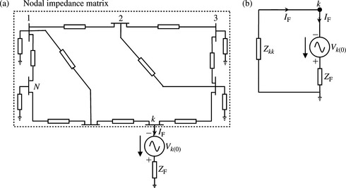
Figure 6.18 Calculation of current and voltage changes using Thévenin’s equivalent circuit: (a) representation of the entire network and (b) equivalent at the faulted node k
Since we are considering a fault at one location only, namely node k, there is only one injected node current Ik = −IF and all other injected currents are zero. Therefore, from Equation (6.21b), the voltage changes are given by
 (6.23a)
From Equation (6.23a), the voltage changes caused by the fault are given by
 (6.23b)
The actual voltage during the fault at the faulted node k is given by
From Equation (6.23b) row k, we can write ![]() and using Equation (6.24), we obtain
and using Equation (6.24), we obtain
Having calculated the fault current, the nodal voltage changes throughout the network are calculated using Equation (6.23b). The changes in branch currents are calculated from the nodal voltage changes using
where yij is the retained admittance of branch ij.
Denoting the actual nodal voltages during the fault as V1, Vk … VN, then from Equation (6.23b), we can write
 (6.27)
Substituting Equation (6.25) in Equations (6.24) or (6.27), the actual nodal voltages can be expressed as
For a solid short-circuit fault, ZF = 0. The actual branch currents are calculated using
The short-circuit current contribution of each machine is calculated from the actual nodal voltages where each machine is connected and using Equation (6.19c)
or, alternatively, using Equation (6.19b) in Equation (6.31)
Simultaneous three-phase short-circuit faults at two different locations
In Figure 6.19(a), denote the faulted nodes as j and k, the corresponding fault impedances as Zj(F) and Zk(F) and the connection fault currents as Ij(F) and Ik(F). The Thévenin’s impedances at nodes j and k are Zjj and Zkk, the transfer impedances between nodes j and k are Zjk and Zkj and the prefault voltages at nodes j and k are Vj(o) and Vk(o).

Figure 6.19 Calculation of current and voltage changes for two simultaneous short-circuit faults using Thévenin’s equivalent circuits: (a) representation of the entire network for two simultaneous short-circuit faults and (b) equivalent between faulted nodes j and k
From Equation (6.21b), we can write
 (6.33)
Since the nodal impedance matrix is symmetric, Zjk = Zkj. Therefore, the voltage changes in Equation (6.33) caused by the faults are given by
 (6.34)
The actual voltages during the faults at the faulted nodes j and k are given by
From Equation (6.34) rows j and k, we can write
Substituting Equations (6.35a) and (6.35b) in Equations (6.36a) and (6.36b), respectively, and solving for the fault currents, we obtain
It is instructive to visualise the Thévenin’s equivalent circuit seen from the two faulted nodes j and k. Adding and subtracting ZjkIj(F) to Equation (6.36a) and ZjkIk(F) to Equation (6.36b), we obtain
Equations (6.35) and (6.38) can be represented by the equivalent circuit shown in Figure 6.19(b). As expected, the Thévenin’s impedance from nodes j and k to earth, or to the reference node, are Zjj and Zkk, respectively. The equivalent Thévenin’s impedance between the faulted nodes j and k is given by
Having calculated the fault currents using Equation (6.37), the nodal voltage changes are calculated using Equation (6.34). The actual voltages are then calculated using Equation (6.22a). The actual branch and machine currents are calculated using Equations (6.30) and (6.32), respectively.
Three-phase short-circuit fault between two nodes
In Figure 6.20(a), consider a fault between nodes j and k. The fault impedance is ZF, the connection fault currents are Ij(F) and Ik(F), the Thévenin’s impedances at nodes j and k are Zjj and Zkk, the transfer impedance between nodes j and k is Zjk = Zkj, and the prefault voltages at nodes j and k are Vj(o) and Vk(o). Consider the fault current to flow out of node j and into node k hence the injected currents are Ij(F) = −I(F) and Ik(F) = I(F).

Figure 6.20 Representation of a three-phase short-circuit fault between two nodes: (a) Thévenin’s representation of the entire network and (b) Thévenin’s equivalent between nodes j and k for a short-circuit fault between them
From Equation (6.21b), we can write
 (6.40)
From Equation (6.40), the voltage changes caused by the fault are given by
 (6.41)
The actual voltage during the fault between the faulted nodes j and k is given by
From Equation (6.41) rows j and k, we can write
From Equations (6.42) and (6.43), the fault current is given by
Equations (6.42) and (6.44) are represented by the Thévenin’s equivalent circuit shown in Figure 6.20(b). Having calculated the fault current, the nodal voltage changes are calculated using Equation (6.41). The actual voltages are then calculated using Equation (6.22a). The actual branch and machine currents are calculated using Equations (6.30) and (6.32), respectively.
6.6.3 General analysis of unbalanced short-circuit faults
Nodal sequence impedance matrices
In the case of a three-phase short circuit, only the PPS nodal impedance matrix is required, as presented in Section 6.6.2. For a two-phase unbalanced short circuit, the NPS nodal impedance matrix is also required. This can be efficiently derived from the NPS nodal admittance matrix, as we discussed for the PPS impedance matrix. From the early days of digital computer analysis of large power systems, an assumption has generally been made that the NPS and PPS impedance matrices are identical in order to remove the need to form, store and calculate the NPS nodal matrix. This is based on the assumption that the PPS and NPS models and parameters of all passive network elements are identical and that those for machines do not differ significantly. However, this assumption is only approximately valid when calculating the subtransient short-circuit current using machine subtransient impedances. It is not valid when calculating the short-circuit current some time after the instant of fault, e.g. the transient current using machine transient impedances, because these differ significantly from the machine NPS impedances. On the whole, with the huge and cost-effective increases in computing storage and speed, particularly since the early 1990s, this assumption is no longer needed.
In the case of a single-phase to earth and two-phase to earth faults, the nodal ZPS impedance matrix is also required in addition to the PPS and NPS impedance matrices. This matrix is radically different from the PPS and NPS impedance matrices both in connectivity due to e.g. transformer windings and impedance values of most network elements. Figure 6.21 shows the ZPS network model of Figure 6.15.

General fault impedance/admittance matrix for unbalanced short-circuit faults
It is useful to derive a single method of analysis that covers all unbalanced short-circuit faults, namely single-phase to earth, two-phase and two-phase to earth. Such a method needs to allow for both solid short circuits and those through fault impedances. Figure 6.22 shows a general fault connection node with four impedances or admittances, the values of which can be appropriately chosen to represent any type of unbalanced short circuit.

It can be shown that the phase voltages and currents at the fault location are related by the following equation:
 (6.45a)
and the fault impedance matrix is defined as
 (6.45b)
For example, to represent a solid single-phase to earth fault, we set ZR = 0, ZE = 0, ZY = ∞ and ZB = ∞. Similarly, we represent a solid two-phase (Y-B) short circuit by setting ZY = 0, ZB = 0, ZR = ∞ and ZE = ∞. The sequence fault impedance matrix is calculated using ![]() The result is given by
The result is given by
 (6.46)
However, as we have already seen, some of the impedances will be infinite under certain fault conditions and as a result ![]() will become undefined. This problem
will become undefined. This problem
is solved by inverting ![]() to obtain the sequence fault admittance matrix as follows:
to obtain the sequence fault admittance matrix as follows:
 (6.47)
Single-phase to earth short circuit through a fault impedance ZF
As already outlined, this case is produced by setting ZR = ZF or YR = 1/ZF, ZE = 0 or YE = ∞ and ZY = ZB = ∞ or YY = YB = 0. Therefore, the elements of Equation (6.46) are infinite and the sequence impedance matrix is thus undefined. However, Equation (6.47) results in indeterminate expressions which can be reduced to the following:
 (6.48)
Two-phase short circuit through a fault impedance ZF/2
This case is produced by setting ZY = ZB = ZF/2 or YY = YB = 2/ZF, ZE = ∞ or YE = 0 and ZR = ∞ or YR = 0. Therefore, the elements of Equation (6.46) are infinite and the sequence impedance matrix is thus undefined. However, Equation (6.47) results in the following useful matrix:
 (6.49)
Two-phase to earth short circuit through a fault impedance ZF and earth impedance ZE
This case is produced by setting ![]() or
or ![]() or YR=0. Where the earth impedance is equal to zero, ZE = 0, YE = ∞. Therefore, the elements of Equation (6.46) are infinite and the sequence impedance matrix is consequently undefined. However, Equation (6.47) results in the following useful matrix:
or YR=0. Where the earth impedance is equal to zero, ZE = 0, YE = ∞. Therefore, the elements of Equation (6.46) are infinite and the sequence impedance matrix is consequently undefined. However, Equation (6.47) results in the following useful matrix:
 (6.50a)
where the earth impedance ZE is finite, Equation (6.47) results in the following:
 (6.50b)
General mathematical analysis
Using Thévenin’s theorem, and Equation (6.22b) the current and voltage changes in the PPS, NPS and ZPS networks, dropping the delta sign for currents for convenience, are given by
where ![]() and
and ![]() are the PPS, NPS and ZPS nodal impedance matrices, respectively, of the N node network. Prior to the short-circuit fault, the NPS and ZPS currents between all nodes, and the NPS and ZPS voltages at all nodes are zero because the three-phase system is assumed to be balanced. Where the system loading or operating condition is to be taken into account, the PPS voltages and currents are obtained from an initial loadflow study. Therefore, using the superposition principle, the actual nodal voltages during the fault are given by
are the PPS, NPS and ZPS nodal impedance matrices, respectively, of the N node network. Prior to the short-circuit fault, the NPS and ZPS currents between all nodes, and the NPS and ZPS voltages at all nodes are zero because the three-phase system is assumed to be balanced. Where the system loading or operating condition is to be taken into account, the PPS voltages and currents are obtained from an initial loadflow study. Therefore, using the superposition principle, the actual nodal voltages during the fault are given by
 (6.53a)
 (6.53b)
The short-circuit fault is applied at node k. Thus, all injected sequence currents in the three sequence networks are zero except the sequence currents injected at the faulted node k. Equations (6.53a) and (6.53b) become
 (6.54a)
 (6.54b)
From Equations (6.52) to (6.54), we can extract the sequence voltage components of row k as follows:
 (6.55a)
 (6.55c)
The PPS, NPS and ZPS networks are interconnected at the fault location in a manner that depends on the fault type, as described in Chapter 2. For the general analysis of any type of unbalanced fault, in fact even balanced faults if desired, we need to describe the conditions at the fault location using a general method. One method is to use of a fault admittance matrix that is dependent on the fault type, as described in the previous section. Thus, the sequence fault currents can be written as
Substituting Equation (6.56) into Equation (6.55b), we obtain
where U is the identity matrix. The sequence fault currents at the faulted node k are now obtained by substituting Equation (6.57) back into Equation (6.56), giving
The sequence voltages at the faulted node k, ![]() , are calculated using Equation (6.57). The PPS, NPS and ZPS voltages throughout the PPS, NPS and ZPS networks can be calculated by substituting Equation (6.54) in Equation (6.52). Therefore, for a fault at node k, the sequence voltages at any node i are given by
, are calculated using Equation (6.57). The PPS, NPS and ZPS voltages throughout the PPS, NPS and ZPS networks can be calculated by substituting Equation (6.54) in Equation (6.52). Therefore, for a fault at node k, the sequence voltages at any node i are given by
 (6.59)
The actual sequence currents flowing in the branches of the PPS, NPS and ZPS networks are calculated as follows:
 (6.60)
The sequence current contributions of each machine are calculated as follows:
 (6.61)
Having calculated the sequence components of every nodal voltage and branch current, the corresponding phase voltages and currents are calculated using VRYB = HVPNZ and IRYB = HIPNZ, where H is the transformation matrix given in Chapter 2. The reader should remember to modify the phase angles of the sequence currents and voltages in those parts of the network which are separated from the faulted node by star-delta transformers, as discussed in Chapter 4.
6.6.4 General analysis of open-circuit faults
One-phase open-circuit fault
The connection of the PPS, NPS and ZPS sequence networks was covered in Chapter 2, and shown in Figures 2.10 and 2.11 for one-phase and two-phase open-circuit faults, respectively. In these figures, the PPS, NPS and ZPS impedances are the Thévenin’s impedances seen looking from the open-circuit fault points F and F′. We first illustrate how these impedances are calculated making use of the nodal impedance matrix and the Thévenin’s impedance between two nodes using Figure 6.23.

In Figure 6.23, consider an open-circuit fault on a circuit connected between two nodes j and k and having sequence impedances ZP, ZN and ZZ. In Equation (6.39), we derived the equivalent Thévenin’s impedance between two nodes j and k and showed it in Figure 6.19(b). This Thévenin’s impedance includes the circuit that is physically connected between nodes j and k. An open-circuit fault can be represented by removing the circuit between nodes j and k completely, i.e. all three phases, and then reinserting the appropriate sequence impedances ZP, ZN and ZZ of the circuit. The disconnection of the circuit can be simulated by connecting −ZP, −ZN and −ZZ between nodes j and k in the PPS, NPS and ZPS Thévenin’s equivalents. Therefore, the equivalent Thévenin’s impedance between the open-circuit points F and F′ is calculated as illustrated in Figure 6.24 and is given by

Figure 6.24 Calculation of (a) PPS, (b) NPS and (c) ZPS Thévenin’s impedances between open-circuit points F and F′
 (6.62a)
where, using Equation (6.39),
The prefault current flowing between F and F′ at node j before the open-circuit fault occurs is a PPS current, and is calculated from the initial loadflow study using
Alternatively, an approximate value may be calculated as follows:
Therefore, Equation (6.62) and the prefault current can be used in the equations derived in Chapter 2 for one-phase open circuit and two-phase open circuits to calculate the sequence currents and voltages at the fault location FF′.
To calculate the sequence voltage changes throughout the PPS, NPS and ZPS sequence networks using their nodal impedance matrices, we need to calculate the equivalent sequence currents to be injected at nodes j and k in each sequence network. These are easily calculated from Figure 6.24 by replacing each sequence voltage Vx in series with the circuit impedance Zx (x = P, N or Z) with a current source equal to Vx/Zx in parallel with Zx, the latter cancelling out when combined with −Zx. This current source Vx/Zx flows from node k to node j and can be considered as two separate current sources. The first is equal to Vx/Zx and is injected into node j, and the second is equal to −Vx/Zx and is injected into node k. Figure 6.25 illustrates the sequence current sources injected into each sequence network. In summary, the sequence current sources injected into nodes j and k are given by

Figure 6.25 Representation of open-circuit faults by injection of PPS, NPS and ZPS current sources into respective sequence networks
From Equations (6.51) and using x = P, N or Z, we have
 (6.65)
Using Equation (6.64), we obtain
 (6.66)
The actual NPS and ZPS sequence voltages are equal to the changes calculated using Equation (6.66), as shown in Equations (6.52b) and (6.52c). The actual PPS voltages are calculated by adding the prefault voltages obtained from the initial loadflow study to the PPS voltage changes calculated using Equation (6.66), as shown in Equation (6.52a). The actual sequence currents flowing in the branches of the PPS, NPS and ZPS networks are calculated using Equation (6.60).
6.7 Three-phase short-circuit analysis of large-scale power systems in the phase frame of reference
6.7.1 Background
In some detailed short-circuit studies, fixed impedance analysis using three-phase modelling of the power system is used. One reason for this is to correctly include the inherent network unbalance, such as that due to untransposed overhead lines and cables. Another reason is the need to correctly calculate the earth return currents which requires the calculation of currents flowing through the earth wires of overhead lines and through cable sheaths. Such calculations require the explicit modelling of the earth wire and sheath conductors. The representation of all conductors of an overhead line or cable necessitates the use of three-phase models. Thus, three-phase modelling and analysis is then carried out in the phase frame of reference, since the symmetrical components sequence reference frame loses its advantages. In Chapter 3, we presented three-phase modelling of overhead lines and cables, and in Chapter 4, we presented three-phase modelling of transformers and other static power plant. In this section, we present a three-phase model of a current source, e.g. a synchronous machine and a general three-phase short-circuit analysis technique in the phase frame of reference that can be used in large-scale power systems.
6.7.2 Three-phase models of synchronous and induction machines
In Figure 6.14, we presented a PPS machine model using Thévenin’s and Norton’s equivalents. From Chapter 5, we know that an ac machine will also present an NPS impedance to the flow of NPS current. Whether a ZPS impedance is presented to the flow of ZPS currents depends on the stator winding connection and earthing method.
Synchronous machines
To maintain generality, we assume that, the synchronous machine NPS impedance is not equal to the PPS impedance. From the three independent sequence networks of the machine, shown in Figure 6.26, the following sequence equation can be written

 (6.67a)
Before the short-circuit fault occurs, the machine is assumed to produce a balanced set of three-phase voltages having a PPS component only. However, the machine may be assumed to be connected to either a balanced or an unbalanced network. If the network is balanced, then only PPS currents flow, but if the network is unbalanced, then NPS and ZPS currents will also flow. Multiplying Equation (6.67b) by the sequence-to-phase transformation matrix H, we obtain
 (6.68b)
From Equation (6.67), the machine sequence impedance matrix is given by
 (6.69a)
After some algebra, Equation (6.68c) results in the following machine phase impedance matrix
 (6.69b)
The machine phase impedance matrix shows equal self-phase impedances for the three phases, full interphase but unequal mutual coupling between the three phases, and is non-symmetric, i.e. Z12 ≠ Z21. In cases where the machine’s NPS impedance is assumed to be equal to the PPS impedance, i.e. ZN = ZP, then Equation (6.69b) simplifies to the following familiar symmetric phase impedance matrix
 (6.70a)
Since the machine’s RP and RZ are usually taken to be equal, ZM is mainly reactive, i.e. ZM ≈ jXM, and it is worth noting that XM is negative because XZ < XP.
From Equations (6.68a), (6.68b), (6.69b) and (6.70a), the three-phase Thévenin’s equivalent circuit of the machine is as shown in Figure 6.27(a).
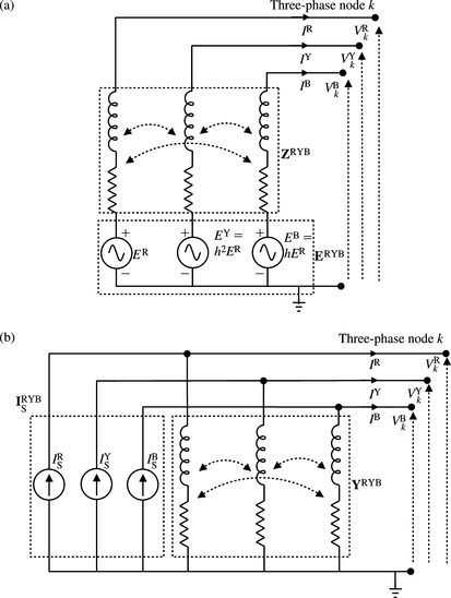
From Equation (6.68a), under a three-phase short-circuit fault at the machine terminals, the short-circuit current vector is given by ![]() . Substituting for ERYB from Equation (6.68a) we obtain
. Substituting for ERYB from Equation (6.68a) we obtain
Equation (6.70c) represents the machine’s three-phase Norton’s equivalent circuit model shown in Figure 6.27(b).
Induction machines
A three-phase induction machine model can be derived in a similar way to a synchronous machine model, with one exception. Viewed from its terminals, an induction machine appears as an open circuit in the ZPS network where the stator winding is connected in either delta or star with an isolated neutral as is usually the case. Thus, the machine’s ZPS impedance is infinite. Using the machine’s sequence admittances YP = 1/ZP, YN = 1/ZN and YZ = 0, as well as Equation (6.69a), the machine’s sequence admittance matrix is given by
 (6.71a)
Using Equation (6.68c), the induction machine phase admittance matrix is given by
 (6.71b)
In the case where YP ≈ YN, Equation (6.71b) reduces to
 (6.71c)
6.7.3 Three-phase analysis of ac current in the phase frame of reference
In Chapter 3, we presented three-phase lumped admittance matrix models of overhead lines and cables, and in Chapter 4, similar three-phase models were presented for transformers and other static power plant. Where ac short-circuit analysis is being undertaken, the prefault loadflow study that sets up the initial conditions for the short-circuit study may be based on a balanced or an unbalanced loadflow study. The latter study produces unbalanced voltages and currents in the network, whereas the former produces PPS voltages and currents only. Figure 6.28 illustrates a power system containing balanced three-phase voltage or current sources, an unbalanced power network such as an untransposed overhead line and a three-phase node k where a balanced or unbalanced short-circuit fault may occur.

Figure 6.28 Illustration of a three-phase network for multiphase short-circuit analysis in the phase frame of reference
Similar to the collection of lumped shunt elements, shown in Figure 6.17 for single-phase elements, the three-phase self-admittance matrix at any three-phase node can be calculated as the sum of all the individual element self-admittance matrices at that node. The three-phase admittance matrix of the entire system can then be constructed, and the three-phase system admittance matrix equation is given as
 (6.72a)
The elements of the three-phase admittance matrix of Equation (6.72a) are 3 × 3 matrices. Written in concise matrix form, Equation (6.72a) becomes
As described in Section 6.6, the matrix Y is sparse and generally symmetrical, and its inverse Z may be obtained by factorising Y into its upper triangle using Gaussian elimination and back substitution. Using the superposition theorem, the actual phase voltages at all nodes in the three-phase network are obtained using similar equations to those given in Equation (6.22), thus
The phase voltage changes ΔVRYB caused by the injected phase currents IRYB are given by
For a general shunt short-circuit fault of any type at node k, the injected phase currents at all nodes in the system except node k are zero. Thus,
From Equations (6.73), the actual phase voltages at the faulted node k are given by
Using the general phase fault impedance matrix of Equation (6.45b), the phase fault admittance matrix is given by
 (6.75)
The phase fault admittance matrix for various unbalanced faults through a fault impedance ZF and an earth impedance ZE can be calculated. For a single-phase to earth short-circuit fault, the phase fault admittance matrix is given by
 (6.76a)
For a two-phase unearthed fault, the phase fault admittance matrix is given by
 (6.76b)
For a two-phase to earth short-circuit fault, the phase fault admittance matrix is
 (6.76c)
For a three-phase earthed or unearthed short-circuit fault, the phase fault admittance matrix is given by
 (6.76d)
where m = 1 for a three-phase unearthed fault and m = 3 for a three-phase to earth fault as presented in Chapter 2.
Using the fault admittance matrix, the actual phase voltages at the faulted node k are
From Equations (6.74) and (6.77), we obtain the phase fault voltages as
where U is the identity matrix. Substituting Equation (6.78) in Equation (6.77) the phase fault currents at the faulted node k are given by
The actual phase voltages at any node throughout the network, say node i, are calculated using Equation (6.73), thus
The actual phase currents flowing in the network three-phase branches are given by
The phase current contributions of each machine, say the machine connected at node i, are calculated using Equation (6.70c) as follows:
Sequence currents and voltages, if required, can be calculated using the phase to sequence transformation ![]() and
and ![]()
6.7.4 Three-phase analysis and estimation of X/R ratio of fault current
General
Where the magnitude of the dc component of the short-circuit fault current is estimated from the X/R ratio at the fault location, the X/R ratio can be calculated using Thévenin’s impedance matrix at the fault location ![]() in accordance with IEC 60909 Method B, IEC 60909 Method C or IEEE C37.010 Method. These will be discussed in Chapter 7.
in accordance with IEC 60909 Method B, IEC 60909 Method C or IEEE C37.010 Method. These will be discussed in Chapter 7.
In general, the Thévenin’s phase impedance matrix ![]() representing the mutually coupled three-phase network is bilateral and the elements of
representing the mutually coupled three-phase network is bilateral and the elements of ![]() are reciprocal, i.e. ZRY = ZYR except in special cases. This may be due to the generally unequal PPS and NPS impedances of machines and the non-symmetric admittance matrices of quadrature boosters and phase shifting transformers.
are reciprocal, i.e. ZRY = ZYR except in special cases. This may be due to the generally unequal PPS and NPS impedances of machines and the non-symmetric admittance matrices of quadrature boosters and phase shifting transformers.
The effective X/R ratio at the fault location is dependent on the short-circuit fault type. To illustrate how the X/R ratio can be calculated, we use Figure 6.28 where the following equation can be written
 (6.83)
We will consider one-phase to earth and three-phase to earth short-circuit faults but the method is general and can be extended to cover other fault types.
One-phase to earth short-circuit fault
For a solid one-phase to earth short-circuit fault on phase R at node K, we have ![]() and
and ![]() Therefore, from the first row of Equation (6.83), we have
Therefore, from the first row of Equation (6.83), we have
Similar equations can be written where the faulted phase is either phase Y or phase B. Therefore, in general, the X/R ratio of the phase fault current is calculated from the self-impedance of the faulted phase, or
Alternatively, the X/R ratio can be calculated by transforming Equation (6.83) to the sequence reference frame using VPNZ = H−1VRYB, IPNZ = H−1IRYB and ![]() The result is given by
The result is given by
 (6.86)
As we discussed in Chapter 2, the boundary conditions IR = IF, IY = 0, IB = 0 and ![]() translate to
translate to ![]() and
and ![]() Using these sequence boundary conditions and Equation (6.86), the symmetrical component equivalent circuit is shown in Figure 6.29.
Using these sequence boundary conditions and Equation (6.86), the symmetrical component equivalent circuit is shown in Figure 6.29.

Figure 6.29 Calculation of X/R ratio of single-phase short-circuit fault current in an unbalanced three-phase network
Now, summing the three rows of Equation (6.86), or using Figure 6.29, and using ![]() , the following equation can be written
, the following equation can be written
Therefore, the equivalent X/R ratio of the phase fault current IR for a single-phase short-circuit fault on phase R is given by
 (6.88)
It is quite interesting to note that one third of the sum of the nine elements of the sequence impedance matrix for a one-phase fault on phase R is equal to the self-phase impedance of phase R that is Equations (6.84) and (6.87) are identical. Thus,
Equation (6.89) can be obtained using Equations (2.25) and (2.26a) from Chapter 2 even though Equation (2.26b) was derived assuming a bilateral network.
Three-phase to earth short-circuit fault
For a three-phase to earth short-circuit fault, we have ![]() However, unlike the balanced network analysis presented in Chapter 2, because the network is now unbalanced,
However, unlike the balanced network analysis presented in Chapter 2, because the network is now unbalanced, ![]() . Therefore from Equation (6.83) we have
. Therefore from Equation (6.83) we have
 (6.90)
 (6.91)
Therefore, using EY = h2ER, EB = hER and expanding Equation (6.91), the effective impedance seen by phase fault current R is given by
and the X/R ratio of phase R fault current is given by
 (6.92b)
The effective impedance seen by phase fault current Y is given by
and the X/R ratio of phase Y fault current is given by
 (6.93b)
The effective impedance seen by phase fault current B is given by
and the X/R ratio of phase B fault current is given by
 (6.94b)
It is important to note that the three-phase fault currents are generally unbalanced both in magnitude and phase and that the three X/R ratios are generally different. The differences being dependent on the degree of network unbalance.
In the author’s experience, and depending on the type of study being carried out, it is often more advantageous in three-phase unbalanced analysis to use actual physical units, i.e. volts, amps and ohms, instead of per-unit quantities.
6.7.5 Example
Example 6.4
The three-phase Thévenin’s impedance matrix at the fault location ![]() of Figure 6.28 is given by
of Figure 6.28 is given by

The balanced three-phase voltage sources have an rms value of unity. Calculate the fault currents and X/R ratios for a one-phase to earth fault on phase R, Y and B, and a three-phase to earth fault as presented in Section 6.7.4.
One-phase to earth fault
Using Equation (6.84), the current for a fault on phase R is equal to
Using Equation (6.85) and for a fault on phase R, we have
The sequence Thévenin’s impedance matrix at the fault location ![]() is calculated as
is calculated as
Using Equation (6.88), we have
Three-phase to earth fault
The Thévenin’s phase admittance matrix at the fault location ![]() is calculated as
is calculated as
Using Equation (6.91), we have
Using Equation (6.92a),
and the X/R ratio of phase R fault current is
Using Equation (6.93a),
and the X/R ratio of phase Y fault current is given by
Using Equation (6.94a),
and the X/R ratio of phase B fault current is given by
[1] ISBN 0701133380Grainger J., Stevenson W.D. Power System Analysis. 1994.
[2] Elgerd O.I. Electric Energy Systems Theory. McGraw-Hill Int. Ed.; 1983. 0-07-66273-8
[3] Anderson P.M. Analysis of Faulted Power Systems. Ames, IA: Iowa State Press; 1973.
[4] Nor K.M., et al. Improved three-phase power-flow methods using sequence components. IEEE Transactions on Power Systems. August 2005;Vol. 20(No. 3):1389-1397.
[5] Berman A., et al. Analysis of faulted power systems by phase coordinates. IEEE Transactions on Power Delivery. April 1998;Vol. 13(No. 2):587-595.