
1 Introduction to power system faults
1.1 General
In this introductory chapter, we introduce the important terminology of fault current waveform, discuss the need for power system fault analysis and the effects of fault currents in power systems. Per-unit analysis concept of single-phase and three-phase power systems is presented including the base and per-unit equations of self and mutual impedances and admittances.
1.2 Structure of power systems
Electrical ac power systems consist of three-phase generation systems, transmission and distribution networks, and loads. The networks supply large three-phase industrial loads at various distribution and transmission voltages as well as single-phase residential and commercial loads. In some countries, e.g. North America, the term subtransmission is used to denote networks with voltage classes between transmission and distribution. Distribution voltages are typically 10–60 kV, subtransmission voltages are typically 66–138 kV and transmission voltages are typically above 138 kV. Generated voltages are up to 35 kV for generators used in large electrical power stations. Power station auxiliary supply systems and industrial power systems supply a significant amount of induction motor load. Residential and commercial loads include a significant amount of single-phase induction motor loads.
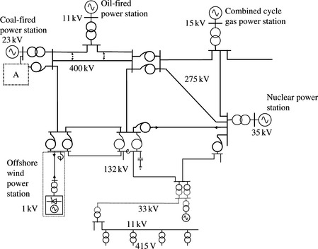
For over a century, electric power systems used synchronous machines for the generation of electricity. However, in the twenty-first century, the generation of electricity from renewable energy sources such as wind has begun to expand at a large pace. Generally, such generation systems use a variety of asynchronous machines as well as machines interfaced to the three-phase network through a low voltage direct current link or a power electronics converter. Typical ratings of wind turbine generators are currently up to 5 MW and typical generated voltage range from 0.4 to 5 kV. The mix of synchronous, asynchronous and converter isolated electrical generation systems is expected to change the behaviour of three-phase power systems following disturbances such as short-circuit faults. Figure 1.1 illustrates a typical structure and components of a generation, transmission and distribution power system and Figure 1.2 illustrates a typical auxiliary electrical supply system for a large power station representing box A in Figure 1.1.

1.3 Need for power system fault analysis
1.3.1 General
Short-circuit analysis is carried out in electrical power utility systems, industrial power systems, commercial power systems and power station auxiliary systems. Other special applications are in concentrated power system installations on board military and commercial ships and aircraft. Short-circuit calculations are generally performed for a number of reasons. These are briefly described in the next sections.
1.3.2 Health and safety considerations
Short-circuit fault analysis is carried out to ensure the safety of workers as well as the general public. Power system equipment such as circuit-breakers can fail catastrophically if they are subjected to fault duties that exceed their rating. Other equipment such as busbars, transformers and cables can fail thermally or mechanically if subjected to fault currents in excess of ratings. In addition, to ensure safety, short-circuit fault analysis is carried out and used in the calculation of rise of earth potential at substations and overhead line towers. Other areas where fault analysis is carried out are for the calculation of induced voltages on adjacent communication circuits, pipelines, fences and other metallic objects.
1.3.3 Design, operation and protection of power systems
Short-circuit current calculations are made at the system design stage to determine the short-circuit ratings of new switchgear and substation infrastructure equipment to be procured and installed. System reinforcements may be triggered by network expansion and/or the connection of new generating plant to the power system. Routine calculations are also made to check the continued adequacy of existing equipment as system operating configurations are modified. In addition, calculations of minimum short-circuit currents are made and these are used in the calculation of protection relay settings to ensure accurate and coordinated relay operations. In transmission systems, short-circuit currents must be quickly cleared to avoid loss of synchronism of generation plant and major power system blackouts. Maximum short-circuit current calculations are carried out for the design of substation earth electrode systems. Short-circuit analysis is also carried out as part of initial power quality assessments for the connection of disturbing loads to electrical power networks. These assessments include voltage flicker, harmonic analysis and voltage unbalance. Other areas where short-circuit analysis is carried out is in the modification of an existing system or at the design stage of new electrical power installations such as a new offshore oil platform, new petrochemical process plant or the auxiliary electrical power system of a new power station. The aim is to determine the short-circuit rating of new switchgear and other substation infrastructure equipment that will be procured and installed.
1.3.4 Design of power system equipment
Switchgear manufacturers design their circuit-breakers to ensure that they are capable of making, breaking and carrying, for a short time, the specified short-circuit current. Equipment with standardised short-circuit ratings are designed and produced by manufacturers. Also, manufacturers of substation infrastructure equipment and other power system plant, e.g. transformers and cables, use the short-circuit current ratings specified by their customers to ensure that the equipment is designed to safely withstand the passage of these currents for the duration specified.
1.4 Characteristics of power system faults
1.4.1 Nature of faults
A fault on a power system is an abnormal condition that involves an electrical failure of power system equipment operating at one of the primary voltages within the system. Generally, two types of failure can occur. The first is an insulation failure that results in a short-circuit fault and can occur as a result of overstressing and degradation of the insulation over time or due to a sudden overvoltage condition. The second is a failure that results in a cessation of current flow or an open-circuit fault.
1.4.2 Types of faults
Short-circuit faults can occur between phases, or between phases and earth, or both. Short circuits may be one-phase to earth, phase to phase, two-phase to earth, three-phase clear of earth and three-phase to earth. The three-phase fault that symmetrically affects the three phases of a three-phase circuit is the only balanced fault whereas all the other faults are unbalanced. Simultaneous faults are a combination of two or more faults that occur at the same time. They may be of the same or different types and may occur at the same or at different locations. A broken overhead line conductor that falls to earth is a simultaneous one-phase open-circuit and one-phase short-circuit fault at one location. A short-circuit fault occurring at the same time on each circuit of a double-circuit overhead line, where the two circuits are strung on the same tower, is a simultaneous fault condition. A one-phase to earth short-circuit fault in a high impedance earthed distribution system may cause a sufficient voltage rise on a healthy phase elsewhere in the system that a flashover and short-circuit fault occurs. This is known as a cross-country fault. Most faults do not change in type during the fault period but some faults do change and evolve from say a one-phase to earth short circuit to engulf a second phase where it changes to a two-phase to earth short circuit fault. This can occur on overhead lines or in substations where the flashover arc of the faulted phase spreads to other healthy phases. Internal short circuits to earth and open-circuit faults can also occur on windings of transformers, reactors and machines as well as faults between a number of winding turns of the same phase.
1.4.3 Causes of faults
Open-circuit faults may be caused by the failure of joints on cables or overhead lines or the failure of all the three phases of a circuit-breaker or disconnector to open or close. For example, two phases of a circuit-breaker may close and latch but not the third phase or two phases may properly open but the third remains stuck in the closed position. Except on mainly underground systems, the vast majority of short-circuit faults are weather related followed by equipment failure. The weather factors that usually cause short-circuit faults are: lightning strikes, accumulation of snow or ice, heavy rain, strong winds or gales, salt pollution depositing on insulators on overhead lines and in substations, floods and fires adjacent to electrical equipment, e.g. beneath overhead lines. Vandalism may also be a cause of short-circuit faults as well as contact with or breach of minimum clearances between overhead lines and trees due to current overload.
Lightning strikes may discharge currents in the range of a few kiloamps up to 100 or 200 kA for a duration of several microseconds. If the strike hits an overhead line or its earth wire, the voltage produced across the insulator may be so large that a back-flashover and short circuit occurs. This may involve one or all three phases of a three-phase electrical circuit and as a result a transient power frequency short-circuit current flows. For example, consider a 132 kV overhead three-phase transmission line of steel tower construction and one earth wire. The surge impedances of the tower, line phase conductors and earth wire are given as 220, 350 and 400 ω, respectively, and the tower’s earthing or footing resistance is 50 ω. The line’s rated lightning impulse withstand voltage to earth is 650 kV peak phase to earth (nominal peak phase to earth voltage is (132 kV × ![]() = 107.8 kV). A lightning strike with a reasonably modest peak current of 10 kA hits a tower on the line. The voltage produced across the line’s insulator is approximately equal to 10 kA × 105 ω = 1050 kV This significantly exceeds the line’s insulation strength causing back-flashover on all three phases of the line and a three-phase to earth short-circuit fault. If the shielding of the earth wire fails and the lightning strike hits one of the phase conductors near a tower, then the voltage produced across the line’s insulator is approximately equal to 10 kA × 175 ω = 1750 kV. In this case, a smaller lightning current in the order of 3.8 kA would be sufficient to cause a back-flashover and hence a short-circuit fault. On lower voltage distribution lines, even ‘indirect’ lightning strikes, i.e. those that hit nearby objects to the line may produce a sufficiently large voltage on the line to cause an insulator flashover and a short-circuit fault. Other causes of short-circuit faults are fires. The smoke of fires beneath overhead lines consists of small particles which encourage the breakdown of the air that is subjected to the intense electric field of a high voltage power line. The hot air in the flames of a fire has a much lower insulation strength than air at ambient temperature. A flashover across an insulator to earth or from a phase conductor to a tree may occur.
= 107.8 kV). A lightning strike with a reasonably modest peak current of 10 kA hits a tower on the line. The voltage produced across the line’s insulator is approximately equal to 10 kA × 105 ω = 1050 kV This significantly exceeds the line’s insulation strength causing back-flashover on all three phases of the line and a three-phase to earth short-circuit fault. If the shielding of the earth wire fails and the lightning strike hits one of the phase conductors near a tower, then the voltage produced across the line’s insulator is approximately equal to 10 kA × 175 ω = 1750 kV. In this case, a smaller lightning current in the order of 3.8 kA would be sufficient to cause a back-flashover and hence a short-circuit fault. On lower voltage distribution lines, even ‘indirect’ lightning strikes, i.e. those that hit nearby objects to the line may produce a sufficiently large voltage on the line to cause an insulator flashover and a short-circuit fault. Other causes of short-circuit faults are fires. The smoke of fires beneath overhead lines consists of small particles which encourage the breakdown of the air that is subjected to the intense electric field of a high voltage power line. The hot air in the flames of a fire has a much lower insulation strength than air at ambient temperature. A flashover across an insulator to earth or from a phase conductor to a tree may occur.
Equipment failure, e.g. machines, transformers, reactors, cables, etc., cause many short-circuit faults. These may be caused by failure of internal insulation due to ageing and degradation, breakdown due to high switching or lightning over-voltages, by mechanical incidents or by inappropriate installation. An example is a breakdown of a cable’s polymer insulation due to ageing or to the creation of voids within the insulation caused by an external mechanical force being accidentally applied on the cable.
Short-circuit faults may also be caused by human error. A classical example is one where maintenance staffs inadvertently leave isolated equipment connected through safety earth clamps when maintenance work is completed. A three-phase to earth short-circuit fault occurs when the equipment is reenergised to return it to service.
On mainly overhead line systems, the majority of short-circuit faults, typically 80–90%, tend to occur on overhead lines and the rest on substation equipment and busbars combined. Typically, on a high voltage transmission system with overhead line steel tower construction, such as the England and Wales transmission system, long-term average short-circuit fault statistics show that around 300 short-circuit faults occur per annum. Of these, 67% are one-phase to earth, 25% are phase to phase, 5% are three-phase to earth and three-phase clear of earth, and 3% are two-phase to earth. About 77% of one-phase to earth faults are caused by lightning strikes followed by wind and gales then salt pollution on insulators. Although lightning can cause some phase-to-phase faults, by far the most common causes of these faults are snow/ice followed by wind/gales that cause two line conductors to clash. The majority of three-phase to earth and two-phase to earth faults in England and Wales are caused by lightning then wind and gales. On wood-pole overhead lines, e.g. some 132 kV and lower in England and Wales, between 50% and 67% of short-circuit faults are two-phase and three-phase faults.
1.4.4 Characterisation of faults
Because they are unbalanced, one-phase open-circuit and two-phase open-circuit faults are characterised by the negative and zero phase sequence voltages and currents they generate at the fault location and elsewhere in the power system particularly at substations where electrical machines are connected. Machines are vulnerable to damage by overheating due to excessive negative phase sequence currents flowing into them. Short-circuit faults are characterised by the short-circuit current and its components. These are the ac or symmetrical root mean square (rms) short-circuit current, dc short-circuit current or dc time constant or X/R ratio, and the overall asymmetrical short-circuit current. These are described in the next section.
To characterise the short-circuit infeed from one short-circuit source, a group of such sources or an entire system, the concept of short-circuit fault level is useful:
where Irms(kA) is the rms short-circuit current infeed at the point of fault and VPhase-Phase(kv) is the prefault phase-to-phase voltage at the point of fault. For example, for an rms short-circuit current of 54 kA and a 404 kV prefault voltage in a 400 kV system, the short-circuit fault level is equal to 37.786 GVA. The system short-circuit fault level or infeed gives a measure of the strength or weakness of the system at the point of fault. For a given system short-circuit fault level or MVAInfeed at a busbar, the equivalent system impedance seen at the busbar in per unit on MVABase and phase-to-phase ![]() is given by
is given by
 (1.2)
(1.2)where the definition of base quantities is presented in Section 1.7. Where the prefault and base voltages are equal, we have
High system strength is characterised by a high short-circuit fault level infeed and thus low system impedance, and vice versa. ZS is also equal to the Thévenin’s impedance.
Sometimes, an MVA figure is used to describe the short-circuit rating of a circuit-breaker in MVA. This practice is discouraged as it can easily lead to confusion and errors. For example, consider a 5000 MVA, 132 kV circuit-breaker that is to be used in a 110 kV system. The 5000 MVA rating becomes a meaningless and the correct figure should be
Another important characteristic of a short-circuit fault in the case of earth faults is its fault impedance. In general, in the event of a flashover, the fault impedance consists of the flashover arc resistance and the earthing impedance of the object to which the flashover occurs. For example, where this object is an overhead line’s steel tower, the earthing impedance is that of the tower footing resistance in parallel with the line’s earth wire impedance, where it exists (this is discussed in detail in Chapter 10). The fault impedance is generally neglected in higher voltage systems when calculating maximum short-circuit currents to obtain conservative results. However, earthing impedances are taken into account when calculating rise of earth potential for short-circuit faults in substations and on overhead lines’ towers. In lower voltage distribution systems, many short-circuit faults occur due to a flashover from a line to a tree which may present a significant earthing impedance depending on earth resistivity. The resistance of the flashover arc can be estimated using the following empirical formula:
where ![]() is the length of the arc in m in still air and lrms is the rms short-circuit current in kA. For example, for
is the length of the arc in m in still air and lrms is the rms short-circuit current in kA. For example, for ![]() = 7.75 m on a typical 400 kV overhead line and Irms = 30 kA, we obtain RArc = 0.12 ω.
= 7.75 m on a typical 400 kV overhead line and Irms = 30 kA, we obtain RArc = 0.12 ω.
1.5 Terminology of short-circuit current waveform and current interruption
In order to calculate short-circuit current duties on power system equipment, it is important to define the terminology used in characterising the short-circuit current waveform. Figure 1.3 shows a simple balanced three-phase electric circuit where L and R are the circuit inductance and resistance for each phase, and Le and Re are the earth return path inductance and resistance, respectively.

The balanced three-phase voltage sources are given by
where Vrms is rms voltage magnitude, ω = 2πf in rad/s, f is power frequency in Hz and ϕi is voltage phase angle in rad given by
If a solid three-phase to earth connection or short-circuit fault is made simultaneously between phases r, y, b and earth e at t = 0, we can write
Substituting i = r, y, b in Equation (1.7) and adding the three equations, we obtain
 (1.8)
(1.8)Since the three-phase voltage sources are balanced we have
Also, from Figure 1.3, we have
Therefore, substituting Equations (1.9) and (1.10) into Equation (1.8), we obtain
The solution of Equation (1.11) is given by
 (1.12)
where K is a constant that satisfies the initial conditions. Since the three-phase system is symmetrical and balanced, ie(t = 0) = 0. Thus, Equation (1.12) gives K = 0 and ie(t) = 0. That is, following a simultaneous three-phase short circuit, no current will flow in the earth return connection and the three fault currents ii(t) will flow independently as in single-phase circuits. Therefore, with ie(t) = 0, the solution of Equation (1.7) is given by
 (1.13)
Equation (1.13) can be written as the sum of an ac component and a unidirectional dc component as follows:
where
and
In this analysis, the magnitude of the ac current component is constant because we assumed that the source inductance L is constant or time independent. This assumption is only generally valid if the location of short-circuit fault is electrically remote from electrical machines feeding short-circuit current into the fault. This aspect is discussed in detail later in this book where practical time-dependent source inductance is considered. The initial magnitude of the dc current component in any phase depends on the instant on the voltage waveform when the short circuit occurs, i.e. on ϕr and on the magnitude of the ac current component Irms. The rate of decay of the dc current component in the three phases depends on the circuit time constant L/R or circuit X/R ratio where X/R = ωL/R. Again, the assumption of a constant L results in a time-independent X/R ratio or constant rate of decay.
Short-circuit currents are detected by protection relays which initiate the interruption of these currents by circuit-breakers. Figure 1.4 shows a general asymmetrical short-circuit current waveform and the terminology used to describe the various current components as well as the short-circuit current interruption.

Figure 1.4 (a) Asymmetrical short-circuit current waveform and current interruption and (b) modern 420 kV SF6 circuit breaker
From Figure 1.4, the following quantities and terms are defined:
tF = Instant of short-circuit fault.
tA = Instant of ‘initial peak’ of short-circuit current.
t1 = Instant of energisation of circuit-breaker trip circuit.
Δt2 = Circuit-breaker opening time.
t2 = Instant of circuit-breaker contact separation = instant of arc initiation.
Δt3 = Circuit-breaker current arcing time.
t3 = Instant of final arc extinction = instant of short-circuit current interruption.
tB = Instant of peak of major current loop just before current interruption.
![]() Theoretical current at the instant of short-circuit fault tF where
Theoretical current at the instant of short-circuit fault tF where ![]() is the rms short-circuit current at t = tF.
is the rms short-circuit current at t = tF.
AA″ = ‘Initial peak’ short-circuit current at t = tA and is denoted ip. ip is also termed ‘1/2 cycle peak’ current, ‘peak make’ current or ‘making’ current. AA″ = AA″ + A′A″ where AA′ = magnitude of dc current component at t = tA and A′A″ = peak ac current component at t = tA and is equal to ![]() × rms current at t = tA.
× rms current at t = tA.
BB′ = Peak short-circuit current at t = tB and is denoted ib. BB″ = BB′ + B′B″ where BB′ = magnitude of dc current component at t = tB and B′B″ = peak ac current component at t = tB and is equal to ![]() × Ib, where Ib is rms current at t = tB.
× Ib, where Ib is rms current at t = tB.
Percentage dc current component at t = tB given by (BB′ × 100)/B′B″.
A1 + A2 = Area that corresponds to the arc energy measured from instant of contact separation or arc initiation t2 to instant of final arc extinction or current interruption t3.
1.6 Effects of short-circuit currents on equipment
1.6.1 Thermal effects
Short-circuit currents flowing through the conductors of various power system equipment create thermal effects on conductors and equipment due to heating and excess energy input over time as measured by I2T where I is the short-circuit current magnitude and T is the short-circuit current duration. Because the short-circuit duration, including short circuits cleared by protection in back-up clearance times, is quite short, the heat loss from conductors during the short circuit is usually very low. Generally, both ac and dc components of the short-circuit current contribute to the thermal heating of conductors. Extreme values of the time constant of the dc short-circuit current component may be up to 150 ms so that by 500 ms from the instant of short circuit, the dc component is nearly vanished and nearly all its generated heat will have dissipated by around 1 s. For the ac current component, the heat dissipation depends on the ratio of the initial subtransient rms current to steady state rms current. For a typical ratio of about 2.5, the amount of conductor heat dissipation will be around 50% at 1 s and nearly 65% at 3 s. The three-phase short-circuit fault normally gives rise to the highest thermal effect on equipment. For cables of larger conductor sizes, the thermal limit is usually imposed by the sheath/armour as opposed to the core conductor under short-circuit earth fault conditions. During the making of high short-circuit currents by inadequately rated circuit-breakers, their contacts may weld together encouraged by a prestriking flashover arc and possibly contact popping.
1.6.2 Mechanical effects
Short-circuit currents flowing through the conductors of various power system equipment create electromagnetic forces and mechanical stresses on equipment such as overhead line conductors, busbars and their supports, cables and transformer windings. Mechanical forces on transformer windings are both radial and axial. The radial force is a repulsion force between the inner and outer windings and tends to crush the inner winding towards the transformer core and burst the outer winding outwards. The axial force tends to displace the windings, or part of the winding, with respect to each other. The transformer windings must be designed to withstand the mechanical forces created by the short-circuit currents. The electromagnetic forces produced by short-circuit currents in three-core unarmoured cables tend to repel the cores from each other and could burst the cable altogether leading to insulation damage if the cores are not adequately bound.
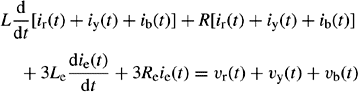
The electromagnetic forces acting on two parallel, round conductors carrying currents i1 and i2, as shown in Figure 1.5, are given by

 (1.18)
where d is the distance between the centres of the conductors in m and l is the conductor length between supports in m. μo = 4π10−7 H/m is the permeability of vacuum. Since i1(t) and i2(t) are instantaneous currents in amps as given in Equation (1.13), the electromagnetic force F(t) is clearly time dependent. In the general case, F(t) will contain a dc component, a power frequency component and a double-power frequency component, i.e. a 100 Hz component in a 50 Hz system. In practical installations, l » d and d » a where a is the conductor diameter in m. Therefore, Equation (1.18) reduces to
Where the currents flow in the two conductors in the same direction, the forces are compressive, i.e. pulling the conductors together but if the currents are flowing in opposite directions, the forces would repel the conductors away from each other. This is illustrated in Figure 1.5. To illustrate how this equation may be used, consider an overhead line with a twin conductor bundle per phase (overhead lines are discussed in detail in Chapter 3) and d = 0.5 m. The short-circuit current satisfies Equation (1.13) and has an rms value of 20 kA per phase and an X/R ratio equal to 15. The maximum attraction forces on each conductor per metre produced by the first peak of the asymmetrical short-circuit current are to be calculated. Individual conductor rms current is 20/2 =10 kA. Using Equation (1.13), the maximum value of the initial peak current is calculated assuming maximum dc current offset which corresponds to a short-circuit fault that occurs at a voltage phase angle ![]() . Therefore, using Equation (1.13), the initial peak current is equal to
. Therefore, using Equation (1.13), the initial peak current is equal to
The attraction forces on each conductor are calculated as
The electromagnetic forces acting on three rigid, parallel and round conductors, shown in Figure 1.6, under a balanced three-phase short-circuit fault condition can be calculated approximately using the following equations:
In Equations (1.20)-(1.22), ir(t), iy(t) and ib(t) are the instantaneous currents given in Equation (1.13) in amps. Substituting these currents into Equations (1.20)-(1.22), it can be shown that the maximum force occurs on the middle conductor and is given by
where ip is the initial peak short-circuit current that corresponds to AA″ in Figure 1.4. During a phase-to-phase short-circuit fault, it can be shown that the maximum electromagnetic force between the two faulted conductors is given by
where ip is the initial peak short-circuit current.
Where the conductors are not round, e.g. rectangular, d in all the electromagnetic force equations is replaced by an effective distance deff equal to the effective geometric mean distance between the rectangular conductors.
1.7 Per-unit analysis of power systems
1.7.1 General
Steady state network analysis on initially balanced three-phase networks generally employ complex phasors and involve the calculation of active and reactive power flows, voltages and currents in the network. Usually, such calculations are carried out using per-unit values of actual physical quantities such as voltages, currents or impedances. The advantages of per-unit systems of analysis are generally covered in most introductory power systems textbooks and will not be repeated. However, as we will discuss later in this book, the use of actual physical units such as volts, amps, ohms and Siemens is more advantageous in multiphase network analysis.
1.7.2 Single-phase systems
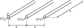
The per-unit system of analysis is based on the application of Ohm’s law to a single impedance or admittance as illustrated in Figure 1.7(a).
Figure 1.7 Per-unit analysis of (a) single-phase impedance and admittance and (b) three-phase connections
Using actual physical units of kilovolts, kiloamps, ohms and Siemens, the voltage drop across the impedance and injected current into the admittance are given by
where V, I, Z and Y are complex phasors representing actual physical quantities of voltage, current, impedance and admittance, respectively. To calculate a per-unit value for each of these quantities, a corresponding base quantity must be defined first. Let VBase,kV and IBase,kA be the base voltage and base current, respectively. Therefore, Equations (1.25a) and (1.25b) can be written as follows:
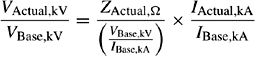
and

or
and
where
By defining VBase,kV and IBase,kA, ZBase,ω and YBase,S are also defined as shown in Equations (1.28) and (1.29), and the per-unit values of the actual voltage and current are also defined in Equation (1.27). It should be noted that the base quantities VBase,kV and IBase,kA are defined as real numbers so that the phase angles of Vpu and Ipu remain unchanged from VActual,kV and IActual,kA, respectively. Using Equation (1.27), we have
or
or
where
We note that by defining VBase,kV and IBase,kA, MVABase is also defined according to Equation (1.30b). In practical power system analysis, it is more convenient to define or choose MVABase and VBase,kV and calculate IBase,kV if required. Therefore, using Equations (1.27) and (1.30b), we have
 (1.31)
Also, using Equations (1.28) and (1.30b), we can write

and
or using Equation (1.30b), we have
 (1.32)
Substituting Equation (1.32) in Equations (1.28) and (1.29), we obtain
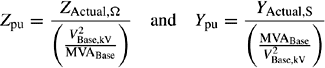 (1.33)
To convert per-unit values to per cent, the per-unit values are multiplied by 100.
1.7.3 Change of base quantities
The per-unit values that are calculated by generator manufacturers and sometimes transformer manufacturers are usually based on the rated voltage and rated apparent power of the equipment. However, transmission and distribution system analysis using per-unit values are based on a single MVA base of typically 100 MVA. In industrial power systems and power station auxiliary supply systems, 10 MVA base is generally found more convenient. For transformers, it is almost always the case that the rated voltage of at least one of the windings is not equal to the base voltage of the network to which the winding is connected. This is discussed in detail in Chapter 4. To determine how, in general, per-unit values are calculated using new base quantities, let the two base quantities be MVABase-1, VBase-1,kV and MVABase-2, VBase-2,kV, and it is required to convert from Base-1 to the new Base-2. Using Equation (1.27), we can write
giving
Using Equation (1.31), we have

giving
or using Equation (1.30b), we have
From Equation (1.33), we have

or
 (1.36)
and similarly for the per-unit admittance
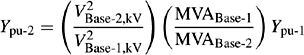 (1.37)
1.7.4 Three-phase systems
The above analysis of single-phase systems can be easily extended to three-phase systems or equipment using the following basic relations that apply irrespective of whether the equipment is star or delta connected
and
where MVA3-Phase is three-phase base apparent power, MVA1-Phase is one-phase base apparent power, VPhase-Phase,kV is phase-to-phase base voltage and ILine,kA is base line current. The relationships between base voltages and base currents for star- and delta-connected three-phase equipment is shown in Figure 1.7(b):
where VPhase,kV and IPhase,kA correspond to the base voltage and current quantities as used in Section 1.7.2 for a single-phase system. Using Equations (1.38) and (1.40) in Equations (1.31), (1.33), (1.34), (1.35b), (1.36) and (1.37), we obtain
 (1.42)
 (1.43)
 (1.45)
 (1.46)
1.7.5 Mutually coupled systems having different operating voltages
In many electrical power systems, double-circuit overhead lines are used for the transport of bulk power. The modelling of these lines is presented in detail in Chapter 3. For now, we state that these lines consist of two three-phase circuits strung on the same tower. In this section, we present the general case of the derivation of the per-unit values of the mutual impedance and mutual susceptance of two mutually coupled circuits operating at different voltages. The analysis is general and applies also to mutually coupled cable circuits and mutually coupled transformer windings.
Base and per-unit values of mutual inductive impedance
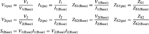
Figure 1.8 shows two mutually coupled inductive circuits having different design and operating voltages. The series voltage drop across each circuit is given by

Figure 1.8 Per-unit analysis of two mutually coupled inductive circuits having different design and operating voltages
where V is in volts, I is in amps, ZS1 and ZS2 are the self-impedances of circuits 1 and 2, respectively, in ohms, and ZM is the mutual impedance between the two circuits in ohms. Using the same base apparent power for both circuits, let the base quantities of circuits 1 and 2 be defined as follows:
 (1.48)
We note that for now, we have not yet defined the base or per-unit values for ZM. Using Equation (1.48) and substituting the actual quantities, e.g. V1 = V1(pu) × V1(Base), into Equation (1.47), we obtain
and
Dividing Equation (1.49a) by V1(Base) and Equation (1.49b) by V2(Base), we obtain
and
or
From Equations (1.50) and (1.51), the per-unit value of ZM is defined as
 (1.52a)
And the base impedance of ZM is defined as
From Equation (1.48), S(Base) = V1(Base)I1(Base) = V2(Base)I2(Base) or
Substituting Equation (1.53) into Equation (1.52b), and using S(Base) in MVA, V1(Base) and V2(Base) in kV, we obtain
Substituting Equation (1.54) into Equation (1.52a), we have
 (1.55)
In the above equations, if the voltages are phase to earth then the apparent power is single-phase power but if the voltages used are phase to phase, then the apparent power to be used is the three-phase value.
An equivalent alternative approach is to define a per-unit mutual impedance on the base of each circuit as follows:
 (1.56)
Now
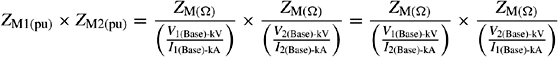
and using Equation (1.52b), we obtain ZM1(pu) × ZM2(pu) = ZM(pu)ZM(pu) = ZM2M(pu) or
Equations (1.55) and (1.57) are identical.
Base and per-unit values of mutual capacitive admittance
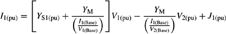
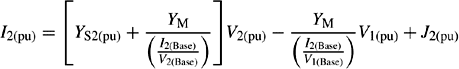
Figure 1.9 shows two mutually coupled capacitive circuits having different design and operating voltages. Using self and mutual admittance terms to maintain generality, the injected current into each circuit at one end of the circuit is given by

Figure 1.9 Per-unit analysis of two mutually coupled capacitive circuits having different design and operating voltages
where V is in volts, I is in amps, YS1 and YS2 are the self-admittances of circuits 1 and 2 in Siemens, respectively, and YM is the mutual admittance between the two circuits in Siemens. Using the same base apparent power for both circuits, let the base quantities of circuits 1 and 2 be defined as follows:
 (1.59)
We note that for now, we have not yet defined the base or per-unit values for YM. Using Equation (1.59) in Equation (1.58), we obtain
and
 (1.60b)
Dividing Equation (1.60a) by I1(Base) and Equation (1.60b) by I2(Base), we obtain
 (1.61a)
and
 (1.61b)
or
and
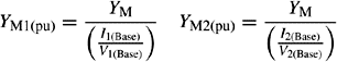
where
 (1.63a)
and the base admittance of YM is given by
Also
 (1.64)
Using SBase = V1(Base)I1(Base) = V2(Base)I2(Base) in Equation (1.63b), S(Base) in MVA, V1(Base) and V2(Base) in kV, we obtain
Substituting Equation (1.65) in Equation (1.63a), we obtain
 (1.66)
In the above equations, if the voltages are phase to earth then the apparent power is single-phase power but if the voltages used are phase to phase, then the apparent power to be used is the three-phase value. From Equation (1.64), we have

or
For practical overhead line analysis at power frequency, e.g. 50 or 60 Hz, YM(pu) = jBM(pu), YM1(pu) = jBM1(pu) and YM2(pu) = jBM2(pu) where B is shunt susceptance. Therefore, Equation (1.67) reduces to
1.7.6 Examples
Example 1.1
Figure 1.10 shows two inductively coupled circuits having operating (and design) voltages of 275 and 400 kV phase to phase, carrying currents of 1 and 2 kA, and have actual voltage magnitudes at end A of 270 and 406 kV, respectively. The self and mutual impedances of the circuits are shown on the figure. Calculate all quantities shown on the figure in per unit using a 100 MVA base, 275 and 400 kV base voltages for the circuits. In addition, calculate the induced voltages in each circuit in actual and in per-unit values.

Figure 1.10 Two inductively coupled circuits having different operating (and design) voltages for use in Example 1.1
The per-unit voltages at end A are 270 kV/275 kV = 0.9818 pu and 406 kV/400 kV = 1.015 pu. Circuit 1 base current is 100 MVA/![]() and circuit 1 current in per unit is 1 kA/0.21 kA = 4.76 pu. Circuit 2 base current is 100 MVA/(
and circuit 1 current in per unit is 1 kA/0.21 kA = 4.76 pu. Circuit 2 base current is 100 MVA/(![]() × 400 kV) = 0.1443 kA and circuit 2 current in per unit is 2 kA/0.1443 kA = 13.86 pu.
× 400 kV) = 0.1443 kA and circuit 2 current in per unit is 2 kA/0.1443 kA = 13.86 pu.
Base impedance of circuit 1 is (275 kV)2/100 MVA = 756.25 ω. Per-unit value of circuit 1 self-impedance is (6 + j30)ω/756.25 ω = (0.00793 + j0.0396)pu or (0.793 + j3.96)%.
Base impedance of circuit 2 is (400 kV)2/100 MVA = 1600 ω. Per-unit value of circuit 2 self-impedance is (3.5 + j25)ω/1600 ω = (0. 0022 + j0.0156)pu or (0.22 + j1.56)%.
Base impedance of mutual impedance is (400 kV × 275 kV)/100 MVA = 1100 ω and per-unit value of mutual impedance is (2.5 + j10)ω/1100 ω = (0.00227 + j0.00909)pu or (0.227 + j0.909)%. Alternatively,
and
Induced voltage in circuit 2 due to current in circuit 1 is (2.5 + j10)ω × 1 kA = (2.5 + j10)kV or in per unit (2.5 + j10)kV/(400kV/![]() ) = (0.0108 + j0.0433)pu. Alternatively, it can be calculated as (0.00227 + j0.00909)pu × 4.76 pu = (0.0108 + j0.0433)pu. The induced per-unit voltage in circuit 1 due to circuit 2 current can be similarly calculated.
) = (0.0108 + j0.0433)pu. Alternatively, it can be calculated as (0.00227 + j0.00909)pu × 4.76 pu = (0.0108 + j0.0433)pu. The induced per-unit voltage in circuit 1 due to circuit 2 current can be similarly calculated.
Example 1.2
Figure 1.11 shows two 400 and 275 kV capacitively coupled circuits. The actual voltages at end A, the self susceptance of each circuit and the mutual susceptance between the two circuits are shown on the figure. Calculate all quantities shown on the figure in per-unit using a 100 MVA base. In addition, calculate the charging current of each circuit at end A including the current flowing through the mutual susceptance. All calculations are to be carried out in physical units and in per-unit.

Figure 1.11 Two capacitively coupled circuits having different operating (and design) voltages for use in Example 1.2
The per-unit voltages at end A are 283 kV/275 kV = 1.029 pu and 404 kV/400 kV = 1.01 pu. Circuit 1 base current is 0.21 kA and circuit 2 base current is 0.1443 kA.
Base admittance of circuit 1 is 100 MVA/(275 kV)2 = 0.00132 S and per-unit value of self-susceptance is j150 × 10−6 S/0.00132 S = j0.1136 pu or j11.36%. Base admittance of circuit 2 is 100 MVA/(400 kV)2 = 6.25 × 10⁻⁴ S and per-unit value of self-susceptance is j200 × 10−6 S/(6.25 × 10−4 S) = j0.32 pu or j32%.
Base value of mutual susceptance is 100 MVA/(400 kV × 275 kV) = 9.09 × 10⁻⁴ S and per-unit value of mutual susceptance is j40 × 10−6 S/(9.09 × 10−4 S) = j0.044 pu or j4.4%. Alternatively,
and
thus YM(pu) = ![]() = j0.044 pu or j4.4%.
= j0.044 pu or j4.4%.
Circuit 1 charging current due to self susceptance is equal to j150 × 10−6 S × (283 × 103V/![]() ) = j24.51 A or j24.51 A/210 A = j0.1167 pu. Similarly, circuit 2 charging current due to self susceptance is equal to j46.65 A or j46.65 A/144.3 A = j0.3230 pu.
) = j24.51 A or j24.51 A/210 A = j0.1167 pu. Similarly, circuit 2 charging current due to self susceptance is equal to j46.65 A or j46.65 A/144.3 A = j0.3230 pu.
Current flowing through the mutual susceptance is equal to j40 × 10−6 S × (404 × 103 — 283 × 103)V/![]() = j2.79 A.
= j2.79 A.
Charging current of circuit 1 is equal to j24.51 A - j2.79 A = j21.72 A or j21.72 A/210 A = j0.103 pu.
Charging current of circuit 2 is equal to j46.65 A + j2.79 A = j49.44 A or j49.44 A/144.3 A = j0.3426 pu.