2.2.1 Balanced three-phase voltage and current phasors

Mathematically, balanced three-phase voltages (or currents) can be defined as complex instantaneous, real instantaneous or complex phasor quantities. Denoting the three phases as R, Y and B, three-phase complex instantaneous voltages are defined as follows:

     (2.1a)

     (2.1b)

     (2.1c)

where V_rms is the root mean square (rms) value of any of the three-phase voltage waveforms and φ is the phase angle that determines the magnitude of the three-phase voltages at t = 0. From Equation (2.1), the three-phase real instantaneous voltages are defined as follows:

     (2.2a)

     (2.2b)

     (2.2c)

and the three-phase complex phasor voltages are defined as follows:

     (2.3a)

     (2.3b)

     (2.3c)

and the peak phase voltages are given by

From Equation (2.3), it is observed that for a balanced three-phase set of voltage or current phasors R, Y and B, all three phasors are equal in magnitude and are displaced from each other by 120° in phase.

Figure 2.1 illustrates Equations (2.1)-(2.3) in their instantaneous and phasor forms. We now define a new complex number h that has a magnitude of unity and a phase angle of 120° such that the effect of multiplying any phasor by h is to advance or rotate the original phasor counter clockwise by 120° whilst keeping its

Figure 2.1 Instantaneous and phasor definitions of balanced three-phase voltages: (a) instantaneous; (b) phasor at t = 0; (c) balanced set of three-phase voltages or currents with phase rotation RYB, YBR, BRY, etc. and (d) balanced set of three phasors at t = 0

magnitude unchanged. h is thus known as an operator and is given by

     (2.4a)

     (2.4b)

and

     (2.4c)

Using the operator h, and phase R as the reference phasor, Equations (2.3b) and (2.3c) can be written as V_Y = h²V_R and V_B = hV_R. Therefore, we can write the balanced three-phase voltages in vector form as follows:

     (2.5)

where V_RYB denotes a column vector. The above equation equally applies to three-phase balanced currents, i.e.

     (2.6)

2.2.2 Symmetrical components of unbalanced voltage or current phasors

Consider a set of three-phase unbalanced voltage phasors V_R, V_Y and V_B that are unbalanced in both magnitude and phase as shown in Figure 2.2(a). According to the symmetrical components theory, each one of these phasors can be decomposed into three balanced phasors known as the PPS, NPS and ZPS sets as shown in Figure 2.2(b)-(d). The three PPS phasors, shown in Figure 2.2(b), are equal in magnitude, displaced from each other by an equal phase of 120° and have the same phase sequence or rotation as the original unbalanced set, i.e. RYB, YBR, BRY, etc. The three NPS phasors, shown in Figure 2.2(c), are equal in magnitude, displaced from each other by an equal phase of 120° and have a phase sequence or rotation that is opposite to that of the original unbalanced set, i.e. RBY, BYR, YRB, etc. The three ZPS phasors, shown in Figure 2.2(d), are equal in magnitude and are all in phase with each other.

Figure 2.2 Unbalanced three-phase voltages and their symmetrical components: (a) unbalanced instantaneous voltages and their phasors; (b) balanced PPS phasors; (c) balanced NPS phasors and (d) ZPS phasors

We choose the letters P, N, Z as superscripts to denote PPS, NPS and ZPS quantities, respectively. Therefore, the three unbalanced phasors can be written in terms of their three PPS, NPS and ZPS symmetrical components as follows:

     (2.7a)

     (2.7b)

     (2.7c)

Using phase R as the reference phase, the h operator, Figures 2.2(b)-(d), the equations following can be written:

     (2.8a)

     (2.8b)

     (2.8c)

Substituting Equations (2.8) in Equations (2.7b) and (2.7c), we obtain

     (2.9a)

     (2.9b)

     (2.9c)

or in matrix form

     (2.10a)

where

     (2.10b)

or

     (2.11)

H is the transformation matrix that transforms PPS, NPS and ZPS quantities into their corresponding phase quantities. Conversely, if the unbalanced phase quantities are known, the phase R sequence quantities can be calculated from

     (2.12a)

where

     (2.12b)

It is interesting to note that

     (2.13)

Expanding Equation (2.12a) using Equation (2.12b), we obtain

     (2.14a)

     (2.14b)

     (2.14c)

The PPS, NPS and ZPS components of phases Y and B phasors can be calculated using Equation (2.8).

The above analysis applies to an arbitrary unbalanced three-phase set of phasors so that currents as well as voltage phasors could have been used. When current phasors are used, Equations (2.11) and (2.12a) can be written as

     (2.15a)

     (2.15b)

2.2.3 Apparent power in symmetrical component terms

In a three-phase power system, the total apparent power can be expressed in terms of actual phase voltages and currents as follows:

     (2.16)

Substituting Equations (2.11) and (2.15a) into Equation (2.16), we obtain

     (2.17)

It can readily be shown that H^tH^* = 3U, where U is the unit matrix, therefore, Equation (2.17) can be written as

     (2.18)

The total apparent power in the three-phase unbalanced system can be calculated as three times the sum of the PPS, NPS and ZPS apparent powers. It is interesting to note that only like sequence terms are involved in each multiplication and that no cross-sequence terms appear.

2.2.4 Definition of phase sequence component networks

We have already established that the symmetrical component theory allows us to replace a three-phase set of unbalanced voltages (or, currents) with a three separate sets of balanced voltages (or, currents) defined as the PPS, NPS and ZPS sets. When an external unbalanced condition, such as a single-phase short-circuit fault, is imposed on the network, PPS, NPS and ZPS voltages and currents appear on the network at the point of fault. A phase sequence network is one that carries currents and voltages of one particular phase sequence such as PPS, NPS or ZPS sequence. It should be remembered that because the actual three-phase network is assumed perfectly balanced, the PPS, NPS and ZPS networks are separate, i.e. there is no intersequence mutual coupling between them, and they are only connected at the point of unbalance in the system, as will be seen later. In addition, the assumption of a perfectly balanced three-phase network means that PPS voltage sources and hence PPS currents exist in the PPS network only. Although the NPS and ZPS networks still exist and can still be artificially constructed, they are totally redundant because they carry no NPS or ZPS voltages or currents.

Each sequence network contains terms of one sequence only and hence each one can be considered as an independent single-phase network. That is the active PPS network contains only PPS voltages, PPS currents and PPS impedances/susceptances. The passive NPS network contains only NPS voltages, NPS currents and NPS impedances/susceptances. The passive ZPS network contains only ZPS voltages, ZPS currents and ZPS impedances/susceptances. The NPS and ZPS voltages in the NPS and ZPS networks appear as a result of the unbalanced condition imposed on the actual three-phase network; they should not be confused with the voltage sources that exist in the PPS network.

Let us consider first the type of unbalanced conditions that can appear in the three-phase network at a point F relative to the network neutral point N as shown in Figure 2.3(a). The three sequence networks can then be constructed from the actual three-phase network components and network topology, and illustrated as shown in Figure 2.3(b). It should be noted that the derivation of sequence models of power system components is the subject of later chapters. For now, it suffices to state that the entire PPS, NPS and ZPS networks can each be reduced using Thévenin’s theorem. The reduction results in a single equivalent voltage source at point F and a single Thévenin’s equivalent impedance seen looking back into the relevant network from point F as illustrated in Figure 2.3(b). Remembering that only PPS voltages existed in the network prior to the occurrence of the unbalanced condition, the resultant PPS, NPS and ZPS equivalent circuits are illustrated in Figure 2.3(c).

Figure 2.3 Definition of Thévenin’s PPS, NPS and ZPS sequence networks

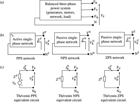
From Figure 2.3(c), sequence voltage and current relations at the point of unbalance F canbe written for each sequence network. For the active PPS network:

     (2.19)

where V_F is the PPS voltage at the point of fault F immediately before the unbalance condition is applied, is the resultant PPS voltage at the point of fault, and is the PPS current flowing out of the PPS network into the point of fault.

For the passive NPS network:

     (2.20)

where is the NPS voltage at the point of fault and is the NPS current flowing out of the NPS network into the point of fault.

For the passive ZPS network:

     (2.21)

where is the ZPS voltage at the point of fault and is the ZPS current flowing out of the ZPS network into the point of fault.

As will be seen in later chapters, the PPS and NPS impedances are the same for most static power system plant but are generally different for rotating machines. In a ZPS network, because ZPS voltages, and ZPS currents, are co-phasal, the ZPS currents can only flow if there is a return connection, through either a neutral or earth wire or the general body of the earth. This is a very important consideration when determining the ZPS equivalent circuits for transformers and the analysis of earth return currents as will be seen in Chapters 4 and 10, respectively.

2.2.5 Sequence components of unbalanced three-phase impedances

Figure 2.4 shows a system of static unbalanced three-phase mutually coupled impedance elements.

Figure 2.4 Unbalanced static mutually coupled three-phase impedances

The voltage drop equations across phases R, Y and B, in matrix form, are given by

(2.22a)

or in concise matrix notation form:

     (2.22b)

where Z_RYB is defined as the phase impedance matrix of the unbalanced three-phase mutually coupled system shown in Figure 2.4. The diagonal elements are the self-impedances of each phase and the off-diagonal elements are the mutual impedances between the phases. It is important to note that this is the impedance matrix in the actual or physical phase frame of reference, RYB, where each impedance is an actual physical element.

What are the PPS, NPS and ZPS impedances of this system and what light do they shed on the use of the symmetrical components’ theory in practice? To answer this question, we substitute Equations (2.11) and (2.15a) into Equation (2.22b), we obtain

and pre-multiplying by H⁻¹, we obtain

     (2.23)

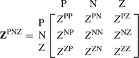
where Z^PNZ is defined as the sequence impedance matrix of the unbalanced three-phase system shown in Figure 2.4 and is given by

     (2.24)

It is important to note that this is the impedance matrix in the sequence frame of reference obtained by transforming the phase impedance matrix according to Equation (2.24) using the transformation matrices shown.

Assuming that the mutual phase impedances are bilateral or reciprocal that is Z_RY = Z_YR, etc., Equation (2.24) becomes

(2.25)

where

     (2.26a)

     (2.26b)

     (2.26c)

     (2.26d)

     (2.26e)

     (2.26f)

Dropping the R notation from the current vector for convenience and using Equations (2.23), (2.24) and (2.25), we can write

     (2.27)

which can be written as

     (2.28)

Equation (2.28) is important and requires a physical explanation. The sequence impedance matrix is full, non-diagonal and non-symmetric. A non-symmetric matrix is exemplified by the different mutual coupling terms b and d (also c and e) in the matrix. A non-diagonal matrix means that mutual coupling between the sequence circuits exist. For example, taking the PPS circuit, the total PPS voltage drop in this circuit consists of three components as follows:

     (2.29)

The first term on the right is the PPS voltage drop induced by the flow of PPS current in the PPS circuit. The second term is an additional PPS voltage drop caused by the flow of NPS current in the NPS circuit acting on the mutual impedance from the PPS to the NPS circuit. The third term is an additional PPS voltage drop caused by the flow of ZPS current in the ZPS circuit acting on the mutual impedance from the PPS to the ZPS circuit.

We have calculated the sequence impedance matrix of a general three-phase mutually coupled system and this turns out to be non-diagonal and non-symmetric. What does this mean in practice? Let us remember that the basic principle of the symmetrical component theory rests on the fact that the PPS, NPS and ZPS sequence circuits are separate with no mutual coupling between them. In mathematical terms, this means that the sequence impedance matrix has to be diagonal so that a PPS voltage drop is produced by the flow of PPS current only, and likewise for the NPS and ZPS circuits. The transformation of the phase impedance matrix of Equation (2.22a) from the phase frame of reference to the sequence frame of reference, Equation (2.28), produced no advantages whatsoever. In such situations, the symmetrical component theory may not be used and analysis in the phase frame of reference is more advantageous.

2.2.6 Sequence components of balanced three-phase impedances

The application of the symmetrical component theory in practical power system short-circuit analysis requires the PPS, NPS and ZPS circuits to be separate and uncoupled. This is achieved by the removal of the off-diagonal mutual elements in the sequence impedance matrix of Equation (2.28) so that the matrix becomes diagonal. This can be accomplished if the physical phase impedances of the original three-phase system shown in Figure 2.4 are assumed to be balanced, i.e. the self-impedances are assumed to be equal, and the mutual impedances are also assumed to be equal, i.e.

     (2.30a)

     (2.30b)

Substituting Equation (2.30) into Equations (2.26) and (2.27), we obtain

     (2.31)

where,

     (2.32a)

     (2.32b)

Also, if the PPS, NPS and ZPS impedances are known, the balanced self and mutual phase impedances can be calculated as follows:

     (2.33a)

     (2.33b)

2.2.7 Advantages of symmetrical components frame of reference

The significant advantage of the symmetrical component theory is that it provides a mathematical method that allows us to decompose the original complex mutually coupled three-phase system equations into three separate sets of equations. The PPS, NPS and ZPS sets of currents and voltages are each calculated from the PPS, NPS and ZPS circuits, respectively, i.e. in the sequence frame of reference. The sequence of currents and voltages are then easily transformed back into the phase frame of reference. However, the creation of three uncoupled single-phase sequence circuits is based on the assumption that the original three-phase system is perfectly balanced. In reality, this is not the case, as will be seen in later chapters. Nonetheless, reasonable assumptions of balance can be made to allow the use of the symmetrical component theory in practical applications. Nowadays, almost all large-scale short-circuit analysis in practical power systems is carried out in the sequence frame of reference with transformation to the phase frame of reference carried out as a final step in the analysis. There are, nonetheless, specialised short-circuit applications where analysis in the phase frame of reference is used. This is discussed in Chapter 6.

2.2.8 Examples

2.3.1 General

In general, there are three types of faults in three-phase power systems. These are short-circuit faults between one or more phases which may or may not involve earth, open-circuit faults on one or two phases and simultaneous faults where more than one fault occurs at the same time at the same or at different locations in the network. Short-circuit faults are sometimes referred to as shunt faults whereas open-circuit faults as series faults. When a short-circuit fault occurs at a point F on the three-phase network, the conditions imposed by the fault at F must be observed between the relevant phase(s) and the neutral point in the sequence networks. However, when an open-circuit fault occurs at a point F in the network, the conditions imposed by the fault must be observed between the two sides of the open circuit, say points F and F′, in the sequence networks. In this section, we will derive methods of connecting the three PPS, NPS and ZPS networks for various fault types that can occur in power systems. The unbalanced fault condition applied in the three-phase network is arranged to be symmetrical with respect to phase R which is taken as the reference phase. This results in simpler mathematical derivation as will be shown later.

2.3.2 Balanced three-phase to earth short-circuit faults

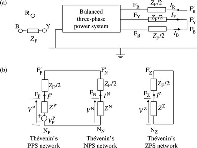
A three-phase to earth short-circuit fault at a point in a three-phase system is a balanced or symmetrical fault that can still be analysed using the symmetrical components theory. Figure 2.5(a) shows the representation of this fault. F_R, F_Y and F_B are points in the three-phase system where the three-phase fault is assumed to occur through the balanced fault impedances Z_F, and F′_R, F′_Y and F′_B are the true points of fault.

Figure 2.5 Balanced three-phase to earth short-circuit fault through a fault impedance Z_F

From Figure 2.5(a), the voltages at point F are given by

     (2.34)

Using Equations (2.6), (2.14a) and (2.19), it can be shown that the sequence voltages and currents at the fault point are given by

     (2.35)

and

     (2.36)

Therefore, the three-phase power system remains balanced and symmetrical after the occurrence of such a fault because the fault impedances are equal in the three phases. Therefore, only PPS voltages exist and only PPS currents can flow.

Since phase R is used as the reference, it is convenient from now on to drop the R notation in the PPS, NPS and ZPS voltage and current equations whilst always remembering that these sequence quantities are those of phase R.

Using Equations (2.15a) and (2.10b), the phase fault currents are given by

     (2.37a)

     (2.37b)

     (2.37c)

and, using Equation (2.34), the phase fault voltages at the fault point F are given by

     (2.38a)

     (2.38b)

     (2.38c)

As expected for a balanced and symmetrical short-circuit fault, the sum of the three-phase currents I_R + I_Y + I_B is equal to zero hence the net fault current flowing into earth is zero. Similarly, the sum of the three-phase voltages V_R + V_Y + V_B is equal to zero. Figure 2.5(b) shows the connections of the Thévenin’s PPS, NPS and ZPS equivalent circuits that satisfy Equations (2.35) and (2.36).

The case of a solid or bolted three-phase to earth short-circuit fault is obtained by setting Z_F = 0.

2.3.3 Balanced three-phase clear of earth short-circuit faults

A three-phase short-circuit fault clear of earth at a point F in a three-phase system is represented by connecting an equal fault impedance between each pair of phases as shown in Figure 2.6(a), i.e., as a delta connection.

Figure 2.6 Balanced three-phase short-circuit fault clear of earth through a fault impedance Z_F

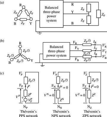
In order to calculate the equivalent fault impedance ‘seen’ in each phase, a transformation of delta to star with isolated neutral is needed as follows:

     (2.39)

The fault representation is illustrated in Figure 2.6(b).

The phase fault currents and voltages are given by

     (2.40a)

and

     (2.40b)

and

     (2.40c)

Using Equations (2.14), (2.19), (2.20) and (2.21), we obtain

     (2.41a)

     (2.41b)

The phase fault currents are given by

     (2.42a)

     (2.42b)

     (2.42c)

The phase fault voltages at point F are given by

     (2.43a)

     (2.43b)

     (2.43c)

Figure 2.6(c) shows the connections of the PPS, NPS and ZPS equivalent networks that satisfy the fault condition at the fault point F. The case of a solid or bolted three-phase clear of earth short-circuit fault is obtained by setting Z_F = 0.

2.3.4 Unbalanced one-phase to earth short-circuit faults

Figure 2.7(a) shows a representation of an unbalanced one-phase to earth fault on phase R through a fault impedance Z_F.

Figure 2.7 Unbalanced one-phase to earth short-circuit fault through a fault impedance Z_F

For ease of notation in the rest of this chapter, we will replace with V_F. The conditions at the point of fault are

     (2.44a)

and

     (2.44b)

Using Equation (2.14) for currents instead of voltages, we obtain

     (2.45)

Substituting Equations (2.19), (2.20) and (2.21) into Equation (2.9a) and using Equation (2.45), we obtain

or

     (2.46)

Thus, the sequence fault currents are given by

     (2.47)

Equations (2.45) and (2.46) show that the PPS, NPS and ZPS networks should be connected in series as shown in Figure 2.7(b) with the fault impedance Z_F appearing as an external impedance in series with each sequence network.

The PPS, NPS and ZPS voltages at the fault point are calculated using Figure 2.7(b) or (c) giving

     (2.48)

     (2.49)

     (2.50)

The phase fault current is calculated using Equations (2.45) and (2.47) giving

     (2.51)

The phase fault voltage is calculated from Equation (2.44) giving

     (2.52)

The phase voltages on the healthy or unfaulted phases at the point of fault can be calculated using Equation (2.9) and Equations (2.48), (2.49) and (2.50) giving

     (2.53)

where

     (2.54)

and

     (2.55)

where

     (2.56)

K_E1 and K_E2 are termed the earth fault factors and have a magnitude that typically range from 1 to 1.8 depending on the method of system earthing used. This factor is the ratio of the rms phase to earth voltage at the fault point during the fault to the rms phase to earth voltage without a fault. This factor determines the extent of voltage rise on the healthy phases during the fault. Systems that are defined as ‘effectively earthed’ are those where the earth fault factor is less than or equal to 1.4.

The case of a solid or bolted single-phase to earth short-circuit fault is obtained by setting Z_F = 0.

2.3.5 Unbalanced phase-to-phase or two-phase short-circuit faults

Figure 2.8(a) shows a representation of an unbalanced two-phase fault on phases Y and B through a fault impedance Z_F.

Figure 2.8 Unbalanced two-phase short-circuit fault through a fault impedance Z_F

The conditions at the point of fault are

     (2.57a)

Substituting the above phase currents into Equation (2.15b), we obtain

     (2.57b)

Substituting I^Z = 0 into Equation (2.21) gives V^Z = 0 and using Equations (2.7) and (2.8), we can write

     (2.58a)

Also, using Equations (2.7b) and (2.8) for phase currents, we obtain

     (2.58b)

Equating V_Y − V_B from Equations (2.57a) and (2.58a), using Equation (2.58b) and I^P = −I^N, we obtain

     (2.59a)

Substituting Equations (2.19) and (2.20) into Equation (2.59a), and using I^P = −I^N, we obtain

     (2.59b)

The sequence fault currents are calculated from Equation (2.59b) using I^P = −I^N giving

     (2.60)

Equations (2.57b) and (2.59b) show that the PPS and NPS networks should be connected in parallel as shown in Figure 2.8(b) with half the fault impedance, 1/2Z_F, appearing as an external impedance in series with the PPS and NPS networks. The ZPS currents and voltages are zero.

The phase fault currents are calculated using Equation (2.15a) giving

     (2.61)

The phase voltages on the faulted phases Y and B are calculated using Equations (2.9b), (2.9c), (2.19), (2.20), (2.21) and (2.60) giving

     (2.62a)

     (2.62b)

The phase voltage on the healthy or unfaulted phase R can be calculated using Equation (2.9a) giving

     (2.63)

The case of a solid or bolted two-phase short-circuit fault is obtained by setting Z_F = 0.

2.3.6 Unbalanced two-phase to earth short-circuit faults

Figure 2.9(a) shows a representation of an unbalanced two-phase to earth fault on phases Y and B through a fault impedance Z_F.

Figure 2.9 Unbalanced two-phase to earth short-circuit fault through a fault impedance Z_F

The conditions at the point of fault are given by

     (2.64)

From Equation (2.7a) for currents, and I_R = 0, we obtain

     (2.65)

Rewriting Equations (2.9b) and (2.9c), and using Equation (2.64), we have

     (2.66a)

     (2.66b)

Subtracting Equation (2.66b) from Equation (2.66a), we obtain

which, using , reduces to

     (2.67)

Now, substituting Equations (2.19) and (2.20) into Equation (2.67), we obtain

     (2.68)

Adding Equations (2.66a) and (2.66b), we obtain

which, using h² +h = -1 and Equations (2.20), (2.21) and (2.67), reduces to

     (2.69a)

and

     (2.69b)

Equations (2.65) and (2.69) show that the PPS, NPS and ZPS networks should be connected in parallel, as shown in Figure 2.9(b), with the fault impedance Z_F appearing as an external impedance in each sequence network.

The sequence fault currents are calculated using Equations (2.65) and (2.69), or alternatively from Figure 2.9(b). The use of the equations is illustrated for deriving the sequence currents. Using Equation (2.69) and expressing I^N and I^Z in terms of I^P then substituting into Equation (2.65), we obtain

which after a little algebra gives

     (2.70a)

     (2.70b)

and

     (2.70c)

The phase fault currents are calculated from the sequence currents using Equation (2.15a) giving

     (2.71a)

and

     (2.71b)

The total fault current flowing into earth at the point of fault is the sum of the phase fault currents I_Y and I_B giving

     (2.72)

The phase voltage on the healthy or unfaulted phase R can be calculated using Equation (2.9a) giving

     (2.73)

The phase voltages on the faulted phases Y and B can be calculated using Equation (2.64) giving

     (2.74a)

     (2.74b)

The case of a solid or bolted two-phase to earth short-circuit fault is obtained by setting Z_F = 0. Also, in the case where an earth impedance Z_E is present in the common connection to earth, as shown in Figure 2.9(c), it can be shown that Z^Z in Figure 2.9(b) must be replaced by (Z^Z + 3Z_E). The reader is encouraged to prove this statement.

2.3.7 Unbalanced one-phase open-circuit faults

Figure 2.10(a) shows the representation of an unbalanced one-phase open-circuit fault occurring on phase R and creating points F and F′ in a balanced three-phase power system.

Figure 2.10 Unbalanced one-phase open-circuit fault

The conditions imposed by the fault are

     (2.75)

Equation (2.75) represents the sequence currents of the phase current I_R from points F to F′. In addition, since these two points are still connected together on phases Y and B, we have

     (2.76)

The sequence components of the voltages in Equation (2.76) can be calculated using Equation (2.14) giving

     (2.77)

Equations (2.75) and (2.77) are satisfied by connecting the PPS, NPS and ZPS equivalent networks in parallel at points F to F′ as shown in Figure 2.10(b). It should be noted that Z^P, Z^N, and Z^Z are the PPS, NPS and ZPS equivalent Thévenin impedances, respectively, as ‘seen’ looking back into the respective sequence network from between the points F and F′. The voltage source in the PPS equivalent network in Figure 2.10(b) has not been derived yet. This voltage source is the open-circuit PPS voltage appearing across F and F′. This voltage is calculated as the multiplication of the prefault load current in phase R, i.e. the current flowing before the open circuit occurs (note that this is a PPS current because the three-phase power system is balanced), and Z^P, i.e.

     (2.78)

From Figure 2.10(b), the PPS current is given by

     (2.79)

The NPS current is given by

or

     (2.80)

The ZPS current is given by

or

     (2.81)

The sequence voltages are given by

     (2.82)

and the phase voltage across the open circuit is given by

     (2.83)

2.3.8 Unbalanced two-phase open-circuit faults

Figure 2.11(a) shows a representation of an unbalanced two-phase open-circuit fault occurring on phases Y and B and creating points F and F′ in a balanced three-phase power system.

Figure 2.11 Unbalanced two-phase open-circuit fault

The conditions imposed by the fault are given by

     (2.84a)

The sequence current components in Equation (2.84a) are given by

     (2.84b)

In addition, since points F to F′ are still connected together on phase R

     (2.85)

Equations (2.84b) and (2.85) are satisfied by connecting the PPS, NPS and ZPS equivalent networks in series at the points F to F′ as shown in Figure 2.11(b). From this, the sequence currents are given by

     (2.86)

where I_L is the prefault current flowing in phase R between F and F′ just before the open-circuit fault occurs on phases Y and B.

The sequence voltages are given by

     (2.87a)

     (2.87b)

     (2.87c)

The phase voltages on the faulted phases Y and B are calculated using Equations (2.9b) and (2.9c) giving

     (2.88a)

     (2.88b)

The case of a three-phase open-circuit fault does not require any consideration since this is not normally a fault but rather a normal switching operation in power systems such as the opening of the three phases of a circuit-breaker. Only PPS currents and voltages continue to exist in the resulting balanced power system. Such studies that involve the opening of the three phases of circuit-breakers, for example, to simulate the disconnection of a circuit and calculate the resultant currents, voltages active and reactive power flows, are known as PPS power flow studies.

2.3.9 Example

2.4.1 General

The mathematical equations derived in previous sections for unbalanced short-circuit and open-circuit faults were based on arranging the unbalance conditions to be symmetrical about phase R which was taken as the reference phase. In this section, we will show that whilst any phase could be chosen as the reference, the choice of phase R results in the simplest mathematical derivations.

2.4.2 One-phase to earth short-circuit faults

In the case of a one-phase to earth short circuit on phase R with phase R chosen as the reference, the symmetrical components of the faulted phase are given by

     (2.89)

The above equations are represented in Figure 2.7.

However, for a one-phase to earth short circuit on phase Y with phase Y chosen as the reference, the symmetrical components of the faulted phase are given by

     (2.90)

Expressing the sequence currents and voltages of Equation (2.90) in terms of phase R using Equation (2.8), we obtain

     (2.91)

Similarly, for a one-phase to earth short circuit on phase B with phase B chosen as the reference, the symmetrical components of the faulted phase are given by

     (2.92)

Expressing the sequence currents and voltages of Equation (2.92) in terms of phase R using Equation (2.8), we obtain

     (2.93)

Equations (2.89), (2.91) and (2.93) can be represented by the connection of the PPS, NPS and ZPS networks as shown in Figure 2.12. The sequence networks are still connected in series but through three complex multipliers k^P, k^N and k^Z. These multipliers are applied to the sequence voltages and currents and are equal to either 1, h or h² according to Equations (2.89), (2.91) and (2.93) and as shown in Case 1 in Figure 2.12. The function of the multiplier is to apply the same phase shift to the relevant sequence current and voltage whilst keeping their magnitudes unchanged. In describing this multiplier, we have deliberately avoided the use of the term phase shifting transformer so as to avoid confusion with the property of physical transformers that transform voltages and currents by inverse ratios or multipliers.

Figure 2.12 One-phase short-circuit fault on either phase R, Y or B

Figure 2.12 shows that the phase shifts are applied to the PPS and NPS voltages and currents for faults on either phase Y or B. However, the ZPS current and voltage multiplier is always equal to unity.

For convenience in practical analysis, it is normal to avoid applying phase shifts to the active PPS network, which contains generating or voltage sources, and instead apply the phase shifts to the passive NPS and ZPS networks. This is easily accomplished by dividing Equations (2.91) and (2.93) by h² and h, respectively, and the resulting multipliers k^P, k^N and k^Z are as shown in Case 2 in Figure 2.12.

In summary, in the case of a single-phase to earth short-circuit fault on any phase in a three-phase network, the assumption of the fault being on phase R results in the simplest mathematical equations because the three multipliers k^P, k^N and k^Z are all equal to unity.

2.4.3 Two-phase to earth short-circuit faults

For a two-phase to earth short-circuit fault, we have three cases as follows:

or expressed in terms of phase R

     (2.96b)

Equations (2.94), (2.95b) and (2.7b) can be represented by the connection of the PPS, NPS and ZPS networks as shown in Figure 2.13. The sequence networks are still connected in parallel but through three complex multipliers k^P, k^N and k^Z that are equal to either 1, h or h² according to Equations (2.95b) and (2.96b) as shown in Case 1 in Figure 2.13. Again, applying phase shifts to the active PPS network can be avoided by dividing Equations (2.95b) and (2.96b) by h² and h, respectively, and the resulting multipliers k^P, k^N and k^Z are as shown in Case 2 in Figure 2.13.

Figure 2.13 Two-phase to earth short circuit on Y−B−E, R−B−E or R−Y−E

A comparison of the tables showing the complex multipliers k^P, k^N and k^Z in Figures 2.12 and 2.13 show that for the same reference phase, each multiplier, k^P, k^N or k^Z, has the same value irrespective of the fault type.

The methodology presented can be easily extended to any other unbalanced short-circuit or unbalanced open-circuit fault. The reader is encouraged to repeat the analysis for other fault conditions. These include: (a) a one-phase open-circuit fault on any phase, i.e. R or Y or B; (b) a two-phase open-circuit fault on any two phases, i.e. R-Y or Y-B or R-B; and (c) a two-phase short-circuit fault on any two phases, i.e. R-Y or Y-B or R-B.

2.5.1 General

Simultaneous faults are more than one fault that occur at the same time in a three-phase power system either at the same or at different locations. Because there is a very large theoretical combination of such faults, we will limit our attention to a representative number of cases that are of practical interest. These are three cases of two simultaneous faults and one case of three simultaneous faults. The analysis of simultaneous faults can be simplified by deriving the conditions at the fault locations with respect to the same reference phase, i.e. phase R. These conditions determine the method of connection of the PPS, NPS and ZPS networks. In this analysis, we assume that the full network has been reduced to an equivalent as seen from the faulted boundary locations and the latter, denoted as nodes J and L, have been retained. Network reduction is discussed in detail in Chapter 8.

2.5.2 Simultaneous short-circuit faults at the same location

The two-simultaneous faults we consider are illustrated in Figure 2.14(a) and consist of a solid one-phase to earth short-circuit fault and a solid two-phase short-circuit fault. Conceptually, since all three phases are faulted, the two faults can also be considered as a single three-phase unbalanced fault! Using phase R as the reference phase, the single-phase short circuit assumed to occur on phase R and the two-phase short circuit assumed to occur on phases Y and B, the conditions at the fault location are given by

Figure 2.14 Simultaneous one-phase to earth and two-phase short-circuits at the same location, or three-phase unbalanced short-circuit fault

     (2.97)

Using Equations (2.9b) and (2.9c) for I_Y and I_B instead of voltages, we obtain

     (2.98)

Substituting Equations (2.19), (2.20) and (2.21) for PPS, NPS and ZPS voltages at the fault point into Equations (2.9), we have

     (2.99a)

     (2.99b)

and

     (2.99c)

Adding Equations (2.99), we obtain V_R + V_Y + V_B = −3Z^ZI^Z = 2V_Y = 2V_B or

     (2.100)

Also, using Equations (2.99b) and (2.99c) as well as V_Y = V_B from Equation (2.97), we have V_Y − hV_B = (1 − h)V_Y = (1 − h)(Z^NI^N − Z^ZI^Z) or

     (2.101)

Equating Equations (2.100) and (2.101), we obtain

     (2.102)

Substituting Equation (2.102) into Equation (2.98), we obtain

     (2.103)

Substituting Equations (2.103) into Equation (2.99a), the sequence fault currents are

     (2.104a)

     (2.104b)

     (2.104c)

Using Equation (2.9), the phase fault currents are given by

     (2.105a)

     (2.105b)

Subtracting Equation (2.9c) from Equation (2.9b) and using V_Y = V_B, we obtain V^P = V^N. Using Equation (2.9a) with V_R = 0 and V^P = V^N, we obtain V^Z = -2V^P. Using Equation (2.20), we obtain

     (2.106a)

and

     (2.106b)

Finally, using Equation (2.100), the phase voltages on phases Y and B are given by

     (2.106c)

Using Equation (2.98) or I^Z = (I^P + I^N)/2 and V^Z = −2V^P = −2V^N, the equivalent circuit of this simultaneous fault condition is shown in Figure 2.14(b).

It should be noted that the real transformation ratio acts on voltage and current as a normal ideal transformer does.

2.5.3 Cross-country faults or simultaneous faults at different locations

A cross-country fault is a condition where there are two simultaneous one-phase to earth short-circuit faults affecting the same circuit but at different locations and possibly involving different phases. Therefore, the fault conditions are a one-phase to earth, phase R-Earth (E) short-circuit fault at location J and one-phase to earth short-circuit fault on either R-E, Y-E or B-E at location L. The fault conditions at both fault locations are given as follows:

Location J: R-E short-circuit fault

     (2.107)

Location L: R-E short-circuit fault

     (2.108)

Location L: Y-E short-circuit fault

or

     (2.109)

Location L: B-E short-circuit fault

or

     (2.110)

Figure 2.15 shows the connection of the PPS, NPS and ZPS networks at the two fault locations J and L using the three sets of Equations (2.107) and (2.108), (2.107) and (2.109), and (2.107) and (2.110).

Figure 2.15 Cross-country simultaneous one-phase to earth short-circuit faults

Straightforward analysis using Kirchoff’s voltage and current laws can be carried out using Figure 2.15.

2.5.4 Simultaneous open-circuit and short-circuit faults at the same location

We now consider a one-phase open-circuit fault on phase R at location J and a one-phase to earth short-circuit fault R-E or Y-E or B-E at the same location.

The conditions created by the open-circuit fault on phase R at location J creating open-circuit J-J′ are given by

     (2.111)

The conditions created by a R-E short-circuit fault at location J are given by

     (2.112)

The conditions created by a Y-E short-circuit fault at location J are given by

or

     (2.113)

The conditions created by a B-E short-circuit fault at location J are given by

or

     (2.114)

Figure 2.16 shows the connection of the PPS, NPS and ZPS networks using the three sets of Equations (2.111) and (2.112), (2.111) and (2.113), and (2.111) and (2.114).

Figure 2.16 Simultaneous one-phase open-circuit and one-phase short-circuit faults

Straightforward analysis using Kirchoff’s voltage and current laws can be carried out using Figure 2.16.

2.5.5 Simultaneous faults caused by broken and fallen to earth conductors

Figure 2.17 illustrates a one-phase open-circuit fault on phase R caused by a broken phase conductor. The conductors on both sides of the open circuit are assumed to fall to earth thus creating a one-phase to earth short-circuit fault on each side.

Figure 2.17 Three simultaneous faults caused by a broken and fallen to earth conductor

The conditions created by the open-circuit fault on phase R creating open-circuit J-J′ are given by

     (2.115)

Short-circuit fault on phase R at location J

     (2.116)

Short-circuit fault on phase R at location J′

     (2.117)

Figure 2.17 shows the connection of the PPS, NPS and ZPS networks using Equations (2.115), (2.116) and (2.117).

Straightforward analysis using Kirchoff’s voltage and current laws can be carried out using Figure 2.17.

2.5.6 Simultaneous short-circuit and open-circuit faults on distribution transformers

We will now analyse in detail a simultaneous fault case that involves a two-winding distribution transformer that is extensively used in distribution substations. The high voltage winding is delta connected with fuses being used as incoming protection against high currents. The low voltage winding is star connected with the neutral solidly earthed and the transformer supplies a balanced three-phase load. The simultaneous faults may be created when a short-circuit fault occurs on the transformer low voltage side which causes one fuse to blow and clear before the other fuses, or a circuit-breaker upstream, open and clear the fault. This can lead to a situation where the short-circuit currents are too low to operate any further protection so that the prolonged duration of such currents may overstress or even damage power plant. The transformer is assumed to supply a balanced star-connected three-phase static load having an impedance per phase of Z_L and therefore the corresponding load PPS, NPS and ZPS impedances are all equal to Z_L. The detailed sequence modelling of transformers will be covered in Chapter 4, but we will present this case now because of its practical importance and relevance in this chapter. We will also make use of the transformer phase shifts introduced by the star-delta winding connections and presented in Chapter 4, and we will consider the transformer vector group to be D11yn or in accordance with American ANSI standard. This means that when stepping up from the low voltage to the high voltage side, the transformer’s PPS currents (and voltages) are advanced by 30° whereas the NPS currents (and voltages) are retarded by 30°. The simultaneous faults are illustrated in Figure 2.18(a) and the equivalent sequence network connections are shown in Figure 2.18(b).

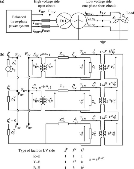
Figure 2.18 Simultaneous one-phase short circuit on transformer low voltage side and one-phase open circuit on transformer high voltage side

From Figure 2.18(b), the following relations can be written

     (2.118)

     (2.119)

     (2.120)

     (2.121)

Therefore, from the above current equations, we obtain

     (2.122)

and

     (2.123)

Applying Kirchoff’s voltage law to the high voltage side of the PPS network of Figure 2.18(b), we obtain or using Equations (2.118)-(2.121)

     (2.124)

Applying Kirchoff’s voltage law to the low voltage side of the PPS network of Figure 2.18(b), and after a little algebra, we obtain

     (2.125)

Applying Kirchoff’s voltage law to the low voltage side of the NPS network of Figure 2.18(b), and using Equation (2.122), we obtain

     (2.126)

Substituting Equations (2.125) and (2.126) into Equation (2.124), and using Equation (2.123), we obtain, after a little algebra

     (2.127)

Using Equations (2.122) and (2.123) as well as Figure 2.18(b), the PPS, NPS and ZPS voltages at the short-circuit fault point are given by

     (2.128)

     (2.129)

From the low voltage side of the ZPS network of Figure 2.18(b), we have which, using Equation (2.123) and Figure 2.18(b) becomes

     (2.130)

Now, by substituting Equations (2.128), (2.129) and (2.130) into the sequence voltages of Equation (2.121), we can express I^N_F in terms of I^P_LV as

     (2.131)

Substituting Equation (2.131) into Equation (2.127) and solving for I^P_LV, we obtain

     (2.132)

The calculation of I^P_LV enables us to calculate the required sequence currents and voltages in Figure (2.18b) using Equations (2.118) to (2.131) by back substitution. We will present in Chapter 6 that the voltage source V_S is calculated from the initial load flow solution just before the occurrence of the short-circuit fault as follows:

     (2.133)

The short-circuit fault current on the faulted phase can be calculated from Equation (2.123) as follows:

     (2.134)

The corresponding currents on the high voltage side can be calculated using Equations (2.15a), (2.118), (2.119) and (2.122) to give

     (2.135)

and

     (2.136)

The reader is encouraged to repeat the above analysis for a solid two-phase to earth short-circuit fault on the transformer low voltage side considering all three fault combinations of R−Y−E, R−B−E and Y−B−E.